Multipole approach for photo- and electroproduction of kaon

Abstract

We have analyzed the experimental data on $K^{+}\Lambda$ photoproduction by using a multipole approach. In this analysis we use the background amplitudes constructed from appropriate Feynman diagrams in a gauge-invariant and crossing-symmetric fashion. Results of our analysis reveal the problem of mutual consistency between the new SAPHIR and CLAS data. We found that the problem could lead to different conclusions on “missing resonances”. We have also extended our analysis to the finite $Q^{2}$ region and compared the result with the corresponding electroproduction data.

1 Introduction

In the last decades, there have been a large number of attempts devoted to understand hadronic interactions in the medium energy region. However, due to the nonperturbative nature of QCD at these energies, hadronic physics continues to be a challenging field of investigation.

One of the most intensively studied topics in the realm of hadronic physics is the associated strangeness photoproduction. High-intensity continuous electron beams produced by modern accelerator technologies, along with unprecedented precise detectors, are among the important aspects that have brought renewed attention to this subject.

On the other hand, the argument that some of the resonances predicted by constituent quark models are strongly coupled to strangeness channels, and therefore intangible to $\pi N\to\pi N$ reactions that are used by Particle Data Group (PDG) to extract the properties of nucleon resonances, has raised the issue of “missing” resonances. As a consequence, recent analyses of strangeness photoproduction have mostly focused on the quest of missing resonances Mart:1999ed . With the new CLAS data appearing this year Bradford:2005pt , this becomes an arduous task, since several recent phenomenological studies found a lack of mutual consistency between the recent CLAS and SAPHIR Glander:2003jw data.

In view of this, it is certainly important to investigate the physics consequence of using each data set. Ideally, this should be performed on the basis of a coupled-channels formalism. However, the level of complexity in such a framework increases quickly with the addition of resonance states. It is widely known that in kaon photoproduction too many resonance states can contribute, whereas there is a lack of systematic procedure to determine how many resonances should be built into the process. Thus, for this purpose, we constrain the present work to a single-channel analysis, but we use as much as possible nucleon resonances listed by PDG. This has the advantage that we can simultaneously explore the importance of higher spin states in kaon photoproduction.

2 Kaon Photoproduction

2.1 Formalism

The background amplitudes are obtained from a series of tree-level Feynman diagrams. They consist of the standard $s$-, $u$-, and $t$-channel Born terms along with the $K^{*}(892)$ and $K_{1}(1270)$ $t$-channel vector mesons. Altogether they are often called extended Born terms.

The resonant multipoles for a state with the mass $M_{R}$, width $\Gamma$, and angular momentum $\ell$ are assumed to have the Breit-Wigner form Tiator:2003uu

$$A_{\ell\pm}^{R}(W)={\bar{A}}_{\ell\pm}^{R}c_{KY}\frac{f_{\gamma R}(W)\Gamma_{\rm tot}(W)M_{R}\,f_{KR}(W)}{M_{R}^{2}-W^{2}-iM_{R}\Gamma_{\rm tot}(W)}e^{i\phi},~{}$$ (1)

where $W$ represents the total c.m. energy, the isospin factor $c_{KY}$ is $-1$, $f_{KR}$ is the usual Breit-Wigner factor describing the decay of a resonance $R$ with a total width $\Gamma_{\rm tot}(W)$ and physical mass $M_{R}$. The $f_{\gamma R}$ indicates the $\gamma NR$ vertex and $\phi$ represents the phase angle. The Breit-Wigner factor $f_{KR}$ is given by

$$f_{KR}(W) = \left[\frac{1}{(2j+1)\pi}\frac{k_{W}}{|\mbox{\boldmath${q}$}|}\frac{m_{N}}{W}\frac{\Gamma_{KY}}{\Gamma_{\rm tot}^{2}}\right]^{1/2}~{},$$ (2)

with $m_{N}$ and $k_{W}$ indicating the nucleon mass and the photon equivalent energy, respectively. The energy dependent partial width $\Gamma_{KY}$ is defined through

$$\Gamma_{KY} = \beta_{K}\Gamma_{R}\left(\frac{|\mbox{\boldmath${q}$}|}{q_{R}}\right)^{2\ell+1}\,\left(\frac{X^{2}+q_{R}^{2}}{X^{2}+\mbox{\boldmath${q}$}^{2}}\right)^{\ell}\frac{W_{R}}{W}~{},$$ (3)

where the damping parameter $X$ is assumed to be 500 MeV for all resonances, $\beta_{K}$ is the single kaon branching ratio, $\Gamma_{R}$ and $q_{R}$ are the total width and kaon c.m. momentum at $W=M_{R}$. The $\gamma NR$ vertex is parameterized through

$$f_{\gamma R} = \left(\frac{k_{W}}{k_{R}}\right)^{2\ell^{\prime}+1}\,\left(\frac{X^{2}+k_{R}^{2}}{X^{2}+k_{W}^{2}}\right)^{\ell^{\prime}}~{},$$ (4)

where $k_{R}$ is equal to $k_{W}$ calculated at $W=M_{R}$. For $M_{\ell\pm}$ and $E_{\ell+}$: $\ell^{\prime}=\ell$, whereas for $E_{\ell-}$: $\ell^{\prime}=\ell-2$ if $\ell\geq 2$. The values of $\ell$ and $\ell^{\prime}$ as well as other parameters are given in Ref. Mart:2006dk . All observables can be calculated from the CGLN amplitudes

$${\cal F}\! = \!\mbox{\boldmath${\sigma}$}\cdot\mbox{\boldmath${b}$}F_{1}-i\mbox{\boldmath${\sigma}$}\cdot\hat{\mbox{\boldmath${q}$}}~{}\mbox{\boldmath${\sigma}$}\cdot(\hat{\mbox{\boldmath${k}$}}\times\mbox{\boldmath${b}$})F_{2}+\mbox{\boldmath${\sigma}$}\cdot\hat{\mbox{\boldmath${k}$}}~{}\hat{\mbox{\boldmath${q}$}}\cdot\mbox{\boldmath${b}$}F_{3}$$ (5)

$$+\mbox{\boldmath${\sigma}$}\cdot\hat{\mbox{\boldmath${q}$}}~{}\hat{\mbox{\boldmath${q}$}}\cdot\mbox{\boldmath${b}$}F_{4}-\mbox{\boldmath${\sigma}$}\cdot\hat{\mbox{\boldmath${q}$}}~{}b_{0}F_{5}-\mbox{\boldmath${\sigma}$}\cdot\hat{\mbox{\boldmath${k}$}}~{}b_{0}F_{6}$$

where $b_{\mu}=\epsilon_{\mu}-({\hat{\mbox{\boldmath${k}$}}\cdot\mbox{\boldmath${\epsilon}$}}/{|\mbox{\boldmath${k}$}|})k_{\mu}$. For photoproduction only the first four amplitudes $F_{i}$ are relevant. They are related to the electric and magnetic multipoles given in Eq. (1) by

$$F_{1} = \sum_{\ell\geq 0}\left\{\left(\ell M_{\ell+}\!+E_{\ell+}\right)P^{\prime}_{\ell\!+\!1}+\left[\left(\ell+1\right)M_{\ell-}\!+E_{\ell-}\right]P^{\prime}_{\ell-1}\right\}\!,$$

$$F_{2} = \sum_{\ell\geq 1}\left[\left(\ell+1\right)M_{\ell+}+\ell M_{\ell-}\right]P^{\prime}_{\ell},$$

$$F_{3} = \sum_{\ell\geq 1}\left[\left(E_{\ell+}-M_{\ell+}\right)P^{\prime\prime}_{\ell+1}+\left(E_{\ell-}+M_{\ell-}\right)P^{\prime\prime}_{\ell-1}\right],$$

$$F_{4} = \sum_{\ell\geq 2}\left(M_{\ell+}-E_{\ell+}-M_{\ell-}-E_{\ell-}\right)P^{\prime\prime}_{\ell}.$$

2.2 Numerical Results

The number of free parameters is relatively large. To reduce this we fix both $g_{K\Lambda N}$ and $g_{K\Sigma N}$ coupling constants to the SU(3) predictions and fix masses as well as widths of the four-star resonances to their PDG values. Due to the problem of mutual consistency between SAPHIR and CLAS data, in the fitting procedure we define two different data sets. In the first set (Fit 1) we use the SAPHIR and LEPS data, while in the second one (Fit 2) we use the CLAS and LEPS data. In total we use 15 nucleon resonances listed by PDG. The $\chi^{2}$ minimization fit is performed by using the CERN-MINUIT code.

To further investigate the importance of the individual resonances we define a parameter

$$\Delta\chi^{2}~{}=~{}\frac{\chi^{2}_{\rm All}-\chi^{2}_{{\rm All}-N^{*}}}{\chi^{2}_{\rm All}}\times 100\,\%~{},$$ (7)

where $\chi^{2}_{\rm All}$ is the $\chi^{2}$ obtained by using all resonances and $\chi^{2}_{{\rm All}-N^{*}}$ is the $\chi^{2}$ obtained by using all but a specific resonance. Therefore, $\Delta\chi^{2}$ measures the relative difference between the $\chi^{2}$ of including and of excluding the corresponding resonance. The result is shown in the histogram of Fig. 1.

Except for $S_{11}(2090)$, $P_{11}(1710)$, $D_{13}(2080)$, $F_{15}(1680)$, and $G_{19}(2250)$, for which the $\Delta\chi^{2}$ are almost similar, the histogram shows that the new CLAS and SAPHIR data can be only explained by different sets of nucleon resonances. Constraining the $\Delta\chi^{2}\gtrsim 6\%$, e.g., leads to the fact that the important resonances in Fit 1 are the $S_{11}(1650)$, $P_{13}(1720)$, $D_{13}(1700)$, $D_{13}(2080)$, $F_{15}(1680)$, and $F_{15}(2000)$, while Fit 2 needs the $P_{13}(1900)$, $D_{13}(2080)$, $D_{15}(1675)$, $F_{15}(1680)$, and $F_{17}(1990)$.

It is interesting to note here that both Fit 1 and Fit 2 support the requirement of the $D_{13}(2080)$ in this process. Surprisingly, all new data reject the need for the $P_{11}(1710)$, while the new CLAS data do not require the $P_{13}(1720)$ resonance. Although most recent analyses of the $K^{+}\Lambda$ channel have included these intermediate states, this conclusion corroborates the finding of Ref. Arndt:2003ga .

Another new phenomenon is the contribution from the $F_{15}(2000)$ and $F_{17}(1900)$, which are quite important according to SAPHIR and CLAS data, respectively. These resonances have not been used in most analyses, especially in the isobar model with diagrammatic technique, since propagators for spins 5/2 and 7/2 are not only quite complicated in this approach, but also their forms are not unique.

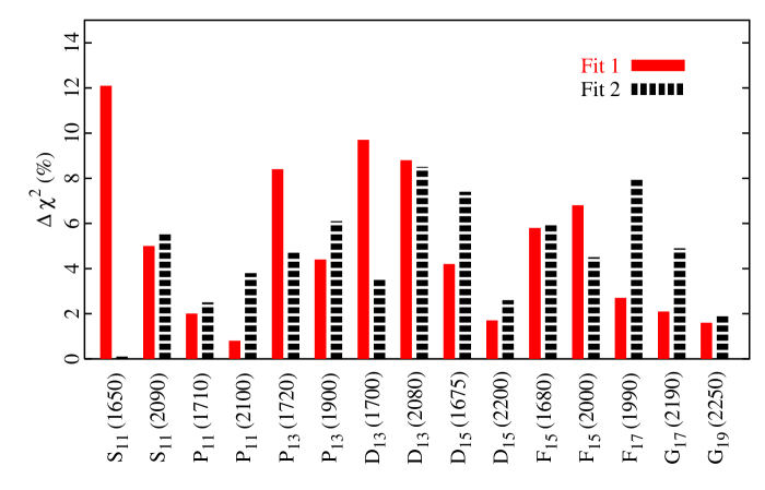
Figure 1: Significance of the individual resonances in our fits.

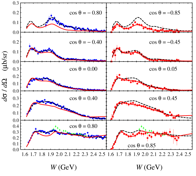
Figure 2: Differential cross sections obtained from Fit 1 (solid curves) and Fit 2 (dashed curves) as a function of the total c.m. energy. Solid circles, squares, and triangles represent experimental data from the CLAS, SAPHIR, and LEPS collaborations, respectively.

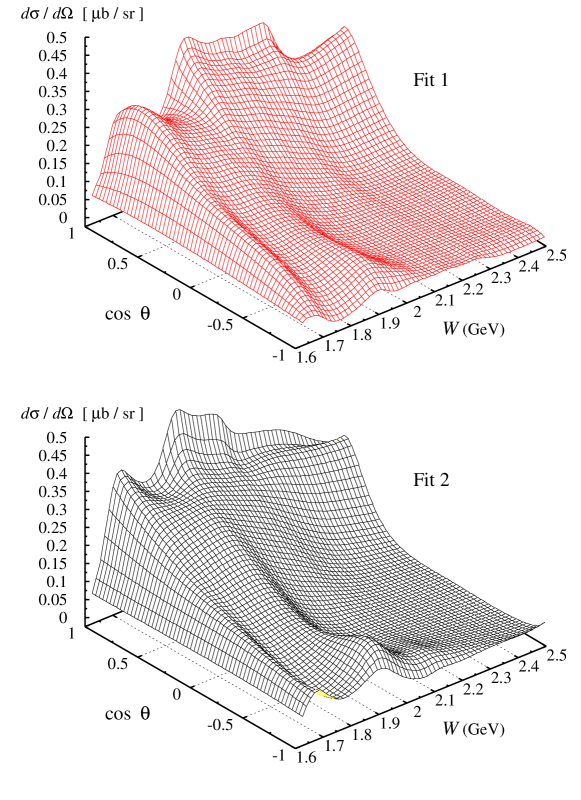
Figure 3: Differential cross sections obtained from Fit 1 and Fit 2 as functions of $W$ and $\cos\theta_{K}$.

In Fig. 2 we show the comparison between the results of Fit 1 and Fit 2 with the CLAS data. The LEPS data are also shown in this case. It is obvious from the figure that the LEPS data are closer to the CLAS data. From this figure it is also clear that the largest discrepancy appears between $W=1.75$ GeV and 1.95 GeV in the forward direction, whereas in the backward direction the discrepancies show up in a wider range, i.e., from 1.8 to 2.4 GeV. It is also important to note that at the very forward and backward angles the two data sets exhibit very different trends. The CLAS data tend to rise at these regions, while the SAPHIR data tend to decrease. Nevertheless, this does not happen in the whole energy region. Especially near the forward angles, where we found that the result of Fit 2 (the new CLAS data) shows more structures than that of Fit 1. To have a better view of this, in Fig. 3 we present the three-dimensional plot of the differential cross section as functions of $W$ and $\cos\theta$.

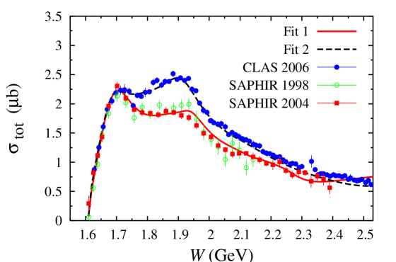
Figure 4: Comparison between experimental total cross sections with the predictions of Fit 1 and Fit 2. Experimental data shown in this figure were not used in the two fits.

Prediction for the total cross sections of both fits is shown in Fig. 4. From this figure it is clear that the extracted total cross sections from both collaborations are consistent with their differential cross sections.

We have investigated the origin of the second peak at $W\approx 1.9$ GeV as shown in Fig. 4. The result indicates that in both fits the peak originates from the $D_{13}(2080)$ with a mass of 1936 MeV if SAPHIR data were used or 1915 MeV if CLAS data were used. This result is in good agreement with the finding from several recent studies Mart:2004ug ; Bartholomy:2004uz ; Julia-Diaz:2006is

3 Kaon Electroproduction

For kaon electroproduction the longitudinal amplitudes $F_{5}$ and $F_{6}$ should be taken into account in Eq. (5). These amplitudes are given by

$$F_{5} = \sum_{\ell\geq 0}\left\{(\ell+1)L_{\ell+}P^{\prime}_{\ell+1}-\ell L_{\ell-}P^{\prime}_{\ell-1}\right\},$$ (8)

$$F_{6} = \sum_{\ell\geq 1}\left\{\ell L_{\ell-}-(\ell+1)L_{\ell+}\right\}P^{\prime}_{\ell},$$ (9)

where the longitudinal multipoles are related to the scalar ones by $L_{\ell\pm}=k_{0}S_{\ell\pm}/|\mbox{\boldmath${k}$}|$.

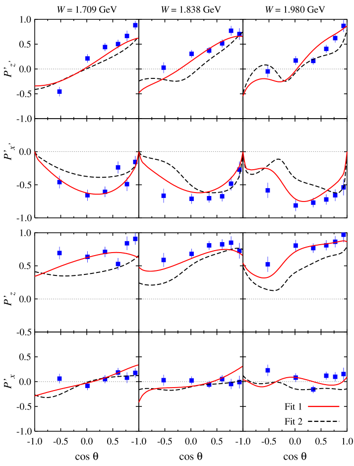
Figure 5: Transfered $\Lambda$ polarization components $P^{\prime}_{z^{\prime}}$ and $P^{\prime}_{x^{\prime}}$ (upper panels) and $P^{\prime}_{z}$ and $P^{\prime}_{x}$ (lower panels) obtained from the two models compared with the new CLAS measurement Carman:2002se . Here, both $Q^{2}$ and $\Phi_{K}$ have been averaged.

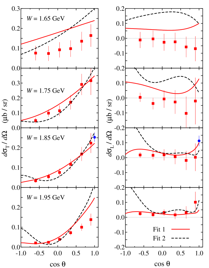
Figure 6: Comparison between the calculated longitudinal and transverse differential cross sections with the new CLAS data Ambrozewicz at $Q^{2}=1$ GeV. Except the two data points shown by solid circles at $W=1.85$ GeV Mohring:2002tr , all data are not used in the fits.

For the nucleon we use the standard Dirac and Pauli form factors, whereas for the kaon we adopt the vector-meson-dominance model. The dependence of the ${\bar{A}}_{\ell\pm}^{R}$ multipole to the $Q^{2}$ is assumed to be

$${\bar{A}}_{\ell\pm}^{R}(Q^{2}) = {\bar{A}}_{\ell\pm}^{R}(0)\,(1+a_{1}Q^{2})\,e^{-a_{2}Q^{2}}~{},$$ (10)

where $a_{1}$ and $a_{2}$ are fitting parameters.

In the fitting database we used 178 data points, including the transfered $\Lambda$ polarization components $P^{\prime}_{z^{\prime}}$, $P^{\prime}_{x^{\prime}}$, $P^{\prime}_{z}$ and $P^{\prime}_{x}$ data from CLAS Carman:2002se . Note that in the latter we do not use the data which are averaged over $Q^{2}$ and $d\Omega$ due to their accuracies and, furthermore, it is found that they are relatively difficult to fit. The comparison between experimental data and our calculation for the transfered $\Lambda$ polarization components is shown in Fig. 5. Surprisingly, Fit 1 (obtained from fitting to the SAPHIR photoproduction data) yields a better explanation of the CLAS transfered $\Lambda$ polarization data.

Very recently, the CLAS collaboration has completed its analysis and published a relatively large number of kaon electroproduction data Ambrozewicz . These data are also not used in the fit, for practical reasons, but we compare them with the result of the present analysis in Fig. 6. As can be seen from this figure, the same conclusion (as for the transfered $\Lambda$ polarization) can be drawn from this result.

4 Conclusion

We have analyzed the $K\Lambda$ photo- and electroproduction data by using a multipole approach and the latest available experimental data. Our results show that the discrepancy between CLAS and SAPHIR photoproduction data results in substantially different calculated electroproduction observables. Surprisingly, the new CLAS electroproduction measurements can be better explained by a model that fits the SAPHIR data. Our next goal is to consider the $K\Sigma$ channels. These channels are of interest because they can be related by using isospin symmetry Mart:1995wu .

References

- (1) T. Mart and C. Bennhold, Phys. Rev. C 61 (1999) 012201.
- (2) R. Bradford et al., Phys. Rev. C 73 (2006) 035202.
- (3) K. H. Glander et al., Eur. Phys. J. A 19 (2004) 251.
- (4) L. Tiator et al., Eur. Phys. J. A 19 (2004) 55.
- (5) T. Mart and A. Sulaksono, Phys. Rev. C 74 (2006) 055203.
- (6) R. A. Arndt et al., Phys. Rev. C 69 (2004) 035208.
- (7) T. Mart, A. Sulaksono and C. Bennhold, nucl-th/0411035.
- (8) O. Bartholomy et al., Phys. Rev. Lett. 94 (2005) 012003.
- (9) B. Julia-Diaz, B. Saghai, T.S. Lee and F. Tabakin, Phys. Rev. C 73 (2006) 055204.
- (10) R. M. Mohring et al., Phys. Rev. C 67 (2003) 055205.
- (11) D. S. Carman et al., Phys. Rev. Lett. 90 (2003) 131804.
- (12) P. Ambrozewicz et al., hep-ex/0611036.
- (13) T. Mart, C. Bennhold and C. E. Hyde-Wright, Phys. Rev. C 51 (1995) R1074.