Gauge-Invariant Formulation of Adiabatic Self-Consistent Collective Coordinate Method

Abstract

The adiabatic self-consistent collective coordinate (ASCC) method is a practical microscopic theory of large-amplitude collective motions in nuclei with superfluidity. We show that its basic equations are invariant against transformations involving the gauge angle in the particle-number space. By virtue of this invariance, a clean separation between the large-amplitude collective motion and the pairing rotational motion can be achieved, enabling us to restore the particle-number symmetry broken by the Hartree-Fock-Bogoliubov (HFB) approximation. We formulate the ASCC method explicitly in a gauge-invariant form. In solving the ASCC equations, it is necessary to fix the gauge. Applying this new formulation to the multi-$O$(4) model, we compare different gauge-fixing procedures and demonstrate that calculations using different gauges indeed yield the same results for gauge-invariant quantities, such as the collective path and quantum spectra. We suggest a gauge-fixing prescription that seems most convenient in realistic calculations.

1 Introduction

Construction of the microscopic theory of large amplitude collective motion is a long-standing and fundamental subject of nuclear many-body problem. [1, 2, 3, 4, 5, 6, 7, 8, 9, 10, 11, 12, 13, 14, 15, 16, 17, 18, 19, 20, 21, 22, 23, 24, 25, 26, 27, 28, 29, 30, 31, 32, 33, 34, 35]. As is well known, pairing correlations play crucial roles in low-lying states of medium and heavy mass nuclei, and they are taken into account in the Hartree-Fock-Bogoliubov (HFB) mean-field theory by breaking the particle number conservation. [36, 37, 38] The broken particle-number symmetry can be restored, however, by making the self-consistent quasiparticle random-phase approximation (QRPA) in addition to the HFB mean field. [36, 37, 38] It is an advantage of the QRPA that number-conserving collective modes, such as shape-vibrational modes, are exactly decoupled from number-fluctuation modes. The latter modes are associated with the nucleon-number degrees of freedom and called the pairing rotational modes. It is a unique feature of nuclei as finite quantum systems that such a rotational motion in the gauge space is actually observed in quantum spectra.[39] Since the applicability of the QRPA is limited to small-amplitude collective motions, it is highly desirable to extend the QRPA to a general theory keeping its decoupling feature. Such a theory should be capable of describing the interplay between large-amplitude collective motions and the pairing rotational modes.

The self-consistent collective coordinate (SCC) method[7] is a microscopic theory of large-amplitude collective motion based on the time-dependent Hartree-Fock (TDHF) method, which enables us to extract the collective submanifold in a fully self-consistent manner. The SCC method was originally formulated[7] for systems without pairing correlations, and then extended[18] to systems with superfluidity. To extract the collective submanifold embedded in the time-dependent Hartree-Fock-Bogoliubov (TDHFB) phase space, the number and angle variables describing the pairing rotational motion are explicitly introduced[18] in addition to the collective variables describing the large-amplitude collective motion. This extended version of the SCC method has been applied successfully to various kinds of anharmonic vibration and high-spin rotational motion. [40, 41, 42, 43, 44, 45, 46, 47, 48, 49, 50, 51] However, its solution relied on an expansion technique with respect to the collective coordinates and momenta around the HFB states. Thus, it is difficult to describe collective motions with a genuine large-amplitude nature. Recently, the adiabatic SCC (ASCC) method has been proposed to overcome this difficulty[52]. The ASCC method is an alternative way to solve the SCC basic equations assuming that the large-amplitude collective motion of interest is slow (adiabatic). Under this assumption, the basic equations of the SCC method are expanded up to the second order in the collective momentum, but no expansion is made with respect to the collective coordinate. This has been applied[53] to shape-coexistence phenomena, [54, 55, 56] where the large-amplitude collective motions take place between the oblate and prolate HFB equilibrium shapes. However, the calculation often leads to a numerical instability, caused by a redundant degree of freedom in the ASCC equations, which was treated with an additional condition by hand.[57] Now we understand the origin of this redundancy. It turns out to be due to a gauge invariance of the ASCC equations.

The main purpose of this paper is to formulate the ASCC method in a way to manifest the invariance against a transformation with respect to the angle variable in the gauge space. This invariance is crucial to achieve a clean separation between the large-amplitude collective motions and the pairing rotational motions, and to restore the particle-number symmetry broken by the HFB approximation. This new formulation of the ASCC method also provides a justification to the prescription adopted in our previous work [57]. We apply the method to the multi-$O(4)$ model [57, 58, 59, 60, 61, 62] with different choices of the gauge and test the internal consistency of the proposed scheme by carrying out a detailed numerical calculation.

This paper is organized as follows: In §2 the basic equations of the ASCC method are recapitulated. In §3 the gauge-invariant formulation of the ASCC method is given. It is applied to the multi-$O(4)$ model in §4 and tested by numerical calculations in §5. Concluding remarks are given in §6.

2 Basic equations of the ASCC method

2.1 Basic ideas

Time evolution of large amplitude collective motion is described by the time-dependent variational principle,

$$\delta\left\langle\phi(t)\right|i\frac{\partial}{\partial t}-\hat{H}\left|\phi(t)\right\rangle=0,$$ (1)

for the time-dependent HFB state vector $\left|\phi(t)\right\rangle$. Assuming that the time-dependence of the collective motion is governed by the collective coordinate $q$ and the momentum $p$, we parameterize the time-dependent HFB state vector as

$$\left|\phi(t)\right\rangle=\left|\phi(q,p,\varphi,n)\right\rangle.$$ (2)

Here, $\varphi$ represents the gauge angle conjugate to the particle-number $n\equiv N-N_{0}$. We measure the particle number from a reference value $N_{0}$ specified below, and assume, for simplicity, that the number of collective coordinate is one. We define the intrinsic state vector $\left|\phi(q,p,n)\right\rangle$ in the particle-number (gauge) space by

$$\left|\phi(q,p,\varphi,n)\right\rangle=e^{-i\varphi\tilde{N}}\left|\phi(q,p,n)\right\rangle,$$ (3)

where $\tilde{N}\equiv\hat{N}-N_{0}$. Two sets of collective variables $(q,p)$ and $(\varphi,n)$ are determined such that the canonical variable conditions,

$$\left\langle\phi(q,p,n)\right|i\frac{\partial}{\partial q}\left|\phi(q,p,n)\right\rangle=p+\frac{\partial S}{\partial q},\quad \left\langle\phi(q,p,n)\right|\frac{\partial}{i\partial p}\left|\phi(q,p,n)\right\rangle=-\frac{\partial S}{\partial p},$$

$$\left\langle\phi(q,p,n)\right|\tilde{N}\left|\phi(q,p,n)\right\rangle=n+\frac{\partial S}{\partial\varphi},\quad \left\langle\phi(q,p,n)\right|\frac{\partial}{i\partial n}\left|\phi(q,p,n)\right\rangle=-\frac{\partial S}{\partial n},$$ (4)

are satisfied. Here the generating function $S$ is an arbitrary function of $q,p,\varphi$, and $n$. We choose $S=0$ because it is appropriate to the adiabatic approximation.[15, 16, 20] The collective Hamiltonian is defined by

$${\cal H}(q,p,n)=\left\langle\phi(q,p,\varphi,n)\right|\hat{H}\left|\phi(q,p,\varphi,n)\right\rangle=\left\langle\phi(q,p,n)\right|\hat{H}\left|\phi(q,p,n)\right\rangle.$$ (5)

Note that it is independent of the gauge angle $\varphi$, because the Hamiltonian commutes with the particle-number operator $\hat{N}$.

The equation of collective path is obtained by replacing the time derivative term in Eq.(1) with derivatives with respect to four collective variables

$$\delta\left\langle\phi(q,p,n)\right|\hat{H}-i\left(\frac{\partial{\cal H}}{\partial p}\frac{\partial}{\partial q}-\frac{\partial{\cal H}}{\partial q}\frac{\partial}{\partial p}+\frac{1}{i}\frac{\partial{\cal H}}{\partial n}\tilde{N}\right)\left|\phi(q,p,n)\right\rangle=0,$$ (6)

where the canonical equations of motion for collective variables $(q,p)$ and $(\varphi,n)$ are used in order to eliminate the time-derivative of the collective variables. Equations (4), (5), and (6) constitute the basic equations of the SCC method.[7, 18]

2.2 Basic equations of the ASCC method

Assuming that the large-amplitude collective motion is slow, i.e., $p$ is small, let us write the TDHFB state vector $\left|\phi(q,p,n)\right\rangle$ in the following form:

$$\left|\phi(q,p,n)\right\rangle=e^{ip\hat{Q}(q)+in\hat{\Theta}(q)}\left|\phi(q)\right\rangle.$$ (7)

Here $\hat{Q}(q)$ and $\hat{\Theta}(q)$ are Hermitian one-body operators, which may be written as

$$\hat{Q}(q) =\sum_{\alpha\beta}\left(Q_{\alpha\beta}(q)a^{\dagger}_{\alpha}a^{\dagger}_{\beta}+Q_{\alpha\beta}(q)^{\ast}a_{\beta}a_{\alpha}\right),$$ (8)

$$\hat{\Theta}(q) =i\sum_{\alpha\beta}\left(\Theta_{\alpha\beta}(q)a^{\dagger}_{\alpha}a^{\dagger}_{\beta}-\Theta_{\alpha\beta}(q)^{\ast}a_{\beta}a_{\alpha}\right),$$ (9)

where $a^{\dagger}_{\alpha}$ and $a_{\alpha}$ are quasiparticle creation and annihilation operators associated with the time-even state vector $\left|\phi(q)\right\rangle$ and satisfy $a_{\alpha}\left|\phi(q)\right\rangle=0$, and $n=N-N_{0}$, $N_{0}$ being the expectation value of the particle number with respect to $\left|\phi(q)\right\rangle$. We shall discuss in §3 that it is also possible to adopt a slightly different representation for $\hat{Q}(q)$.

Substituting (7) into (4) and comparing the coefficients of the zero-th and the first order terms in $p$ and $n$, we obtain the canonical variable conditions in the adiabatic limit:

$$\left\langle\phi(q)\right|\hat{P}(q)\left|\phi(q)\right\rangle =0,$$ (10)

$$\left\langle\phi(q)\right|\hat{Q}(q)\left|\phi(q)\right\rangle =0,$$ (11)

$$\left\langle\phi(q)\right|\tilde{N}\left|\phi(q)\right\rangle =0,$$ (12)

$$\left\langle\phi(q)\right|\hat{\Theta}(q)\left|\phi(q)\right\rangle =0,$$ (13)

$$\left\langle\phi(q)\right|[\hat{\Theta}(q),\tilde{N}]\left|\phi(q)\right\rangle =i,$$ (14)

$$\left\langle\phi(q)\right|[\hat{Q}(q),\hat{\Theta}(q)]\left|\phi(q)\right\rangle =0,$$ (15)

$$\left\langle\phi(q)\right|\frac{\partial\hat{Q}}{\partial q}\left|\phi(q)\right\rangle =-1,$$ (16)

where $\hat{P}(q)$ is the local shift operator defined by

$$\hat{P}(q)\left|\phi(q)\right\rangle=i\frac{\partial}{\partial q}\left|\phi(q)\right\rangle.$$ (17)

Differentiating (11) and (12) with respect to $q$ and using (16), we obtain

$$\left\langle\phi(q)\right|[\hat{Q}(q),\hat{P}(q)]\left|\phi(q)\right\rangle =i,$$ (18)

$$\left\langle\phi(q)\right|[\tilde{N},\hat{P}(q)]\left|\phi(q)\right\rangle =0.$$ (19)

The collective Hamiltonian (5) is also expanded up to the second order in $p$ and the first order in $n$,

$${\cal H}(q,p,n)= V(q)+\frac{1}{2}B(q)p^{2}+\lambda(q)n,$$ (20)

where the collective potential $V(q)$, the inverse mass parameter $B(q)$, and the chemical potential $\lambda(q)$ are defined by

$$V(q)= {\cal H}(q,p,n)\Big{\arrowvert}_{p=n=0}=\left\langle\phi(q)\right|\hat{H}\left|\phi(q)\right\rangle,$$ (21)

$$B(q)= \frac{1}{2}\frac{\partial^{2}{\cal H}}{\partial p^{2}}\Big{\arrowvert}_{p=n=0}=\left\langle\phi(q)\right|[[\hat{H},i\hat{Q}(q)],i\hat{Q}(q)]\left|\phi(q)\right\rangle,$$ (22)

$$\lambda(q)= \frac{\partial{\cal H}}{\partial n}\Big{\arrowvert}_{p=n=0}=\left\langle\phi(q)\right|[\hat{H},i\hat{\Theta}(q)]\left|\phi(q)\right\rangle.$$ (23)

We obtain the ASCC equations by expanding the equation of collective path (6) with respect to $p$ and $n$, and requiring that the variations vanish for each order in $p$ and $n$. In the zero-th order, we obtain the moving-frame HFB equation:

$$\delta\left\langle\phi(q)\right|\hat{H}_{M}(q)\left|\phi(q)\right\rangle=0,$$ (24)

where

$$\hat{H}_{M}(q)=\hat{H}-\lambda(q)\tilde{N}-\frac{\partial V}{\partial q}\hat{Q}(q),$$ (25)

is the moving-frame Hamiltonian. In the first and the second orders, we obtain the local harmonic equations (also called the moving-frame QRPA equation):

$$\delta\left\langle\phi(q)\right|[\hat{H}_{M}(q),i\hat{Q}(q)]-B(q)\hat{P}(q)\left|\phi(q)\right\rangle=0,$$ (26)

$$\delta\left\langle\phi(q)\right|[\hat{H}_{M}(q),\hat{P}(q)]-iC(q)\hat{Q}(q)\\ -\frac{1}{2B(q)}[[\hat{H}_{M}(q),\frac{\partial V}{\partial q}\hat{Q}(q)],i\hat{Q}(q)]-i\frac{\partial\lambda}{\partial q}\tilde{N}\left|\phi(q)\right\rangle=0,$$ (27)

where

$$C(q)=\frac{\partial^{2}V}{\partial q^{2}}+\frac{1}{2B(q)}\frac{\partial B}{\partial q}\frac{\partial V}{\partial q}.$$ (28)

Note that in Ref. mat00 the curvature term $1/2B(q)[[\hat{H}_{M}(q),\partial V/\partial q\hat{Q}(q)],i\hat{Q}(q)]$ is linearlized with respect to $\hat{Q}(q)$ using the relation

$$(\hat{H}-\lambda(q)\hat{N})^{A}=\frac{\partial V}{\partial q}\hat{Q}(q),$$ (29)

where the superscript $A$ in Eq. (29) denotes the two-quasiparticle creation ($a^{\dagger}a^{\dagger}$) and annihilation ($aa$) part of the operator in the parenthesis. Hereafter, we call them “$A$-part” and the $a^{\dagger}a$ terms “$B$-part”. The collective variables $(q,p)$ and the collective Hamiltonian ${\cal H}(q,p,n)$ are determined by solving the ASCC equations, (24), (26), and (27), under the canonical variable conditions. Note that we can make a scale transformation of the collective coordinate $q$ such that $B(q)=1$. We adopt this choice. Then, $C(q)$ represents the curvature of the collective potential:

$$C(q)=\frac{\partial^{2}V(q)}{\partial q^{2}}.$$ (30)

3 Gauge invariance of the ASCC equations with respect to the pairing rotational degree of freedom

3.1 Gauge invariance at the HFB equilibrium point

As mentioned in the preceding section, the first step to solve the ASCC equations is to find a solution at one of the HFB equilibrium point denoted by $q=q_{0}$, which corresponds to the local minimum of the collective potential $V(q)$ satisfying $\partial V/\partial q=0$. The moving-frame HFB equation reduces to the conventional HFB equation at the equilibrium point,

$$\delta\left\langle\phi(q_{0})\right|\hat{H}-\lambda(q_{0})\tilde{N}\left|\phi(q_{0})\right\rangle=0.$$ (31)

The local harmonic equations at the equilibrium point are given by

$$\delta\left\langle\phi(q_{0})\right|[\hat{H}-\lambda(q_{0})\tilde{N},i\hat{Q}(q_{0})]-B(q_{0})\hat{P}(q_{0})\left|\phi(q_{0})\right\rangle =0,$$ (32)

$$\delta\left\langle\phi(q_{0})\right|[\hat{H}-\lambda(q_{0})\tilde{N},\hat{P}(q_{0})]-iC(q_{0})\hat{Q}(q_{0})-i\frac{\partial\lambda}{\partial q}\tilde{N}\left|\phi(q_{0})\right\rangle =0.$$ (33)

These equations reduce to the QRPA equations if the quantity $\partial\lambda/\partial q$ vanishes. In other words, the QRPA solution corresponds to the special solution of the local harmonic equations with $\partial\lambda/\partial q=0$.

Let us consider the following transformations:

$$\hat{Q}(q_{0}) \rightarrow~{}\hat{Q}(q_{0})+\alpha\hat{N}^{A}(q_{0}),$$ (34a)

$$\hat{\Theta}(q_{0}) \rightarrow~{}\hat{\Theta}(q_{0})+\alpha\hat{P}(q_{0})$$ (34b)

$$\frac{\partial\lambda}{\partial q}(q_{0}) \rightarrow~{}\frac{\partial\lambda}{\partial q}(q_{0})-\alpha C(q_{0}).$$ (34c)

Here, $\alpha$ is an arbitrary number and $\hat{N}^{A}$ denotes the $A$-part of the number operator $\hat{N}$. This is a kind of gauge transformation with respect to the pairing rotational degree of freedom. We can easily confirm that the local harmonic equations at the HFB equilibrium point, (32)-(33), and the canonical variable conditions, (10)-(15) and (18)-(19), are invariant under this transformation. Due to this invariance, the solution of the local harmonic equations is not uniquely determined at the HFB equilibrium point. If we choose a value of $\alpha$ such that $\partial\lambda/\partial q=0$ holds, the local harmonic equations coincide with the conventional QRPA equations. We can choose other values of $\alpha$, however, if it is more convenient.

3.2 Gauge invariance at non-equilibrium points

At non-equilibrium points, $\partial V/\partial q$ is non-zero and the moving-frame Hamiltonian (25) depends on the collective coordinate operator $\hat{Q}(q)$. Still we can generalize the above consideration at the HFB equilibrium point to a general off-equilibrium point $q$ on the collective path: It is straightforward to confirm that all the basic equations of the ASCC method [i.e., the collective Hamiltonian ${\cal H}(q,p,n)$, (20), the inverse mass parameter $B(q)$, (22), the moving-frame HFB equation, (24), the local harmonic equations, (26)-(27), and the canonical variable conditions, (10)-(15) and (18)-(19)] are invariant under the following transformations with respect to the pairing rotational degree of freedom:

$$\hat{Q}(q)\rightarrow ~{}\hat{Q}(q)+\alpha\tilde{N},$$ (35a)

$$\hat{\Theta}(q)\rightarrow ~{}\hat{\Theta}(q)+\alpha\hat{P}(q),$$ (35b)

$$\lambda(q)\rightarrow ~{}\lambda(q)-\alpha\frac{\partial V}{\partial q}(q),$$ (35c)

$$\frac{\partial\lambda}{\partial q}(q)\rightarrow ~{}\frac{\partial\lambda}{\partial q}(q)-\alpha C(q),$$ (35d)

if the collective coordinate operator $\hat{Q}(q)$ is constructed such that it is exactly commutable with the number operator $\hat{N}$,

$$[\hat{Q}(q),\hat{N}]=0.$$ (36)

In association with the above transformations of $\hat{Q}(q)$ and $\hat{\Theta}(q)$, the original TDHFB state vector

$$\left|\phi(q,p,\varphi,n)\right\rangle=e^{-i\varphi\tilde{N}}e^{ip\hat{Q}(q)}e^{in\hat{\Theta}(q)}\left|\phi(q)\right\rangle,$$ (37)

is transformed as

$$\left|\phi(q,p,\varphi,n)\right\rangle\rightarrow e^{-i\varphi\tilde{N}}e^{ip(\hat{Q}(q)+\alpha\tilde{N})}e^{in(\hat{\Theta}(q)+\alpha\hat{P}(q))}\left|\phi(q)\right\rangle$$

$$= e^{-i(\varphi-\alpha p)\tilde{N}}e^{ip\hat{Q}(q)}e^{in\hat{\Theta}(q)}\left|\phi(q-\alpha n)\right\rangle.$$ (38)

Here, the relation

$$\left|\phi(q+\delta q)\right\rangle=e^{-i\delta q\hat{P}(q)}\left|\phi(q)\right\rangle$$ (39)

is used and the operators, $\hat{\Theta}(q)$ and $\hat{P}(q)$, are treated as commutable with each other under the adiabatic approximation. We also note that the expression (37) is slightly different from (7); the difference between $e^{ip\hat{Q}(q)+in\hat{\Theta}(q)}$ and $e^{ip\hat{Q}(q)}e^{in\hat{\Theta}(q)}$, however, gives rise to only higher order contributions, which are ignored in the adiabatic approximation under consideration. We see that the gauge angle $\varphi$ changes to $\varphi-\alpha p$ due to the transformation (35). Thus, hereafter, we briefly call the transformations (35) “gauge transformations”, independence of the choice of $\alpha$ “gauge invariance”, and choice of the value of $\alpha$ “gauge fixing.”

The commutability, (36), implies that $\hat{Q}(q)$ is a normal one-body operator written in terms of the nucleon creation and annihilation operators ($c^{\dagger},c$) in the following form:

$$\hat{Q}(q)=\sum_{ij}Q_{ij}(q):c^{\dagger}_{i}c_{j}:\ \ \equiv\hat{Q}^{A}(q)+\hat{Q}^{B}(q).$$ (40)

Here, the symbol $:~{}:$ denotes the normal product part when $\hat{Q}(q)$ is written in terms of the quasiparticle operators ($a^{\dagger},a$) defined at $\left|\phi(q)\right\rangle$, and the coefficients satisfy the relation $Q_{ij}(q)=Q_{ji}(q)^{\ast}$, because $\hat{Q}(q)$ is supposed to be Hermitian. Note that this $\hat{Q}(q)$ operator contains the $B$-part, $\hat{Q}^{B}(q)=\sum_{kl}Q_{kl}^{B}a^{\dagger}_{k}a_{l}$, as well as the $A$-part, $\hat{Q}^{A}(q)=\sum_{kl}Q_{kl}^{A}a^{\dagger}_{k}a^{\dagger}_{l}+\mbox{h.c.}$ Accordingly, the relation (29) does not hold for this $\hat{Q}(q)$ operator.

In this way, we arrive at a new formulation of the ASCC method in which the gauge-invariance (35) is manifest. The gauge-invariant ASCC method consists of the basic equations which are the same as those in the original ASCC method[52] except for the use of Eq. (27) and the $\hat{Q}(q)$ operator given in the form of (40).

3.3 Gauge fixing and numerical algorithm

The fact that the ASCC equations are invariant against the gauge transformations (35) indicates the necessity of choosing a particular gauge for numerical computation: If the gauge is not fixed, an instability with respect to the gauge degree of freedom might occur during the course of numerical calculation. Let us outline the procedure of gauge fixing and numerical algorithm for solving the gauge invariant ASCC equations. We start the calculation by solving the moving-frame QRPA at one of the HFB equilibrium points. A solution of the moving-frame QRPA at the HFB equilibrium point can be obtained, as discussed in §3.1, by choosing the gauge $\partial\lambda/\partial q=0$. Hereafter we call this gauge “QRPA gauge”, because under this gauge, the moving-frame QRPA equations at the HFB equilibrium reduce to the conventional QRPA equations. As we shall see later, the numerical calculation using the QRPA gauge encounters a difficulty at inflection points of the collective potential $V(q)$. It is possible, however, to choose another gauge that is free from this difficulty. With the use of the multi-$O$(4) model, we shall explicitly show in §5 how this is done.

Since the moving-frame HFB equation at non-equilibrium points contains $\hat{Q}(q)$ that should be determined by the local harmonic equations, we have to resort to an iterative procedure. We proceed to the direction of the lowest energy solution of the moving-frame QRPA, and successively find the solutions in the following manner. Suppose that we already obtain the solution at $q^{\prime}=q-\delta q$ where $\delta q$ is the numerical mesh size in computation. The moving-frame HFB equation at $q$ for the $n$-th iteration

$$\delta\left\langle\phi^{(n)}(q)\right|\hat{H}_{M}^{(n)}(q)\left|\phi^{(n)}(q)\right\rangle=0,$$ (41)

$$\hat{H}_{M}^{(n)}(q) =\hat{H}-\lambda^{(n)}(q)\hat{N}-\frac{\partial V}{\partial q}^{(n)}(q)\hat{Q}^{(n-1)}(q),$$ (42)

is solved under the following two constraints

$$\left\langle\phi^{(n)}(q)\right|\hat{N}\left|\phi^{(n)}(q)\right\rangle =N_{0},$$ (43)

$$\left\langle\phi^{(n)}(q)\right|\hat{Q}(q-\delta q)\left|\phi^{(n)}(q)\right\rangle =\delta q,$$ (44)

which are derived from the canonical variable conditions, (12) and (16), respectively. In starting this iterative procedure at $q$, the neighboring solution $\hat{Q}(q-\delta q)$ (or a linear combination of the moving-frame QRPA modes at $q-\delta q$) may be used as an initial trial for the operator $\hat{Q}(q)^{(0)}$. The moving-frame QRPA equations for the $n$-th iteration are written as

$$\delta\left\langle\phi^{(n)}(q)\right|[\hat{H}_{M}^{(n)}(q),i\hat{Q}^{(n)}(q)]-B^{(n)}(q)\hat{P}^{(n)}(q)\left|\phi^{(n)}(q)\right\rangle=0,$$ (45)

$$\delta\left\langle\phi^{(n)}(q)\right|[\hat{H}_{M}^{(n)}(q),\hat{P}^{(n)}(q)]-\frac{1}{2B^{(n)}(q)}[[\hat{H}_{M}^{(n)}(q),\frac{\partial V}{\partial q}\hat{Q}(q)],i\hat{Q}(q)]\\ -iC^{(n)}(q)\hat{Q}^{(n)}(q)-i\frac{\partial\lambda}{\partial q}^{(n)}(q)\hat{N}\left|\phi^{(n)}(q)\right\rangle=0.$$ (46)

As the curvature term is nonlinear with respect to $\hat{Q}(q)$, we replace one of the operator $\hat{Q}(q)$ with that of the previous iteration step $\hat{Q}^{(n-1)}(q)$. This procedure will be discussed in detail for the multi-$O(4)$ model in §4.5. Thus the moving-frame QRPA equations are linearlized with respect to $\hat{Q}^{(n)}(q)$ and $\hat{P}^{(n)}(q)$. Its $A$-part, $\hat{Q}^{A(n)}(q)$, can be determined in a manner similar to solving the conventional QRPA equations. After obtaining $\hat{Q}^{A(n)}(q)$, its $B$-part, $\hat{Q}^{B(n)}(q)$, is determined with the requirement, Eq. (36). This iterative procedure is repeated until we get convergence for $\lambda^{(n)}(q),\hat{Q}^{(n)}(q)$, and $\left|\phi^{(n)}(q)\right\rangle$.

4 Application of the gauge-invariant ASCC method to the multi-$O(4)$ model

In the following sections, we apply the scheme formulated above to the multi-$O(4)$ model, and discuss gauge-fixing conditions suitable for solving the gauge-invariant ASCC equations. We discuss excitation spectra and transition strengths in systems with definite particle number $N=N_{0}$, so that we put $n=0$ in the following sections.

4.1 The multi-$O(4)$ model

The multi-$O(4)$ model Hamiltonian has been used to test the validity of microscopic theories of nuclear collective motion [57, 58, 59, 60, 61, 62]. We employ exactly the same model Hamiltonian as was used in the previous work [57]. The model is constructed in terms of the generators of the $O(4)$ symmetry,

$$\hat{A}_{j}^{\dagger} =\sum_{m>0}c_{jm}^{{\dagger}}c_{j-m}^{{\dagger}}, \quad\hat{B}_{j}^{\dagger} =\sum_{m>0}{\sigma_{jm}}c_{jm}^{{\dagger}}c_{j-m}^{{\dagger}},$$ (47)

$$\hat{N}_{j} =\sum_{m}c_{jm}^{{\dagger}}c_{jm}, \quad\hat{D}_{j} =\sum_{m}{\sigma_{jm}}c_{jm}^{{\dagger}}c_{jm},$$ (48)

where the nucleon creation and annihilation operators $(c^{\dagger}_{jm},c_{jm})$ are used and the quantity $\sigma_{jm}$ is given by

$${\sigma_{jm}}=\left\{\begin{array}[]{cc}1&|m|<\Omega_{j}/2,\\ -1&|m|>\Omega_{j}/2.\end{array}\right.$$ (51)

These four operators represent the monopole pair, the (simplified) quadrupole pair, the particle number, and the (simplified) quadrupole operators for each $j$-shell, respectively. The model Hamiltonian is written in the following form:

$$\hat{H} =\hat{h}_{0}-\frac{1}{2}G_{0}(\hat{A}^{\dagger}\hat{A}+\hat{A}\hat{A}^{\dagger})-\frac{1}{2}G_{2}(\hat{B}^{\dagger}\hat{B}+\hat{B}\hat{B}^{\dagger})-\frac{1}{2}\chi{\hat{D}}^{2},$$ (52)

$$\hat{h}_{0} =\sum_{j}e^{0}_{j}\hat{N}_{j}.$$

where defined by

$$\hat{A}^{\dagger}=\sum_{j}\hat{A}^{\dagger}_{j},~{}~{}\hat{B}^{\dagger}=\sum_{j}d_{j}\hat{B}^{\dagger}_{j},~{}~{}\hat{N}=\sum_{j}\hat{N}_{j},~{}~{}\hat{D}=\sum_{j}d_{j}\hat{D}_{j},$$ (53)

and $d_{j}$ represents the quadrupole matrix element. The first term on the right-hand side of Eq. (52) is the single-particle Hamiltonian, giving a spherical single-particle energy $e^{0}_{j}$ for each $j$-shell which possesses $(2\Omega_{j})$-fold degeneracy ($2\Omega_{j}=2j+1$). The other terms represent the residual two-body interactions: the monopole-pairing interaction, the quadrupole-type pairing interaction, and the quadrupole-type particle-hole interaction. Their interaction strengths are denoted by $G_{0}$, $G_{2}$, and $\chi$, respectively. Here, the operators $\hat{A}$ and $\hat{N}$ are the monopole-pair and the number operators, while $\hat{B}$ and $\hat{D}$ represent the simplified quadrupole-pair and quadrupole particle-hole operators, respectively.

The residual interactions of this model are separable and we can always write such a separable Hamiltonian in the following form:

$$\hat{H}=\hat{h}_{0}-\frac{1}{2}\sum_{s}\kappa_{s}\hat{F}^{(+)}_{s}\hat{F}^{(+)}_{s}+\frac{1}{2}\sum_{s}\kappa_{s}\hat{F}^{(-)}_{s}\hat{F}^{(-)}_{s},$$ (54)

where

$$\hat{F}_{s}^{(\pm)}\equiv(\hat{F}_{s}\pm\hat{F}^{\dagger}_{s})/2=\pm\hat{F}_{s}^{(\pm)\dagger}.$$ (55)

The superscripts $(\pm)$ indicate the Hermitian or anti-Hermitian nature of the bilinear operator $\hat{F}$. The multi-$O(4)$ model Hamiltonian under consideration contains three kinds of residual interactions. The indices $s=$1, 2, and 3 on the operators $\hat{F}$ and the interaction strengths $\kappa_{s}$ indicate the monopole-pairing, the quadrupole-pairing and the quadrupole particle-hole interactions, respectively: $\hat{F}_{s=1}=A,\hat{F}_{s=2}=B$, $\hat{F}_{s=3}=\hat{D}$, $\kappa_{1}=2G_{0},\kappa_{2}=2G_{2}$, and $\kappa_{3}=\chi$.

4.2 Quasiparticle representation

To solve the ASCC equations, it is convenient to use the quasiparticle basis locally defined with respect to the state $\left|\phi(q)\right\rangle$ on the collective path. For the multi-$O(4)$ model, the Bogoliubov transformation to the quasiparticle creation and annihilation operators, $a_{i}^{{\dagger}}(q)$ and $a_{i}(q)$, satisfying the vacuum condition, $a_{i}(q)\left|\phi(q)\right\rangle=0$, is written

$$\left(\begin{array}[]{c}{a^{\dagger}_{i}}(q)\\ {a_{-i}}(q)\end{array}\right)\equiv\begin{pmatrix}u_{i}(q)&-v_{i}(q)\\ v_{i}(q)&u_{i}(q)\end{pmatrix}\left(\begin{array}[]{c}{c^{\dagger}_{i}}\\ {c_{-i}}\end{array}\right).$$ (60)

Here, the indices $\pm i$ represent the set of angular momentum quantum numbers $(j,\pm m)$. The Bogoliubov transformation is locally determined on the collective path by the moving-frame HFB equation for a given collective coordinate operator $\hat{Q}(q)$.

Using the quasiparticle bilinear operators

$$\mbox{\boldmath$A$}^{\dagger}_{i}(q) =a^{\dagger}_{i}(q)a^{\dagger}_{-i}(q),$$ (61)

$$\mbox{\boldmath$N$}_{i}(q) =a^{\dagger}_{i}(q)a_{i}(q)+a^{\dagger}_{-i}(q)a_{-i}(q),$$ (62)

the nucleon bilinear operators $\hat{A}^{\dagger}_{i}$ and $\hat{N}_{i}$ are rewritten as

$$\hat{A}^{\dagger}_{i} =u_{i}(q)v_{i}(q)+u_{i}^{2}(q)\mbox{\boldmath$A$}^{\dagger}_{i}(q)-v_{i}^{2}(q){\mbox{\boldmath$A$}}_{i}(q)-u_{i}(q)v_{i}(q)\mbox{\boldmath$N$}_{i}(q),$$ (63)

$$\hat{N}_{i} =2v_{i}^{2}(q)+2u_{i}(q)v_{i}(q)(\mbox{\boldmath$A$}^{\dagger}_{i}(q)+\mbox{\boldmath$A$}_{i}(q))+(u_{i}^{2}(q)-v_{i}^{2}(q))\mbox{\boldmath$N$}_{i}(q).$$ (64)

The quasiparticle bilinear operators $\mbox{\boldmath$A$}^{\dagger}_{i}(q),\mbox{\boldmath$A$}_{i}(q)$, and $\mbox{\boldmath$N$}_{i}(q)$ satisfy the following commutation relations:

$$\left[\mbox{\boldmath$A$}_{i}(q),\mbox{\boldmath$A$}^{\dagger}_{i^{\prime}}(q)\right] =\delta_{ii^{\prime}}(1-\mbox{\boldmath$N$}_{i}(q)),$$ (65)

$$\left[\mbox{\boldmath$N$}_{i}(q),\mbox{\boldmath$A$}^{\dagger}_{i^{\prime}}(q)\right] =2\delta_{ii^{\prime}}\mbox{\boldmath$A$}^{\dagger}_{i^{\prime}}(q).$$ (66)

The particle number $N_{0}$, the quadrupole deformation $D(q)$, the monopole-pairing gap $\Delta_{0}(q)$, and the quadrupole-pairing gap $\Delta_{2}(q)$ are given by the expectation values with respect to the mean-field state vector $\left|\phi(q)\right\rangle$:

$$N_{0} =\left\langle\phi(q)\right|\hat{N}\left|\phi(q)\right\rangle=2\sum_{i>0}v_{i}^{2}(q),$$ (67)

$$D(q) =\left\langle\phi(q)\right|\hat{D}\left|\phi(q)\right\rangle=2\sum_{i>0}d_{i}\sigma_{i}v_{i}^{2}(q),$$ (68)

$$\Delta_{0}(q) =G_{0}\left\langle\phi(q)\right|\hat{A}^{\dagger}\left|\phi(q)\right\rangle=G_{0}\sum_{i>0}u_{i}(q)v_{i}(q),$$ (69)

$$\Delta_{2}(q) =G_{2}\left\langle\phi(q)\right|\hat{B}^{\dagger}\left|\phi(q)\right\rangle=G_{2}\sum_{i>0}d_{i}\sigma_{i}u_{i}(q)v_{i}(q).$$ (70)

Below, we often omit the $q$-dependence in expressions, for example, writing $\mbox{\boldmath$A$}_{i}(q)$ as $\mbox{\boldmath$A$}_{i}$. It should be kept in mind, however, that these quantities are locally defined with respect to the quasiparticle vacuum $\left|\phi(q)\right\rangle$ and depend on $q$.

4.3 The ASCC equations for separable interactions

The ASCC equations for the separable Hamiltonian are given by

$$\delta\left\langle\phi(q)\right|\hat{h}_{M}(q)\left|\phi(q)\right\rangle=0,$$ (71)

$$\delta\left\langle\phi(q)\right|[\hat{h}_{M}(q),\hat{Q}(q)]-\sum_{s}f^{(-)}_{Q,s}\hat{F}^{(-)}_{s}-\frac{1}{i}B(q)\hat{P}(q)\left|\phi(q)\right\rangle=0,$$ (72)

$$\delta\left\langle\phi(q)\right|\left[\hat{h}_{M}(q),\frac{1}{i}B(q)\hat{P}(q)\right] -\sum_{s}f^{(+)}_{P,s}(q)\hat{F}^{(+)}_{s}-B(q)C(q)\hat{Q}(q)-\sum_{s}f^{(+)}_{R,s}(q)\hat{F}^{(+)}_{s}$$

$$-\frac{1}{2}[[\hat{h}_{M}(q),\frac{\partial V}{\partial q}\hat{Q}(q)],\hat{Q}(q)]$$

$$+\sum_{s}\left[\hat{F}^{(-)}_{s},\frac{\partial V}{\partial q}\hat{Q}(q)\right]f^{(-)}_{Q,s}-f_{N}(q)\tilde{N}\left|\phi(q)\right\rangle=0,$$ (73)

where $\hat{h}_{M}(q)$ denotes the self-consistent mean-field Hamiltonian in the moving frame, defined by

$$\hat{h}_{M}(q)=\hat{h}(q)-\lambda(q)\tilde{N}-\frac{\partial V}{\partial q}\hat{Q}(q),$$ (74)

with

$$\hat{h}(q) =\hat{h}_{0}-\sum_{s}\kappa_{s}\hat{F}^{(+)}_{s}\left\langle\phi(q)\right|\hat{F}^{(+)}_{s}\left|\phi(q)\right\rangle.$$ (75)

We also define the following quantities

$$f^{(-)}_{Q,s}(q)=-\kappa_{s}\left\langle\phi(q)\right|[\hat{F}^{(-)}_{s},\hat{Q}(q)]\left|\phi(q)\right\rangle,$$ (76)

$$f^{(+)}_{P,s}(q)=\kappa_{s}\left\langle\phi(q)\right|[\hat{F}^{(+)}_{s},\frac{1}{i}B(q)\hat{P}(q)]\left|\phi(q)\right\rangle,$$ (77)

$$f^{(+)}_{R,s}(q)=-\frac{1}{2}\kappa_{s}\left\langle\phi(q)\right|\left[\left[\hat{F}^{(+)}_{s},\frac{\partial V}{\partial q}\hat{Q}(q)\right],\hat{Q}(q)\right]\left|\phi(q)\right\rangle,$$ (78)

$$f_{N}(q)=B(q)\frac{\partial\lambda}{\partial q}.$$ (79)

Note that all matrix elements are real, so that $\left\langle\phi(q)\right|\hat{F}^{(-)}_{s}\left|\phi(q)\right\rangle=0$. The fifth term in Eq.(73) appears only in the gauge-invariant formulation of the ASCC equations because there is contribution from this term only if the $\hat{Q}(q)$ contains the $B$-part.

4.4 The moving-frame HFB equation

The moving-frame HFB equation (71) at a given $q$ determines the time-even TDHB state vector $\left|\phi(q)\right\rangle$. The variation in Eq. (71) is taken with respect to arbitrary two quasiparticle states:

$$\delta\left|\phi(q)\right\rangle=a^{\dagger}_{i}(q)a^{\dagger}_{j}(q)\left|\phi(q)\right\rangle.$$ (80)

If we know the operator $\hat{Q}(q)$, we can solve this equation using the gradient method so as to eliminate the two-quasiparticle terms proportional to $\mbox{\boldmath$A$}^{\dagger}_{i}$ and $\mbox{\boldmath$A$}_{i}$. The quantities, $\lambda(q)$ and $\partial V/\partial q$, can be regarded as Lagrange multipliers which are determined by the following two constraints. The first is the particle number constraint given by (67). This constraint specifies the location in the particle number space. The second constraint is written as (44). For the $\hat{Q}$ operator defined by (40), this equation yields

$$\left\langle\phi(q)\right|\hat{Q}(q-\delta q)\left|\phi(q)\right\rangle=2\sum_{i>0}Q_{i}(q-\delta q)(v_{i}(q)^{2}-v_{i}(q-\delta q)^{2})=\delta q$$ (81)

4.5 The local harmonic equations

We solve the local harmonic equations to obtain operators $\hat{Q}(q)$ and $\hat{P}(q)$. The collective coordinate operator $\hat{Q}(q)$ is written as

$$\hat{Q}(q)=\sum_{i}Q_{i}(q):\hat{N}_{i}:=\sum_{i>0}\left\{Q_{i}^{A}(q)(\mbox{\boldmath$A$}^{\dagger}_{i}+\mbox{\boldmath$A$}_{i})+Q_{i}^{B}(q)\mbox{\boldmath$N$}_{i}\right\},$$ (82)

while the collective momentum operator $\hat{P}(q)$ is expressed as

$$\hat{P}(q)=i\sum_{i>0}P_{i}(q)(\mbox{\boldmath$A$}^{\dagger}_{i}-\mbox{\boldmath$A$}_{i}).$$ (83)

As mentioned in the preceding section, the $B$-part of the operator $\hat{P}(q)$ is unnecessary in the second order with respect to the collective momentum $p$.

We solve the local harmonic equations in the following way: Assume that the solution $\hat{Q}^{(n-1)}(q)$, obtained in the previous iteration step, of the local harmonic equations and the solutions, such as $\left|\phi(q)\right\rangle$ and $V(q)$, of the moving-frame HFB equation are available. (The superscript $n$ is omitted except for $\hat{Q}(q)$.) In solving the local harmonic equations, we note that the moving-frame Hamiltonian $\hat{h}_{M}(q)$ and the operators $\hat{F}^{(\pm)}_{s}$ are expressed in terms of the quasiparticle bilinear operators $\mbox{\boldmath$A$}^{\dagger}_{i},\mbox{\boldmath$A$}_{i}$, and $\mbox{\boldmath$N$}_{i}$ as

$$\hat{h}_{M}(q) =V(q)+\sum_{i>0}E_{i}(q){\mbox{\boldmath$N$}}_{i},$$ (84)

$$\hat{F}^{(+)}_{s} =\left\langle\phi(q)\right|\hat{F}^{(+)}_{s}\left|\phi(q)\right\rangle+\hat{F}^{(+)}_{A,s}+\hat{F}^{(+)}_{B,s}$$

$$=\left\langle\phi(q)\right|\hat{F}^{(+)}_{s}\left|\phi(q)\right\rangle+\sum_{i>0}F^{(+)}_{A,s}(i)(\mbox{\boldmath$A$}^{\dagger}_{i}+\mbox{\boldmath$A$}_{i})+\sum_{i>0}F^{(+)}_{B,s}(i){\mbox{\boldmath$N$}}_{i},$$ (85)

$$\hat{F}^{(-)}_{s} =\sum_{i>0}F^{(-)}_{A,s}(i)(\mbox{\boldmath$A$}^{\dagger}_{i}-\mbox{\boldmath$A$}_{i}).$$ (86)

Here,

$$F^{(+)}_{A,1}(i) =\frac{1}{2}(u_{i}^{2}-v_{i}^{2}), F^{(+)}_{A,2}(i) =\frac{1}{2}d_{i}\sigma_{i}(u_{i}^{2}-v_{i}^{2}), F^{(+)}_{A,3}(i) =2d_{i}\sigma_{i}u_{i}v_{i},$$ (87)

$$F^{(-)}_{A,1}(i) =-\frac{1}{2}, F^{(-)}_{A,2}(i) =-\frac{1}{2}d_{i}\sigma_{i}, F^{(-)}_{A,3}(i) =0,$$ (88)

$$F^{(+)}_{B,1}(i) =-u_{i}v_{i}, F^{(+)}_{B,2}(i) =-d_{i}\sigma_{i}u_{i}v_{i}, F^{(+)}_{B,3}(i) =d_{i}\sigma_{i}(u_{i}^{2}-v_{i}^{2}),$$ (89)

$$E_{i}(q)=(u^{2}_{i}-v^{2}_{i})\left(e_{i}-\chi d_{i}\sigma_{i}D(q)-\lambda(q)-\frac{\partial V}{\partial q}Q^{(n-1)}_{i}(q)\right)-2(\Delta_{0}(q)+d_{i}\sigma_{i}\Delta_{2}(q))u_{i}v_{i}.$$ (90)

These quantities are determined by solving the moving-frame HFB equation (71). For later convenience, we define the following quasiparticle bilinear operators:

$$\hat{R}_{s}^{(\pm)}\equiv[\hat{F}_{s}^{(\pm)},\frac{\partial V}{\partial q}\hat{Q}^{(n-1)}(q)]=2\sum_{i>0}R_{A,s}^{(\pm)}(i)({\mbox{\boldmath$A$}^{\dagger}_{i}}\mp{\mbox{\boldmath$A$}_{i}}),$$ (91)

with

$$R_{A,s}^{(+)}(i) =\frac{\partial V}{\partial q}\left(F_{B,s}^{(+)}(i)Q^{A(n-1)}_{i}(q)-F_{A,s}^{(+)}(i)Q_{i}^{B(n-1)}(q)\right).$$ (92)

$$R_{A,s}^{(-)}(i) =-\frac{\partial V}{\partial q}F_{A,s}^{(-)}(i)Q_{i}^{B(n-1)}(q)$$ (93)

We can express the matrix elements $Q^{A(n)}_{i}$ and $P_{i}$ in terms of $f^{(-)}_{Q,s}$, $f^{(+)}_{P,s}$, $f^{(+)}_{R,s}$ and $f_{N}$ by substituting Eqs. (82) and (83) into Eqs. (72) and (73):

$$Q^{A(n)}_{i}= \frac{2E_{i}}{(2E_{i})^{2}-\omega^{2}+2\frac{\partial V}{\partial q}E_{i}Q_{i}^{B(n-1)}}\sum_{s}F_{A,s}^{(-)}(i)f^{(-)}_{Q,s}$$

$$+\frac{1}{(2E_{i})^{2}-\omega^{2}+2\frac{\partial V}{\partial q}E_{i}Q_{i}^{B(n-1)}}\left\{\sum_{s}\left(F_{A,s}^{(+)}(i)f_{PR,s}^{(+)}-2R^{(-)}_{A,s}(i)f^{(-)}_{Q,s}\right)+N_{i}f_{N}\right\},$$ (94)

$$P_{i}= \frac{2E_{i}}{(2E_{i})^{2}-\omega^{2}+2\frac{\partial V}{\partial q}E_{i}Q_{i}^{B(n-1)}}\left\{\sum_{s}\left(F_{A,s}^{(+)}(i)f_{PR,s}^{(+)}-2R^{(-)}_{A,s}(i)f^{(-)}_{Q,s}\right)+N_{i}f_{N}\right\}$$

$$+\frac{\omega^{2}-2\frac{\partial V}{\partial q}E_{i}Q_{i}^{B(n-1)}}{(2E_{i})^{2}-\omega^{2}+2\frac{\partial V}{\partial q}E_{i}Q_{i}^{B(n-1)}}\sum_{s}F_{A,s}^{(-)}(i)f^{(-)}_{Q,s},$$ (95)

where

$$N_{i}=2u_{i}(q)v_{i}(q),$$ (96)

$$f_{PR,s}^{(+)}=f_{P,s}^{(+)}(q)+f_{R,s}^{(+)}(q),$$ (97)

$$\omega=\sqrt{B(q)C(q)}.$$ (98)

Substituting Eqs. (82), (83) and (91) into Eqs. (76), (77) and (78), we obtain

$$f^{(-)}_{Q,s} =2\kappa_{s}\sum_{i>0}F^{(-)}_{A,s}(i)Q^{A(n)}_{i},$$ (99)

$$f^{(+)}_{PR,s} =2\kappa_{s}\sum_{i>0}\left\{F^{(+)}_{A,s}(i)P_{i}+R^{(+)}_{A,s}(i)Q^{A(n)}_{i}\right\}.$$ (100)

Note that $f^{(-)}_{Q,3}=0$. From the canonical variable condition, the orthogonality of the collective and number fluctuation modes is required:

$$\langle\phi(q)|[\tilde{N},\hat{P}(q)]|\phi(q)\rangle=2i\sum_{i>0}N_{i}P_{i}=0.$$ (101)

Eliminating $Q^{A(n)}_{i}$ and $P_{i}$ from Eqs. (99), (100), and (101) with use of Eqs. (94) and (95), we finally obtain the dispersion equation

$$\mbox{S}(\omega^{2})\cdot\mbox{f}=0,$$ (102)

for the quantity $\mbox{f}=\mbox{f}(q)=\{f^{(-)}_{Q,1}$, $f^{(-)}_{Q,2}$, $f^{(+)}_{PR,1}$, $f^{(+)}_{PR,2}$, $f^{(+)}_{PR,3}$, $f_{N}\}$. Here $\mbox{S}=\{S_{ij}\}$ is a $6\times 6$ matrix whose elements are given by

$$S_{11} =2\kappa_{1}\left\{S^{(1)}(F^{(-)}_{A,1},F^{(-)}_{A,1})-2S^{(2)}(F^{(-)}_{A,1},R^{(-)}_{A,1})\right\}-1,$$ (103a)

$$S_{12} =2\kappa_{1}\left\{S^{(1)}(F^{(-)}_{A,1},F^{(-)}_{A,2})-2S^{(2)}(F^{(-)}_{A,1},R^{(-)}_{A,2})\right\},$$ (103b)

$$S_{13} =2\kappa_{1}S^{(2)}(F^{(-)}_{A,1},F^{(+)}_{A,1}),$$ (103c)

$$S_{14} =2\kappa_{1}S^{(2)}(F^{(-)}_{A,1},F^{(+)}_{A,2}),$$ (103d)

$$S_{15} =2\kappa_{1}S^{(2)}(F^{(-)}_{A,1},F^{(+)}_{A,3}),$$ (103e)

$$S_{16} =2\kappa_{1}S^{(2)}(F^{(-)}_{A,1},N),$$ (103f)

$$S_{21} =2\kappa_{2}\left\{S^{(1)}(F^{(-)}_{A,2},F^{(-)}_{A,1})-2S^{(2)}(F^{(-)}_{A,2},R^{(-)}_{A,1})\right\},$$ (104a)

$$S_{22} =2\kappa_{2}\left\{S^{(1)}(F^{(-)}_{A,2},F^{(-)}_{A,2})-2S^{(2)}(F^{(-)}_{A,2},R^{(-)}_{A,2})\right\}-1,$$ (104b)

$$S_{23} =2\kappa_{2}S^{(2)}(F^{(-)}_{A,2},F^{(+)}_{A,1}),$$ (104c)

$$S_{24} =2\kappa_{2}S^{(2)}(F^{(-)}_{A,2},F^{(+)}_{A,2}),$$ (104d)

$$S_{25} =2\kappa_{2}S^{(2)}(F^{(-)}_{A,2},F^{(+)}_{A,3}),$$ (104e)

$$S_{26} =2\kappa_{2}S^{(2)}(F^{(-)}_{A,2},N),$$ (104f)

$$S_{31} =2\kappa_{1}\left\{\omega^{2}S^{(2)}(F^{(+)}_{A,1},F^{(-)}_{A,1})-S^{(1)}(F^{(+)}_{A,1},R^{(-)}_{A,1})+S^{(1)}(R^{(+)}_{A,1},F^{(-)}_{A,1})-2S^{(2)}(R^{(+)}_{A,1},R^{(-)}_{A,1})\right\},$$ (105a)

$$S_{32} =2\kappa_{1}\left\{\omega^{2}S^{(2)}(F^{(+)}_{A,1},F^{(-)}_{A,2})-S^{(1)}(F^{(+)}_{A,1},R^{(-)}_{A,2})+S^{(1)}(R^{(+)}_{A,1},F^{(-)}_{A,2})-2S^{(2)}(R^{(+)}_{A,1},R^{(-)}_{A,2})\right\},$$ (105b)

$$S_{33} =2\kappa_{1}\left\{S^{(1)}(F^{(+)}_{A,1},F^{(+)}_{A,1})+S^{(2)}(R^{(+)}_{A,1},F^{(+)}_{A,1})\right\}-1,$$ (105c)

$$S_{34} =2\kappa_{1}\left\{S^{(1)}(F^{(+)}_{A,1},F^{(+)}_{A,2})+S^{(2)}(R^{(+)}_{A,1},F^{(+)}_{A,2})\right\},$$ (105d)

$$S_{35} =2\kappa_{1}\left\{S^{(1)}(F^{(+)}_{A,1},F^{(+)}_{A,3})+S^{(2)}(R^{(+)}_{A,1},F^{(+)}_{A,3})\right\},$$ (105e)

$$S_{36} =2\kappa_{1}\left\{S^{(1)}(F^{(+)}_{A,1},N)+S^{(2)}(R^{(+)}_{A,1},N)\right\},$$ (105f)

$$S_{41} =2\kappa_{2}\left\{\omega^{2}S^{(2)}(F^{(+)}_{A,2},F^{(-)}_{A,1})-S^{(1)}(F^{(+)}_{A,2},R^{(-)}_{A,1})+S^{(1)}(R^{(+)}_{A,2},F^{(-)}_{A,1})-2S^{(2)}(R^{(+)}_{A,2},R^{(-)}_{A,1})\right\},$$ (106a)

$$S_{42} =2\kappa_{2}\left\{\omega^{2}S^{(2)}(F^{(+)}_{A,2},F^{(-)}_{A,2})-S^{(1)}(F^{(+)}_{A,2},R^{(-)}_{A,2})+S^{(1)}(R^{(+)}_{A,2},F^{(-)}_{A,2})-2S^{(2)}(R^{(+)}_{A,2},R^{(-)}_{A,2})\right\},$$ (106b)

$$S_{43} =2\kappa_{2}\left\{S^{(1)}(F^{(+)}_{A,2},F^{(+)}_{A,1})+S^{(2)}(R^{(+)}_{A,2},F^{(+)}_{A,1})\right\},$$ (106c)

$$S_{44} =2\kappa_{2}\left\{S^{(1)}(F^{(+)}_{A,2},F^{(+)}_{A,2})+S^{(2)}(R^{(+)}_{A,2},F^{(+)}_{A,2})\right\}-1,$$ (106d)

$$S_{45} =2\kappa_{2}\left\{S^{(1)}(F^{(+)}_{A,2},F^{(+)}_{A,3})+S^{(2)}(R^{(+)}_{A,2},F^{(+)}_{A,3})\right\},$$ (106e)

$$S_{46} =2\kappa_{2}\left\{S^{(1)}(F^{(+)}_{A,2},N)+S^{(2)}(R^{(+)}_{A,2},N)\right\},$$ (106f)

$$S_{51} =2\kappa_{3}\left\{\omega^{2}S^{(2)}(F^{(+)}_{A,3},F^{(-)}_{A,1})-S^{(1)}(F^{(+)}_{A,3},R^{(-)}_{A,1})+S^{(1)}(R^{(+)}_{A,3},F^{(-)}_{A,1})-2S^{(2)}(R^{(+)}_{A,3},R^{(-)}_{A,1})\right\},$$ (107a)

$$S_{52} =2\kappa_{3}\left\{\omega^{2}S^{(2)}(F^{(+)}_{A,3},F^{(-)}_{A,2})-S^{(1)}(F^{(+)}_{A,3},R^{(-)}_{A,2})+S^{(1)}(R^{(+)}_{A,3},F^{(-)}_{A,2})-2S^{(2)}(R^{(+)}_{A,3},R^{(-)}_{A,2})\right\},$$ (107b)

$$S_{53} =2\kappa_{3}\left\{S^{(1)}(F^{(+)}_{A,3},F^{(+)}_{A,1})+S^{(2)}(R^{(+)}_{A,3},F^{(+)}_{A,1})\right\},$$ (107c)

$$S_{54} =2\kappa_{3}\left\{S^{(1)}(F^{(+)}_{A,3},F^{(+)}_{A,2})+S^{(2)}(R^{(+)}_{A,3},F^{(+)}_{A,2})\right\},$$ (107d)

$$S_{55} =2\kappa_{3}\left\{S^{(1)}(F^{(+)}_{A,3},F^{(+)}_{A,3})+S^{(2)}(R^{(+)}_{A,3},F^{(+)}_{A,3})\right\}-1,$$ (107e)

$$S_{56} =2\kappa_{3}\left\{S^{(1)}(F^{(+)}_{A,3},N)+S^{(2)}(R^{(+)}_{A,3},N)\right\},$$ (107f)

$$S_{61} =\omega^{2}S^{(2)}(N,F^{(-)}_{A,1})-S^{(1)}(N,R^{(-)}_{A,1}), \quad S_{62} =\omega^{2}S^{(2)}(N,F^{(-)}_{A,2})-S^{(1)}(N,R^{(-)}_{A,2}),$$ (108a)

$$S_{63} =S^{(1)}(N,F^{(+)}_{A,1}), \quad S_{64} =S^{(1)}(N,F^{(+)}_{A,2}),$$ (108b)

$$S_{65} =S^{(1)}(N,F^{(+)}_{A,3}), \quad S_{66} =S^{(1)}(N,N).$$ (108c)

Here, the quantities $S^{(1)}$ and $S^{(2)}$ are defined by

$$S^{(1)}(X,Y) =\sum_{i>0}\frac{2E_{i}(q)}{(2E_{i}(q))^{2}-\omega^{2}(q)+2\frac{\partial V}{\partial q}E_{i}Q_{i}^{(B(n-1))}}X_{i}Y_{i},$$ (109)

$$S^{(2)}(X,Y) =\sum_{i>0}\frac{1}{(2E_{i}(q))^{2}-\omega^{2}(q)+2\frac{\partial V}{\partial q}E_{i}Q_{i}^{(B(n-1))}}X_{i}Y_{i}.$$ (110)

The unknown quantities in the dispersion equation (102) are $\mbox{f}(q)$ and $\omega^{2}(q)$. The squared frequency $\omega^{2}(q)$ can be determined by the condition that the matrix $\mbox{S}(\omega^{2}(q))$ has no inverse:

$$\det\mbox{S}(\omega^{2}(q))=0.$$ (111)

In the case that there are many solutions $\omega^{2}(q)$ satisfying this equation, we choose the smallest of these (including negative values) as the collective mode. Once the value of $\omega^{2}(q)$ and, consequently, the matrix $\mbox{S}(q)$ is specified, the direction of the vector $\mbox{f}(q)$ is found. Then, its absolute value is fixed by the normalization condition for the collective mode, i.e.,

$$\left\langle\phi(q)\right|[\hat{Q}^{(n)}(q),\hat{P}(q)]\left|\phi(q)\right\rangle=2i\sum_{i>0}Q^{A(n)}_{i}(q)P_{i}(q)=i.$$ (112)

The choice of the signs of $\hat{Q}^{(n)}(q)$ and $\hat{P}(q)$ are still arbitrary. This sign specifies the “rear” and “front” of the one-dimensional collective path.

The $B$-part of $\hat{Q}(q)$ is automatically determined in terms of its $A$-part according to its definition (82):

$$Q^{B(n)}_{i}(q)=\frac{u_{i}^{2}-v_{i}^{2}}{2u_{i}v_{i}}Q_{i}^{A(n)}(q).$$ (113)

4.6 Gauge fixing

Under the gauge transformation (35), the quantities, $f^{(-)}_{Q,1}(q),f^{(-)}_{Q,2}(q)$, and $f_{N}(q)$ appearing in the dispersion equation (102) transform as

$$f^{(-)}_{Q,1}(q)\rightarrow f^{(-)}_{Q,1}(q)-4\alpha\Delta_{0}(q),$$ (114)

$$f^{(-)}_{Q,2}(q)\rightarrow f^{(-)}_{Q,2}(q)-4\alpha\Delta_{2}(q),$$ (115)

$$f_{N}(q)\rightarrow f_{N}(q)-\alpha\omega^{2}(q).$$ (116)

These properties clearly indicate that one of the above three quantities can be eliminated: By choosing an appropriate value for $\alpha$ (gauge fixing), we can reduce the dimension of the dispersion equation (102) to a $5\times 5$ matrix equation. Namely, Eq. (102) is redundant and the gauge fixing is equivalent to the reduction of its dimension. The QRPA gauge corresponds to setting $f_{N}(q)=0$. In our previous paper [57] we set $f^{(-)}_{Q,1}(q)=0$ which corresponds to another gauge. Because the quantity $f^{(-)}_{Q,1}(q)$ represents the contribution from the time-odd component of the monopole-pairing interaction, let us call this gauge “ETOP (eliminating time-odd pairing) gauge”

4.7 Requantization

The solution of the ASCC equations yields the classical collective Hamiltonian:

$${\cal H}(q,p)=\frac{1}{2}p^{2}+V(q).$$ (117)

We then obtain the quantum collective Hamiltonian by carrying out the canonical quantization ${\cal H}(q,p)\to{\cal H}\left(q,\displaystyle\frac{1}{i}\frac{\partial}{\partial q}\right)$. Note that, in this quantization step, there is no ambiguity associated with the ordering of $q$ and $p$, because the coordinate scale is chosen such that the inverse mass function is unity, i.e., $B(q)=1$.

5 Numerical test of internal consistency of the proposed scheme

5.1 Details of numerical calculation

We solve the gauge-invariant ASCC equations for the multi-$O(4)$ model with the same parameters as in the previous papers [62, 57]. The system consists of 28 particles (one kind of Fermion). The model space consists of three $j$-shells, labeled $j_{1},j_{2},j_{3}$, with pair degeneracies $\Omega_{j_{i}}=14,\Omega_{j_{2}}=10,\Omega_{j_{3}}=4$, single-particle energies $e_{j_{1}}=0,e_{j_{2}}=1.0,e_{j_{3}}=3.5$, and the single-particle quadrupole moments $d_{j_{1}}=2,\ d_{j_{2}}=d_{j_{3}}=1$. Within this model space, the deformation $D=\left\langle\phi(q)\right|\hat{D}\left|\phi(q)\right\rangle$ ranges from $D_{\rm min}=-42$ to $D_{\rm max}=42$. The calculation is done for the quadrupole-interaction strength $\chi=0.04$ and the monopole-pairing-interaction strengths $G_{0}=0.14,0.16$ and 0.20. The properties of the system change from the double-well situation ($G_{0}=0.14$) to the spherical vibrator ($G_{0}=0.20$) according to the value of $G_{0}$. The effect of the quadrupole pairing is studied by comparing the results for $G_{2}=0.00,0.02$ and 0.04. As pointed out in Ref. hin06 the quadrupole pairing gives significant effects on the collective mass. It is not essential, however, for the discussion on the gauge-fixing condition. Therefore, we present the results for $G_{2}=0$ in the next subsection and show its effect in the final subsection only. The calculation starts from one of the HFB equilibrium state labeled by $q=0$ (see Fig. 2). For the deformed cases ($G_{0}=0.14$ and 0.16), the HFB equilibrium state having positive (prolate) deformation is chosen as a starting point.

5.2 Comparison of the two gauge fixing conditions

Let us examine whether or not we can find the gauge independent solution of the ASCC equations. Existence of the collective path that simultaneously satisfies all equations of the ASCC method is not self-evident. The aim of the numerical calculation here is to check internal consistency of the equations set up in the preceding section. We solve the gauge-invariant ASCC equations with two different gauge fixing conditions: the QRPA gauge ($f_{N}(q)=0$) and the ETOP gauge ($f^{(-)}_{Q,1}(q)=0$). In the QRPA gauge, the chemical potential $\lambda(q)$ along the collective path is set to be constant, while in the ETOP gauge, the time-odd contribution of the monopole pairing interaction is fully eliminated from the ASCC equations.

Figure 1 shows the collective potential $V(q)$ and the monopole pairing gap $\Delta_{0}(q)$ as functions of the quadrupole deformation $D(q)$. Figure 2 displays the relation between the collective variables $q$ and the quadrupole deformation $D$ as well as the squared frequency $\omega^{2}(q)$ obtained by solving the local-harmonic equations. The collective mass $M(D(q))=(dq/dD)^{2}$ is plotted as a function of $D$ in Fig. 3. We find that the calculation using the ETOP gauge works very well and the collective path connecting the two local (oblate and prolate) minima with different signs of deformation are successfully obtained. In contrast, the calculation using the QRPA gauge encounters a point where we cannot proceed any more. In the region where the solutions have been found for both gauges, they well agree with each other. It should be the case because these are gauge invariant quantities. The cause of the difficulty encountered in the QRPA gauge is understood in the following analysis.

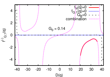
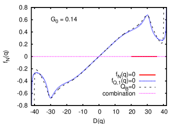
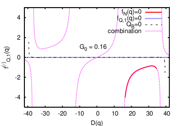
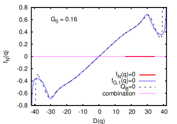
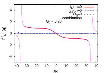
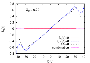
Figure 5: Gauge dependent quantities, $f^{(-)}_{Q,1}(q)$ (left column) and $f_{N}(q)$ (right column), plotted as functions of the deformation $D$. The upper, middle and lower rows display the results for $G_{0}=0.14,0.16$ and $0.20$, respectively. See the caption of Fig. 4.

Figures 4 and 5 display the chemical potential $\lambda(q)$ and the quantities, $f^{(-)}_{Q,1}(q)$ and $f_{N}(q)$, respectively. Their values depend on the gauge adopted. If the QRPA gauge is used, $\lambda(q)$ should be constant along the path because of the condition $f_{N}(q)=B(q)\partial\lambda/\partial q=0$. We find, however, $\lambda(q)$ diverges near the inflection point of the collective potential where $\omega(q)^{2}=\partial^{2}V/\partial q^{2}=0$. This divergence occurs because the inflection point is a singularity for the gauge transformation (116) where an arbitrary $\alpha$ gives the same $f_{N}(q)$. Thus, the calculation using the QRPA gauge stops at the inflection point. On the other hand, we can go over the inflection point using the ETOP gauge, because the gauge transformation for $f^{(-)}_{Q,1}(q)$ (114) involves only the monopole pairing gap $\Delta_{0}(q)$ which always takes finite values along the collective path (except at the limit of the model space). In these figures we also present the results that are obtained by the following procedure: After determining the collective paths with the use of the ETOP gauge, we calculate the gauge-dependent quantities, $\lambda(q),f_{Q,1}^{(-)}(q)$, $f_{N}(q)$, by switching to the QRPA gauge using the relations

$$f^{(-)}_{Q,1({\rm QRPA})}= -\frac{4f_{N}(q)_{({\rm ETOP})}\Delta_{0}(q)}{\omega^{2}(q)}$$ (118a)

$$\lambda(q)_{({\rm QRPA})}= \lambda(q)_{({\rm ETOP})}-\frac{4f_{N}(q)_{({\rm ETOP})}}{\omega^{2}(q)}\frac{\partial V}{\partial q}$$ (118b)

We see in Figs. 4 and 5 that the results obtained by this procedure agree with those calculated by using the QRPA gauge ($f_{N}(q)=0$) from the beginning (in the region of deformation $D(q)$ where the collective path can be obtained using the QRPA gauge). This agreement demonstrates that the collective paths determined by using different gauge fixing conditions are the same, as it should be. Nevertheless, there is a suitable gauge fixing condition in finding solutions of the ASCC equations and constructing the collective path. For the multi-$O$(4) model with superfluidity, we find that the ETOP gauge is more useful than the QRPA gauge, because the gauge transformation (114) is well defined as long as the pairing gap $\Delta_{0}(q)$ is non-zero.

5.3 Comparison with the previous calculation

In our previous paper[57], we employed the ETOP gauge condition ($f^{(-)}_{Q,1}(q)=0$) but the $B$-part of $\hat{Q}(q)$ is ignored. Let us evaluate the error caused by this approximation. The results of such calculation are presented also in Figs. 1-4 and compared with those of the full calculation. We see that they agree well indicating that the approximation of ignoring the $B$-part is rather good.

In Fig. 5, we present the quantity

$$f^{(-)}_{Q,1}(q)=-\kappa_{s}\left\langle\phi(q)\right|[\hat{F}^{(-)}_{s},\hat{Q}(q)]\left|\phi(q)\right\rangle=-\kappa_{s}\sum_{i>0}Q^{A}_{i}(q)$$ (119)

evaluated using the $\hat{Q}(q)$ operator that is obtained by ignoring the $B$-part in the process of solving the ASCC equations. This quantity should be zero if the $\hat{Q}(q)$ operator determined by the gauge-invariant ASCC equations is used. We see that the deviation from zero is negligible (except near the limit of the model space), again indicating that the approximation is good.

The quantum spectra and transition strengths are displayed in Fig. 6. These are obtained by solving the Schrödinger equation for the quantized collective Hamiltonian. In this figure, effects of the quadrupole pairing interaction are also shown. We see that the results of the previous calculation (in which the $B$-part of $\hat{Q}(q)$ is ignored) are quite similar to those of full calculation (including the $B$-part), and both results well reproduce the trend of the excitation spectra obtained by exact diagonalization of the microscopic Hamiltonian (Fig. 7). The numerical calculation presented above thus suggest that the approximation of ignoring the $B$-part of $\hat{Q}(q)$, adopted in our previous paper[57], is justified and it may serve as an economical way of determining the collective path.

6 Concluding Remarks

We have shown that the basic equations of the ASCC method are invariant against transformations involving the angle in the gauge space conjugate to the particle-number. By virtue of this invariance, a clean separation between the large-amplitude collective motion and the pairing rotational motion can be achieved, enabling us to restore the particle-number symmetry broken by the HFB approximation. We have formulated the ASCC method explicitly in a gauge-invariant form, then, applied it to the multi-$O$(4) model using different gauge-fixing procedures. The calculations using different gauges indeed yield the same results for gauge-invariant quantities, such as the collective path, the collective mass parameter, and spectra obtained by the requantization of the collective Hamiltonian. We have suggested a gauge-fixing prescription that can be used in realistic calculations.

The explicit gauge invariance requires a $B$-part ($a^{\dagger}a$ part) of the collective coordinate operator $\hat{Q}(q)$. Actually, Ref. nak00 remarks that the separation of the Nambu-Goldstone modes in the local harmonic formulation requires higher-order terms in the collective coordinate. This is consistent with the present conclusion in the gauge-invariant formalism. We have also demonstrated that the approximation to neglect the $B$-part leads to results almost identical to those of the full calculation, at least for the multi-$O(4)$ model.

We are now investigating the oblate-prolate shape coexistence phenomena [54, 55, 56] in nuclei around ⁶⁸Se using the pairing-plus-quadrupole interactions [63, 64, 65] using the prescription on the basis of the new formulation of the ASCC method proposed in this paper. The result will be reported in a near future.

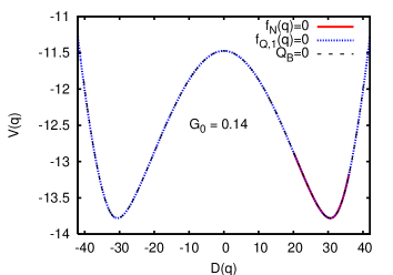
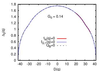
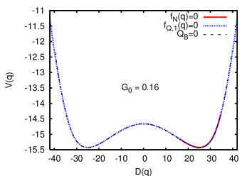
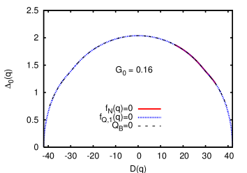
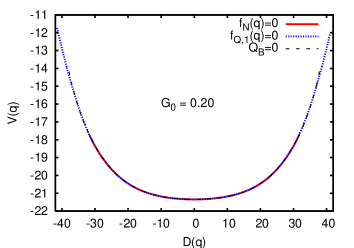
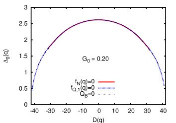
Figure 1: Collective potentials $V(q)$ and monopole pairing gaps $\Delta_{0}(q)$ plotted as functions of the quadrupole deformation $D$. The upper, middle and lower panels display the results for $G_{0}=0.14,0.16$ and $0.20$, respectively. In each column, results of different calculation are compared; those obtaind using the QRPA gauge ($f_{N}(q)=0$) and the ETOP gauge ($f^{(-)}_{Q,1}(q)=0$) are plotted by solid (red) and dotted (blue) lines, respectively, while those obtaind ignoring the $B$-part of $\hat{Q}(q)$ (i.e., putting $Q_{i}^{B}(q)=0$) by dashed lines.

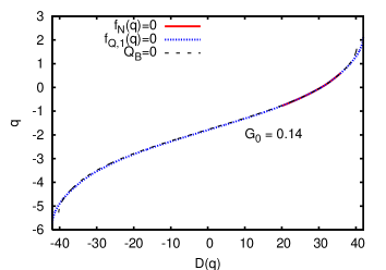
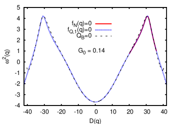
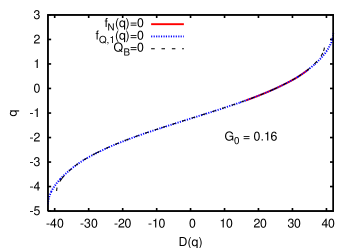
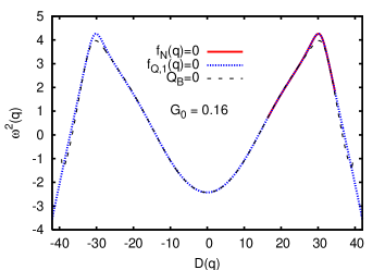
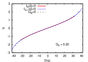
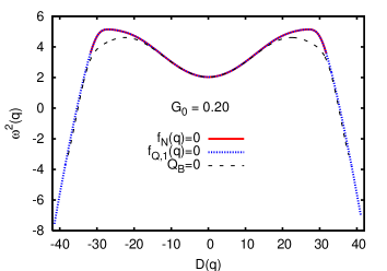
Figure 2: Left column: Relation between the collective coordinate $q$ and the quadrupole deformation $D(q)=\left\langle\phi(q)\right|\hat{D}\left|\phi(q)\right\rangle$. The point $q=0$ corresponds to the HFB equilibrium, which is the starting point of the numerical calculation. Right column: Squared frequencies $\omega^{2}(q)$ of the local harmonic equations, plotted as functions of $D$. Note that they are negative; i.e., $\omega(q)$ is purely imaginary in the region where the curvature of the collective potential is negative. The upper, middle and lower rows display the results for $G_{0}=0.14,0.16$ and $0.20$, respectively. See the caption of Fig. 1.

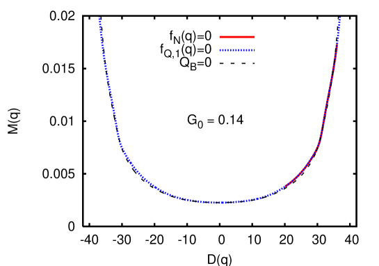
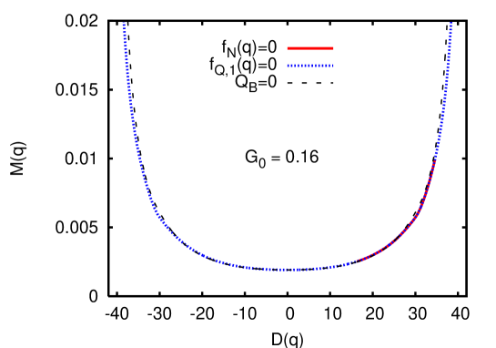
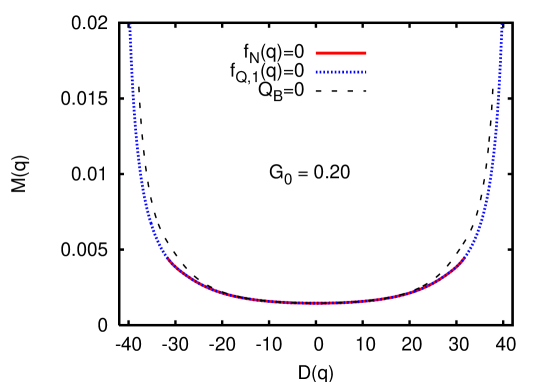
Figure 3: The ASCC collective mass $M(q(D))$ as functions of the deformation $D$. The upper, middle and lower rows display the results for $G_{0}$ = 0.14, 0.16 and 0.20, respectively. See the caption of Fig. 1.

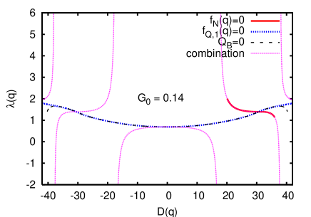
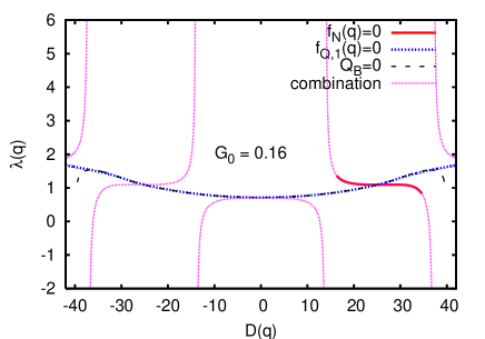
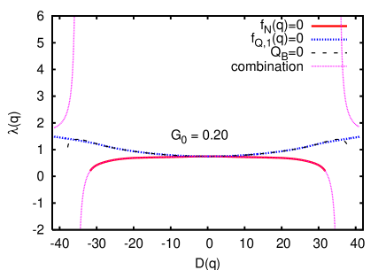
Figure 4: The chemical potentials $\lambda(q)$ as functions of the deformation $D$. The upper, middle and lower rows display the results for $G_{0}$ = 0.14, 0.16 and 0.20, respectively. In each column, results of different calculation are compared; The solid (red) and dotted (blue) lines indicate the results obtaind using the QRPA gauge ($f_{N}(q)=0$) and the ETOP gauge ($f^{(-)}_{Q,1}(q)=0$), respectively, while the dashed lines indicate those obtaind using the ETOP gauge but ignoring the $B$-part of $\hat{Q}(q)$ (i.e., putting $Q_{i}^{B}(q)=0$). The dotted (purple) lines labeled “combination” indicate the results calculated by switching to the QRPA gauge after the collective path is determined by using the ETOP gauge.

Figure 6: Excitation spectra and quadrupole transition matrix elements. left column: The result obtaind using the ETOP gauge ($f^{(-)}_{Q,1}(q)=0$) but ignoring the $B$-part of the collective coordinate operator $\hat{Q}(q)$. This is the same as presented in Ref. hin06.  right column: The result obtained by solving the gauge-invariant ASCC equations using the ETOP gauge. The upper, middle and lower rows display the results for $G_{0}$ = 0.14, 0.16 and 0.20, respectively. In each row, the results for $G_{2}=0.00,0.02$ and $0.04$ are compared. The numbers adjacent to the vertical lines are the absolute values of the transition matrix elements. The matrix elements between the doublets are indicated beside them.

Figure 7: Excitation spectra calculated with the exact diagonalization of the multi-$O(4)$ model Hamiltonian. The upper, middle and lower rows display the results for $G_{0}$ = 0.14, 0.16, and 0.20, respectively. In each row, the results for $G_{2}=0.00,0.02,0.04$ are compared. The numbers adjacent to vertical lines indicate the transition matrix elements. The matrix elements between the doublets are indicated beside them.

References

- [1] D. J. Rowe and R. Bassermann, Canad. J. Phys. 54 (1976), 1941.
- [2] D. M. Brink, M. J. Giannoni and M. Veneroni, Nucl. Phys. A 258 (1976), 237.
- [3] F. Villars, Nucl. Phys. A 285 (1977), 269.
- [4] T. Marumori, Prog. Theor. Phys. 57 (1977), 112.
- [5] M. Baranger and M. Veneroni, Ann. of Phys. 114 (1978), 123.
- [6] K. Goeke and P.-G. Reinhard, Ann. of Phys. 112 (1978), 328.
- [7] T. Marumori, T. Maskawa, F. Sakata and A. Kuriyama, Prog. Theor. Phys. 64 (1980), 1294.
- [8] M. J. Giannoni and P. Quentin, Phys. Rev. C 21 (1980), 2060; Phys. Rev. C 21 (1980), 2076.
- [9] J. Dobaczewski and J. Skalski, Nucl. Phys. A 369 (1981), 123.
- [10] K. Goeke, P.-G. Reinhard, and D. J. Rowe, Nucl. Phys. A 359 (1981), 408.
- [11] A. K. Mukherjee and M. K. Pal, Phys. Lett. B 100 (1981), 457; Nucl. Phys. A 373 (1982), 289.
- [12] D. J. Rowe, Nucl. Phys. A 391 (1982), 307.
- [13] C. Fiolhais and R. M. Dreizler, Nucl. Phys. A 393 (1983), 205.
- [14] P.-G. Reinhard, F. Grümmer and K. Goeke, Z. Phys. A 317 (1984), 339.
- [15] A. Kuriyama and M. Yamamura, Prog. Theor. Phys. 70 (1983), 1675; 71 (1984) 122.
- [16] M. Yamamura, A. Kuriyama and S. Iida, Prog. Theor. Phys. 71 (1984), 109.
- [17] M. Matsuo and K. Matsuyanagi, Prog. Theor. Phys. 74 (1985), 288.
- [18] M. Matsuo, Prog. Theor. Phys. 76 (1986), 372.
- [19] Y. R. Shimizu and K. Takada, Prog. Theor. Phys. 77 (1987), 1192.
- [20] M. Yamamura and A. Kuriyama, Prog. Theor. Phys. Suppl. No. 93 (1987).
- [21] A. Bulgac, A. Klein, N. R. Walet and G. Do Dang, Phys. Rev. C 40 (1989), 945.
- [22] N. R. Walet, G. Do Dang, and A. Klein, Phys. Rev. C 43 (1991), 2254.
- [23] A. Klein, N. R. Walet and G. Do Dang, Ann. of Phys. 208 (1991), 90.
- [24] K. Kaneko, Phys. Rev. C 49 (1994), 3014.
- [25] T. Nakatsukasa and N. R. Walet, Phys. Rev. C 57 (1998), 1192.
- [26] T. Nakatsukasa and N. R. Walet, Phys. Rev. C 58 (1998), 3397.
- [27] T. Nakatsukasa, N. R. Walet and G. Do Dang, Phys. Rev. C 61 (1999), 014302.
- [28] J. Libert, M. Girod and J.-P. Delaroche, Phys. Rev. C 60 (1999), 054301.
- [29] E. Kh. Yuldashbaeva, J. Libert, P. Quentin and M. Girod, Phys. Lett. B 461 (1999), 1.
- [30] L. Próchniak, P. Quentin, D. Samsoen and J. Libert, Nucl. Phys. A 730 (2004), 59.
- [31] D. Almehed and N. R. Walet, Phys. Rev. C 69 (2004), 024302.
- [32] D. Almehed and N. R. Walet, Phys. Lett. B 604 (2004), 163.
- [33] A. Klein and E. R. Marshalek, Rev. Mod. Phys. 63 (1991), 375.
- [34] G. Do Dang, A. Klein, and N. R. Walet, Phys. Rep. 335 (2000), 93.
- [35] A. Kuriyama, K. Matsuyanagi, F. Sakata, K. Takada and M. Yamamura (Ed.), Prog. Theor. Phys. Suppl. No. 141 (2001).
- [36] P. Ring and P. Schuck, The Nuclear Many-Body Problem (Springer-Verlag, 1980).
- [37] J.-P. Blaizot and G. Ripka, Quantum Theory of Finite Systems (The MIT press, 1986).
- [38] (Ed.) A. Abe and T. Suzuki, Prog. Theor. Phys. Suppl. Nos. 74 &75 (1983).
- [39] D. M. Brink and R. A. Broglia, Nuclear Superfluidity, Pairing in Finite Systems (Cambridge University Press, 2005).
- [40] M. Matsuo, Prog. Theor. Phys. 72 (1984) 666.
- [41] M. Matsuo and K. Matsuyanagi, Prog. Theor. Phys. 74 (1985) 1227; Prog. Theor. Phys. 76 (1986), 93; Prog. Theor. Phys. 78 (1987), 591.
- [42] M. Matsuo, Y. R. Shimizu and K. Matsuyanagi, Proceedings of The Niels Bohr Centennial Conf. on Nuclear Structure, ed. R. Broglia, G. Hagemann and B. Herskind (North-Holland, 1985), p. 161.
- [43] K. Takada, K. Yamada and H. Tsukuma, Nucl. Phys. A 496 (1989), 224.
- [44] K. Yamada, K. Takada and H. Tsukuma, Nucl. Phys. A 496 (1989), 239.
- [45] K. Yamada and K. Takada, Nucl. Phys. A 503 (1989), 53.
- [46] H. Aiba, Prog. Theor. Phys. 84 (1990), 908.
- [47] K. Yamada, Prog. Theor. Phys. 85 (1991), 805; Prog. Theor. Phys. 89 (1993), 995.
- [48] J. Terasaki, T. Marumori and F. Sakata, Prog. Theor. Phys. 85 (1991), 1235.
- [49] J. Terasaki, Prog. Theor. Phys. 88 (1992), 529; Prog. Theor. Phys. 92 (1994), 535.
- [50] M. Matsuo, in New Trends in Nuclear Collective Dynamics, ed. Y. Abe, H. Horiuchi and K. Matsuyanagi, (Springer-Verlag, 1992), p.219.
- [51] Y. R. Shimizu and K. Matsuyanagi, Prog. Theor. Phys. Suppl. No. 141 (2001), 285.
- [52] M. Matsuo, T. Nakatsukasa and K. Matsuyanagi, Prog. Theor. Phys. 103 (2000), 959.
- [53] M. Kobayasi, T. Nakatsukasa, M. Matsuo and K. Matsuyanagi, Prog. Theor. Phys. 112 (2004), 363; Prog. Theor. Phys. 113 (2005), 129.
- [54] J. L. Wood, K. Heyde, W. Nazarewicz, M. Huyse and P. van Duppen, Phys. Rep. 215 (1992), 101.
- [55] S. M. Fischer et al., Phys. Rev. Lett. 84 (2000), 4064; Phys. Rev. C 67 (2003), 064318.
- [56] E. Bouchez et al., Phys. Rev. Lett. 90 (2003), 082502.
- [57] N. Hinohara, T. Nakatsukasa, M. Matsuo and K. Matsuyanagi, Prog. Theor. Phys. 115 (2006) 567.
- [58] K. Matsuyanagi, Prog. Theor. Phys. 67 (1982), 1441; Proceedings of the Nuclear Physics Workshop, Trieste, 5-30 Oct. 1981. ed. C. H. Dasso, R. A. Broglia and A. Winther (North-Holland, 1982), p. 29.
- [59] Y. Mizobuchi, Prog. Theor. Phys. 65 (1981), 1450.
- [60] T. Suzuki and Y. Mizobuchi, Prog. Theor. Phys. 79 (1988), 480.
- [61] T. Fukui, M. Matsuo and K. Matsuyanagi, Prog. Theor. Phys. 85 (1991), 281.
- [62] M. Kobayasi, T. Nakatsukasa, M. Matsuo and K. Matsuyanagi, Prog. Theor. Phys. 110 (2003), 65.
- [63] M. Baranger and K. Kumar, Nucl. Phys. 62 (1965) 113; Nucl. Phys. A 110 (1968), 529; Nucl. Phys. A 122 (1968), 241; Nucl. Phys. A 122 (1968), 273.
- [64] M. Baranger and K. Kumar, Nucl. Phys. A 110 (1968), 490.
- [65] D. R. Bes and R. A. Sorensen, Advances in Nuclear Physics vol. 2, (Prenum Press, 1969), p. 129.