Shell-model study of mirror nuclei with modern charge-dependent NN potential

Abstract

The properties of $T=1/2$ mirror nuclei in the $fp$ shell have been studied with a microscopic residual interaction. The isospin-nonconserving interaction is derived from a high-precision charge-dependent Bonn NN potential using the folded-diagram renormalization method. The level structures of the nuclei are calculated, obtaining excellent agreements with experimental observations till the $0f_{7/2}$ band termination. The role played by isospin symmetry breaking on ground-state displacement energies and mirror energy differences is discussed, which may help to explain the long-standing Nolen-Schiffer anomaly. Electromagnetic and weak transition properties are presented, with discussions on the asymmetry in analogous transitions.

I Introduction

The investigation of mirror nuclei along the $N=Z$ line is of significant interest since it addresses directly the isospin symmetry problem in nuclear many-fermion systems. Isospin symmetry is approximate due to the charge dependence in strong force and the Coulomb force between protons. Direct evidence of isospin symmetry breaking (ISB) can be deduced from ground-state displacement energies (MDE) and excitation-energy differences between analogous states (MED) in mirror nuclei. In the past decade, numerous experimental and theoretical efforts have been devoted to mirror pairs in the lower $fp$ shell and extends the knowledge of MED evolution patterns to high-spin states Zuker02 ; Martinezpinedo97 ; Brandolini05 ; Poves01 ; Bentley00 ; Bentley06 ; Bentley98 ; Oleary97 ; Tonev02 ; William03 .

The MDE range from a few to tens of MeV, with the dominant origin in the Coulomb field Shlomo78 . However, if only the Coulomb effect is considered, a persistent inaccuracy exists between the theoretical results of MDE and corresponding experimental observations ns . This long-standing problem is referred to as Nolen-Schiffer anomaly ns , revealing the necessity to introduce charge symmetry breaking (CSB) in strong force in depicting nuclear properties Miller90 ; Suzuki92 ; Brown00 ; Machleidt01 ; Muther99 ; Tsushima99 . Contributions from the Coulomb field and CSB in strong force to MED has been shown theoretically, e.g., in Ref. Zuker02 , finding that the later is at least as important as the former.

The purpose of this work is to study the structures and decay properties of $T=1/2$ mirror nuclei in the lower fp shell by shell-model diagonalization method and to investigate the effects of ISB. We employ an isospin-nonconserving effective Hamiltonian interaction derived microscopically from a high-precision version of the charge-dependent Bonn (CD-Bonn) nucleon-nucleon (NN) potential Machleidt01 using the folded-diagram renormalization method Kuo90 ; Jensen95 . The charge dependence of the NN interaction is retained, enabling to quantify its effect on nuclear properties exactly with full model-space diagonalizations. In our previous work, the effective Hamiltonian has been used to study the isospin structures of odd-odd $N=Z$ nuclei in the lower fp shell interaction .

The essence of the shell model lies in that the true eigen energies and wave functions of the original many-body Hamiltonian can be constructed by diagonalizing an effective Hamiltonian in a constrained finite model space Towner ; Kuo90 . The model-space dependent effective Hamiltonian can be written as

$$H_{\text{eff}}=H_{\text{o}}^{\prime}+v_{\text{eff}},$$ (1)

where $H_{\text{o}}^{\prime}=\sum_{\alpha}\varepsilon_{\alpha}^{\prime}\text{a}^{{\dagger}}_{\alpha}\text{a}_{\alpha}$ is the effective one-body Hamiltonian with $\varepsilon_{\alpha}^{\prime}$ being single-particle energies (SPE). In general calculations, the effective interaction $v_{\text{eff}}$ is expressed as two-body matrix elements (TBME) in harmonic oscillator (HO) basis. The effective interaction can be decomposed into two parts. The monopole part of the interaction, in combination with the SPE, gives out the bulk properties of the nuclei. The multipole part of the effective interaction accounts for the configuration-mixing which is essential for modern shell-model calculations Caurier05 .

The effective interaction is directly related to the underlying NN potential. Due to the unperturbative nature of the QCD at low energies, most of the knowledge concerning the NN force is from the measurements of nucleon-nucleon and nucleon-deuteron scattering properties. The scattering behavior can be well approximated by one-boson-exchange (OBE) potential which has been commonly employed in modern realistic NN forces Machleidt01 . The bare NN potential, however, is unsuitable for direct applications in nuclear systems due to the strong repulsive core. In early practices, the Brueckner G reaction matrix is introduced to evaluate the effective interaction for a chosen model space, as done in the derivation of the famous Kuo-Brown interaction Kuo68 . The G matrix takes into account the short-range repulsive behavior of the NN potential and satisfies

$$\langle\Psi|G|\Psi\rangle=\langle\Psi|V|\Psi\rangle,$$ (2)

where $V$ is the bare $NN$ potential and $|\Psi\rangle$ the correlated wave function.

Effective interaction with the G matrix may lead to bad behavior with increasing particle numbers. The folded-diagram renormalization method is proposed to include the core-polarization effect from the configuration-mixing outside the model space. Folded and non-folded diagrams are introduced in evaluating the time-evolution operator in time-dependent perturbation theory in which both contributions from the model space and the excluded space are considered. The two kinds of diagrams can be evaluated from the G matrix.

In 1990s, various high-precision phenomenological OBE potentials (e.g., AV18 of the Argonne group, Nijm I $\&$ II of the Nigmegen group and CD-Bonn of the Bonn group) have been proposed by fitting the huge amount of neutron-proton and proton-proton scattering data available Machleidt01 , with reasonable descriptions of the charge dependence in strong force. Both charge independence and charge symmetry are related to the symmetric properties of the $NN$ force under rotations in isospin space. The breaking of charge symmetry and charge independence are mainly due to the mass splitting of the nucleons (m${}_{\text{proton}}\neq$ m${}_{\text{neutron}}$) and pions (m${}_{\pi^{\pm}}\neq$ m${}_{\pi^{0}}$). CSB is a special case of CIB, referring to the difference between the proton-proton and neutron-neutron interactions. CIB means that all interactions in isospin $T=1$ state, the proton-proton, neutron-neutron and neutron-proton interactions, are different, after electromagnetic effects have been removed.

All the OBE potentials have similar low-momentum behavior. In the present work, we use a new high-precision CD-Bonn potential. Detailed descriptions on the CD-Bonn potential can be found in Ref. Machleidt01 . In the CD-Bonn potential, both CSB and CIB are embedded in all partial waves with angular momentum $J\leq 4$. The off-shell behavior of the nonlocal covariant Feynman amplitudes used in the potential can lead to larger binding energies for nuclear many-body systems, which can help to improve the effective interaction’s performance around the $N=28$ shell closure KB3 .

II Level structures

The level structures of $T=1/2$ mirror nuclei in the lower $fp$ shell are calculated with the residual interaction described above (denoted as CD-Bonn). For comparison, the isospin-conserving KB3 interaction KB3 is also used. KB3 is a revised version of the Kuo-Brown interaction with monopole centroids modified to improve its performance around ⁵⁶Ni KB3 . The effective Hamiltonians are diagonalized with the shell model code OXBASH Oxbash . Calculations are performed in the $fp$ major shell. Specific center-of-mass corrections due to the effects of spurious states can be avoided Dean04 . Earlier theoretical efforts on the nuclei can be find, e.g., in Refs. Brandolini05 ; Poves01 ; Martinezpinedo97 .

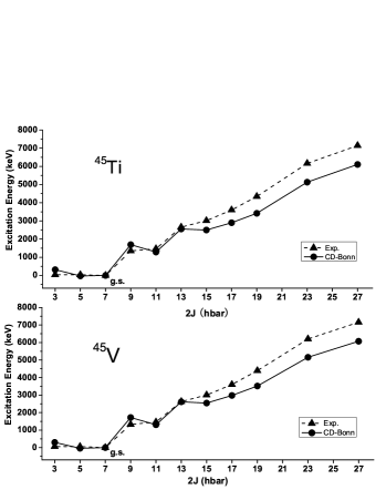
Figure 1: Experimental and calculated excitation energies for yrast bands in ⁴⁵Ti and ⁴⁵V. Experimental results are taken from Ref. Bentley06

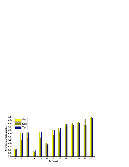
Figure 2: Average number of particles in the $0f_{7/2}$ sub-shell for yrast states in ⁴⁵Ti and ⁴⁵V. Columns denoted by ⁴⁵Ti and ⁴⁵V are results calculated with the CD-Bonn interaction.

Fig. 1 shows the calculated excitation energies of yrast bands in ⁴⁵V and ⁴⁵Ti, together with experimental observations Bentley06 . Agreements between calculations and experiments are satisfactory. Experiments have identified three low-lying states with $J^{\pi}=7/2^{-},~{}5/2^{-}$ and $3/2^{-}$. In the framework of the deformed Nilsson model, the structure can be interpreted as the splitting of the $0f_{7/2}$ harmonic oscillator orbit into $[321]3/2^{-},~{}[312]5/2^{-}$ and $[303]7/2^{-}$ orbits at low excitation energies. The existence of these nearly-degenerate states gives evidence for nuclear deformation. In spherical shell model, deformation is described as configuration-mixing contribution from upper sub-shells. The configuration of $3/2^{-}$ state can be approximately described as the excitation of one particle out of the $0f_{7/2}$ orbit, as shown in Fig. 2, in which the $0f_{7/2}$ occupancies for ⁴⁵V and ⁴⁵Ti are plotted as a function of spin.

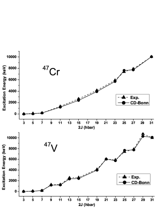
Figure 3: Same as Fig. 1 but for ⁴⁷V and ⁴⁷Cr. Experimental results are taken from Ref. Bentley98 ; Tonev02

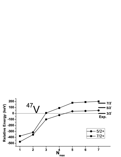
Figure 4: The sequence of the ground-state triplet under different model truncations. $\text{N}_{\text{max}}$ denotes the maximal number of particles being excited to the upper $fp$ shell.

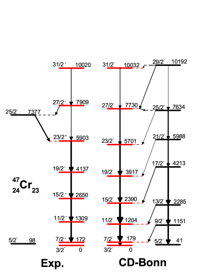
Figure 5: Experimental and proposed yrast band for ⁴⁷Cr.

For nuclei with $A\geq 47$, excellent agreements between calculations and experiments are obtained. Theoretical and experimental results for mirror pair ⁴⁷V and ⁴⁷Cr are shown in Fig. 3. The nucleus ⁴⁷V has been recognized as a $K=3/2$ rotor. Our calculations show that the contribution from the upper $fp$ shell plays an important role in giving the correct positions of the $3/2^{-}$ ground state and other low-lying states. In Fig. 4 we plotted the evolution of the relative positions of the ground-state triplet as a function of the maximal number of particles ($\text{N}_{\text{max}}$) being excited out of the $0f_{7/2}$ sub-shell. To give the correct $3/2^{-}$ ground state, $\text{N}_{\text{max}}$ must be larger than four to account for the configuration mixing. This configuration corresponds to a prolate deformation. Also interesting is the nearly degenerate coupled doublet in the yrast band of ⁴⁷V Brandolini01 . Calculations reproduce well the relative sequence of the yrast states. A similar scheme is predicted for ⁴⁷Cr, as shown in Fig. 5.

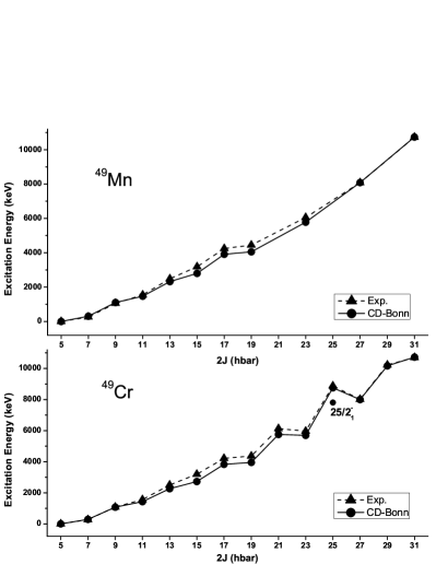
Figure 6: Same as Fig. 1 but for ⁴⁹Cr and ⁴⁹Mn. Experimental data are taken from Ref. Oleary97 .

Calculated results for mirror pairs ⁴⁹Cr-⁴⁹Mn and ⁵¹Mn-⁵Fe are shown in Fig. 6 and 7, respectively. Calculations are done in truncated $fp$ model spaces. These two pairs are the cross-conjugate partners of the $A=47$ and $A=45$ nuclei, respectively. For nucleus ⁴⁹Cr, one $25/2^{-}$ state with an excitation energy of 8879 keV was observed in Ref. Oleary97 . The calculated level most close to the observed state locates at 8758 keV. In our calculations, four $25/2^{-}$ states are generated around 8879 keV, with the lowest one lying at 7812 keV. The proposed yrast state is more close to the experimental result of 8334 keV given in Ref. Brandolini01 . However, confusion still exists concerning the calculated B(E2) for the $25/2_{1}^{-}\rightarrow 21/2_{1}^{-}$ transition when comparing with the corresponding experimental result, which will be discussed below.

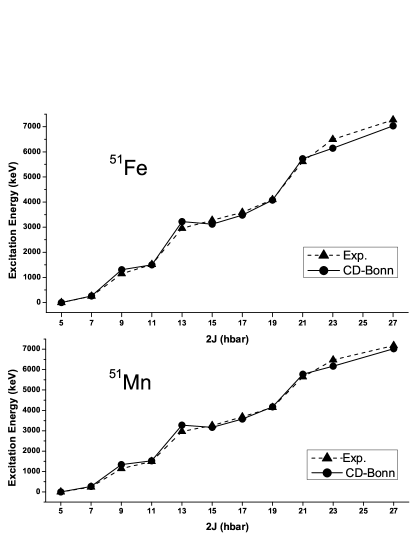
Figure 7: Same as Fig. 1 but for ⁵¹Fe and ⁵¹Mn. Experimental data are taken from Ref. Bentley00 .

Our calculations in the $fp$ shell generate well the negative-parity bands for the odd-A nuclei. Positive-parity states can be approximated by assuming a hole in the $0d_{3/2}$ orbit. In nuclei ⁴⁵Ti and ⁴⁵V, the positive-parity collective bands start at 328 keV and 386 keV, respectively. To give a good description of the positive-parity states, large-scale calculation in full $sdpf$ shell is needed Brandolini05 . However, it is beyond the scope of this paper.

III ISB effects in MDE and MED

As mentioned above, the discrepancy between the theoretical MDE of mirror nuclei and corresponding experimental data is a long-standing problem in nuclear physics Shlomo78 ; ns ; Suzuki92 . In Ref. Brown00 , Brown et al. investigated the role played by CSB in addressing the NS anomaly in a self-consistent Hartree-Fock method by adding a CSB term to the $s$-wave part of the Skyrme interaction. The crucial importance of introducing CSB in partial waves with $L>0$ for the full explanation of the NS anomaly have been further studied by Müther et al. within the Bruckner-Hartree-Fock calculations of nuclear matter Muther99 . The anomaly has also been investigated by Tsushima et al. Tsushima99 at the quark level using the so-called quark-meson coupling (QMC) model in which the mass-difference between the up and down quark is taken into account. QMC can be seen as an extended model of the relativistic mean-field theory with quark mass difference entering to account for the short-range CSB Miller90 .

Table 1: $0f_{7/2}$-$0f_{7/2}$ monopole interactions and the monopole centroids. The $T=1$ KB3 matrix elements are also shown for a comparison.

$j$	0	2	4	6	centroid
$\pi-\pi$	-1.22	-0.20	0.58	0.86	0.51
$\nu-\nu$	-1.54	-0.39	0.40	0.69	0.32
KB3	-1.92	-1.09	-0.19	0.18	-0.24

Table 2: ISB contribution (in MeV) to MDE. See details in the text.

Mirror pair	A=45	A=47	A=49	A=51
T=1/2	0.359	0.604	0.658	0.936
T=3/2	1.269	1.586	2.197	2.579

In isospin-conserving shell-model calculations, the binding energies of mirror nuclei are identical since the Coulomb field is not taken into account. In this work, the Coulomb force and charge-dependence in strong force are embedded at the two-body level, as shown in Table 1. The two-body ISB interaction leads to more binding energies for the neutron-rich side of the mirror nuclei. The binding-energy differences of $T=1/2$ mirror pairs are of the order of a few hundreds keV. Table 2 shows results for $T=1/2$ and $T=3/2$ mirror pairs which is defined as

$$\Delta E_{ISB}=E(Z_{<},\text{g.s.})-E(Z_{>},\text{g.s.}),$$ (3)

where $Z_{<}~{}(Z_{>})$ denotes neutron (proton)-rich side of mirror nuclei. The energy differences reflect contribution from ISB to MDE. What is still absent in the present Hamiltonian is the proper evaluation of Coulomb effect on the SPE. The study of Coulomb effect on MDE in the context of the shell model has been shown, i.e., in Ref Ormand97 . Further investigations of the problem would be done in the future to see whether the charge-dependent strong force can be totally responsible for the NS anomaly.

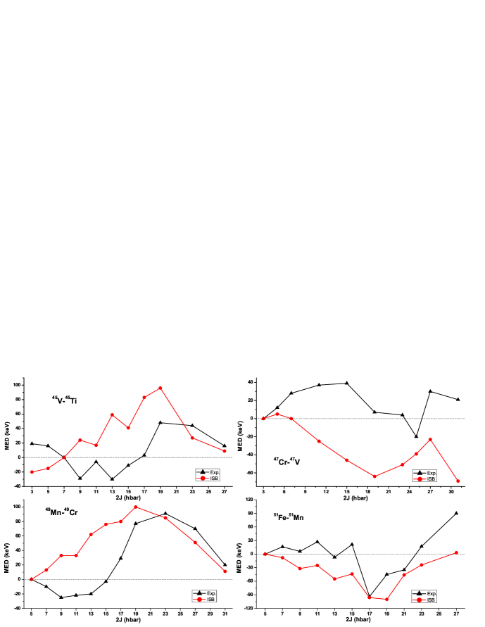
Figure 8: $\Delta V_{M}$ contribution (denoted as ISB) to MED for $T=1/2$ mirror pairs ⁴⁵Ti-⁴⁵V, ⁴⁷V-⁴⁷Cr, ⁴⁹Cr-⁴⁹Mn and ⁵¹Mn-⁵¹Fe. Experimental data are taken from Ref. Bentley00 ; Bentley06 ; Bentley98 ; Oleary97 ; Tonev02 . See the text for details.

In medium-mass nuclei, observed MED are very small (usually of the order of 10-100 keV) Zuker02 . It provides a special ground to deduce the effect of charge-dependent strong force. In Ref. Zuker02 , contribution from CSB are approximated by an additional $J=2$ pairing term evaluated phenomenally from the MED and triplet energy difference in the A=42 isospin triplet. Contributions from the Coulomb field and the above CSB term were collected and compared with the measured MED in ⁴⁵V and ⁴⁵Ti by Bentley et al. Bentley06 . However, the prediction power of the model is very poor Bentley06 , indicating that a more precise treatment of the charge-dependence in strong force is needed.

In the present work, contributions from the two-body Coulomb force and the charge-dependent strong force can be calculated exactly from the calculated energy differences of analogous states in mirror nuclei. We simply decompose the contributions to total MED into two parts,

$$\text{MED}_{J}=\Delta\langle U_{s}\rangle_{J}+\Delta(V_{M})_{J},$$ (4)

where $\Delta\langle U_{s}\rangle_{J}$ denotes contribution from the Coulomb shifts of proton SPE. $\Delta(V_{M})_{J}$ is given as

$$\Delta(V_{M})_{J}=E_{\text{cal.}}(Z_{>})_{J}-E_{\text{cal.}}(Z_{<})_{J},$$ (5)

where $E_{\text{cal.}}$ is calculated excitation energy of the state with angular momentum $J$. Calculations for $\Delta(V_{M})_{J}$ are plotted in Fig. 8.

Configurations for low-lying states in the lower $fp$ shell nuclei are dominated by the $0f_{7/2}$ orbit since a sizable energy-gap between the $0f_{7/2}$ and other orbits ($1p_{3/2},0f_{5/2},1p_{1/2}$) exists. Contributions from the monopole part of the Coulomb force, however, are sensitive to the $1p_{3/2}$ occupancy and are expected to be enhanced at the nuclear surface Bulgac99 . In recent studies, explanations of the evolution behavior of MED with spin have been focus on particle alignment and nuclear shape changes Bentley00 ; Oleary97 ; Bentley98 . These arguments are mainly based on the fact that the MED tend to vanish at band termination states where maximum possible alignments of all valence particles are expected.

In the MED of the $A=51$ mirror pair, two sharp changes exist, leading to two peaks of about 100 keV at the $J=17/2^{-}$ state and the band-terminated $J=27/2^{-}$ state. Calculations with empirical Coulomb matrix elements reproduced the two peaks but over-estimated results for the $J=17/2^{-}$ state Bentley00 . Further investigations by the authors showed that a sharp alignment of a $0f_{7/2}$ proton pair exist at the $17/2^{-}$ state in ⁵¹Fe Bentley00 . In our calculations, the ISB contribution $\Delta(V_{M})_{J}$ reproduced the peak at the $J=17/2^{-}$ state and vanished at the termination state.

Also interesting is the staggering in the MED of yrast bands in mirror pair ⁴⁵Ti and ⁴⁵V and the cross-conjugate partners ⁵¹Fe and ⁵¹Mn. In Ref. Bentley00 , it was tentatively explained as the existence of two bands with different signatures in the yrast band. Calculated $\Delta(V_{M})_{J}$ characterized the staggering.

IV Transition properties in mirror nuclei

Electromagnetic (EM) and Gamow-Teller (GT) analogous transitions in mirror nuclei can provide other detailed information on the properties of nuclear structures and transition operators Ekman04 ; Fujita04 ; Smirnova03 . Different transition strengths have already been identified in the yrast cascades of ⁴⁷V and ⁴⁷Cr, with tentative work trying to extract information on differences in corresponding wave functions by Tonev et al. Tonev02 . In the following, calculated strengths for EM and GT analogous transitions will be given, with the analyse of existing asymmetries.

Table 3: Calculated B(E2) (in e²fm⁴) in mirror nuclei ⁴⁵Ti and ⁴⁵V. Effective charges with e_p=1.5e and e_n=0.5e are used.

	45Ti					45V
$J_{i}\rightarrow J_{f}$	HO	WS	SKcsb	KB3		HO	WS	SKcsb	KB3
$11/2^{-}_{1}\rightarrow 7/2^{-}_{1}$	124	124	105	132		154	158	134	157
$15/2^{-}_{1}\rightarrow 11/2^{-}_{1}$	139	139	118	144		167	171	146	165
$19/2^{-}_{1}\rightarrow 15/2^{-}_{1}$	96	95	80	94		110	113	95	98
$23/2^{-}_{1}\rightarrow 19/2^{-}_{1}$	65	64	54	70		119	122	104	118
$27/2^{-}_{1}\rightarrow 23/2^{-}_{1}$	48	47	40	50		87	90	76	83
$9/2^{-}_{1}\rightarrow 5/2^{-}_{1}$	82	86	71	94		97	101	85	104
$13/2^{-}_{1}\rightarrow 9/2^{-}_{1}$	151	160	131	158		175	185	155	191
$17/2^{-}_{1}\rightarrow 13/2^{-}_{1}$	100	101	84	108		130	135	113	130
$9/2^{-}_{1}\rightarrow 7/2^{-}_{1}$	48	51	41	83		41	45	36	77
$13/2^{-}_{1}\rightarrow 11/2^{-}_{1}$	33	35	29	44		28	30	25	31
$15/2^{-}_{1}\rightarrow 13/2^{-}_{1}$	16	17	14	22		30	33	26	27
$17/2^{-}_{1}\rightarrow 15/2^{-}_{1}$	14	14	12	22		9	10	8	11
$19/2^{-}_{1}\rightarrow 17/2^{-}_{1}$	17	17	15	17		38	40	34	30

Table 4: Theoretical B(M1) (in $\mu^{2}_{N}$) and B(GT) in mirror pair ⁴⁵Ti and ⁴⁵V. Free nucleon g-factors [g_s(proton)=5.586, g_s(neutron)=-3.826, g_l(proton)=1 and g_l(neutron)=0] and free axial-vector constant ($g_{A}=1.26$) are used.

	B(M1)			B(GT)
$J_{i}\rightarrow J_{f}$	45Ti	45V		$\beta^{+}$	CE
$9/2^{-}_{1}\rightarrow 7/2^{-}_{1}$	0.40	0.42		0.12	0.13
$13/2^{-}_{1}\rightarrow 11/2^{-}_{1}$	0.21	0.25		0.08	0.09
$15/2^{-}_{1}\rightarrow 13/2^{-}_{1}$	0.87	0.83		0.30	0.32
$17/2^{-}_{1}\rightarrow 15/2^{-}_{1}$	0.11	0.13		0.04	0.05
$19/2^{-}_{1}\rightarrow 17/2^{-}_{1}$	0.15	0.16		0.53	0.53

Table 3 shows calculated strengths for electrical quadrupole (E2) analogous transitions in ⁴⁵Ti and ⁴⁵V. Effective charges for neutrons and protons have been renormalized to e_n=0.5e and e_p=1.5e, respectively, to account for the core-polarization effect. The wave functions of the shell model are calculated with three different bases, i.e., the HO, the Woods-Saxon (WS) potential and the Skyrme force (SKcsb) by Brown et al. Brown00 in which a charge-symmetry-breaking term has been added. For comparison, results calculated with the KB3 interaction and the HO basis (denoted as KB3) are also shown.

Table 5: Calculated B(E2) (in e²fm⁴) and B(M1) (in $\mu^{2}_{N}$) for analogous transitions in mirror pair ⁴⁷V and ⁴⁷Cr.

	B(E2)		B(M1)
$J_{i}\rightarrow J_{f}$	47V	47Cr	47V	47Cr
$7/2^{-}_{1}\rightarrow 3/2^{-}_{1}$	142	172
$11/2^{-}_{1}\rightarrow 7/2^{-}_{1}$	242	314
$15/2^{-}_{1}\rightarrow 11/2^{-}_{1}$	249	326
$19/2^{-}_{1}\rightarrow 15/2^{-}_{1}$	203	261
$23/2^{-}_{1}\rightarrow 19/2^{-}_{1}$	182	221
$27/2^{-}_{1}\rightarrow 23/2^{-}_{1}$	118	141
$31/2^{-}_{1}\rightarrow 27/2^{-}_{1}$	67	96
$9/2^{-}_{1}\rightarrow 5/2^{-}_{1}$	182	248
$13/2^{-}_{1}\rightarrow 9/2^{-}_{1}$	220	291
$17/2^{-}_{1}\rightarrow 13/2^{-}_{1}$	218	256
$21/2^{-}_{1}\rightarrow 17/2^{-}_{1}$	185	225
$25/2^{-}_{1}\rightarrow 21/2^{-}_{1}$	121	141
$29/2^{-}_{1}\rightarrow 25/2^{-}_{1}$	1	1
$5/2^{-}_{1}\rightarrow 3/2^{-}_{1}$	314	393	0.15	0.13
$7/2^{-}_{1}\rightarrow 5/2^{-}_{1}$	251	282	0.29	0.26
$9/2^{-}_{1}\rightarrow 7/2^{-}_{1}$	101	137	0.11	0.10
$13/2^{-}_{1}\rightarrow 11/2^{-}_{1}$	43	60	0.07	0.06
$15/2^{-}_{1}\rightarrow 13/2^{-}_{1}$	74	81	0.70	0.62
$17/2^{-}_{1}\rightarrow 15/2^{-}_{1}$	17	25	0.03	0.03
$17/2^{-}_{1}\rightarrow 19/2^{-}_{1}$	37	49	0.70	1.0
$21/2^{-}_{1}\rightarrow 19/2^{-}_{1}$	2.4	8.3	0.11	0.12
$21/2^{-}_{1}\rightarrow 23/2^{-}_{1}$	2.9	5	1.6	1.5
$25/2^{-}_{1}\rightarrow 23/2^{-}_{1}$	0.06	2.7	0.06	0.07
$27/2^{-}_{1}\rightarrow 25/2^{-}_{1}$	4.1	6.2	2.2	2.1
$29/2^{-}_{1}\rightarrow 31/2^{-}_{1}$	0.24	0.10	0.27$\times 10^{-2}$	0.18$\times 10^{-2}$
$29/2^{-}_{1}\rightarrow 27/2^{-}_{1}$	5.4	18	0.10$\times 10^{-1}$	0.15$\times 10^{-1}$

Table 6: Theoretical B(E2) (in e²fm⁴) and B(M1) (in $\mu^{2}_{N}$) for analogous transitions in mirror pair ⁴⁹Cr and ⁴⁹Mn.

	B(E2)			B(M1)
$J_{i}\rightarrow J_{f}$	49Cr	49Mn		49Cr	49Mn
$9/2^{-}_{1}\rightarrow 5/2^{-}_{1}$	110	109
$13/2^{-}_{1}\rightarrow 9/2^{-}_{1}$	223	225
$17/2^{-}_{1}\rightarrow 13/2^{-}_{1}$	191	214
$21/2^{-}_{1}\rightarrow 17/2^{-}_{1}$	190	246
$25/2^{-}_{1}\rightarrow 21/2^{-}_{1}$	148	231
$29/2^{-}_{1}\rightarrow 25/2^{-}_{1}$	165	224
$11/2^{-}_{1}\rightarrow 7/2^{-}_{1}$	195	204
$15/2^{-}_{1}\rightarrow 11/2^{-}_{1}$	228	230
$19/2^{-}_{1}\rightarrow 15/2^{-}_{1}$	211	223
$23/2^{-}_{1}\rightarrow 19/2^{-}_{1}$	191	224
$27/2^{-}_{1}\rightarrow 23/2^{-}_{1}$	131	159
$31/2^{-}_{1}\rightarrow 27/2^{-}_{1}$	51	55
$7/2^{-}_{1}\rightarrow 5/2^{-}_{1}$	382	408		0.24	0.26
$9/2^{-}_{1}\rightarrow 7/2^{-}_{1}$	307	299		0.57	0.58
$11/2^{-}_{1}\rightarrow 9/2^{-}_{1}$	234	247		0.65	0.66
$13/2^{-}_{1}\rightarrow 11/2^{-}_{1}$	165	162		0.70	0.73
$15/2^{-}_{1}\rightarrow 13/2^{-}_{1}$	106	130		0.88	0.93
$17/2^{-}_{1}\rightarrow 15/2^{-}_{1}$	67	89		0.29	0.33
$19/2^{-}_{1}\rightarrow 17/2^{-}_{1}$	92	131		0.42	0.53
$21/2^{-}_{1}\rightarrow 19/2^{-}_{1}$	38	72		0.48$\times 10^{-1}$	0.63$\times 10^{-1}$
$25/2^{-}_{1}\rightarrow 23/2^{-}_{1}$	29	61		0.30$\times 10^{-3}$	0.68$\times 10^{-5}$
$29/2^{-}_{1}\rightarrow 27/2^{-}_{1}$	22	45		0.47$\times 10^{-2}$	0.64$\times 10^{-2}$
$31/2^{-}_{1}\rightarrow 29/2^{-}_{1}$	3.0	10		0.58	0.75

Table 7: Calculated B(E2) (in e²fm⁴) and B(M1) (in $\mu^{2}_{N}$) for analogous transitions in mirror pair ⁵¹Mn and ⁵¹Fe.

	B(E2)			B(M1)
$J_{i}\rightarrow J_{f}$	51Mn	51Fe		51Mn	51Fe
$9/2^{-}_{1}\rightarrow 5/2^{-}_{1}$	81	95
$13/2^{-}_{1}\rightarrow 9/2^{-}_{1}$	155	183
$17/2^{-}_{1}\rightarrow 13/2^{-}_{1}$	1	1
$21/2^{-}_{1}\rightarrow 17/2^{-}_{1}$	36	18
$11/2^{-}_{1}\rightarrow 7/2^{-}_{1}$	156	179
$15/2^{-}_{1}\rightarrow 11/2^{-}_{1}$	189	232
$19/2^{-}_{1}\rightarrow 15/2^{-}_{1}$	54	63
$23/2^{-}_{1}\rightarrow 19/2^{-}_{1}$	81	52
$27/2^{-}_{1}\rightarrow 23/2^{-}_{1}$	69	51
$7/2^{-}_{1}\rightarrow 5/2^{-}_{1}$	294	205		0.23	0.22
$9/2^{-}_{1}\rightarrow 7/2^{-}_{1}$	183	197		0.15	0.14
$11/2^{-}_{1}\rightarrow 9/2^{-}_{1}$	178	153		0.48	0.45
$13/2^{-}_{1}\rightarrow 11/2^{-}_{1}$	63	67		0.08	0.07
$15/2^{-}_{1}\rightarrow 13/2^{-}_{1}$	89	74		0.71	0.68
$17/2^{-}_{1}\rightarrow 15/2^{-}_{1}$	0.01	1.3		0.38$\times 10^{-2}$	0.40$\times 10^{-2}$
$19/2^{-}_{1}\rightarrow 17/2^{-}_{1}$	104	51		0.77	0.83
$21/2^{-}_{1}\rightarrow 19/2^{-}_{1}$	86	47		0.83	0.85
$23/2^{-}_{1}\rightarrow 21/2^{-}_{1}$	43	37		1.65	1.68

B(E2) strengths derived from the three bases are similar to each other. In the following, only results with the HO basis are given for simplicity. Calculated B(E2) values for mirror pairs ⁴⁷V-⁴⁷Cr, ⁴⁹Cr-⁴⁹Mn, and ⁵¹Mn-⁵¹Fe are given in Table 5,6, and 7, respectively. Comparisons with available experimental data are ploted in Fig. 9 and 10. It can be seen that overall agreements are excellent. Our calculations reproduce the observed staggering pattern in the EM transitions of ⁴⁷V and ⁴⁹Cr. The largest discrepancy appears at the $25/2^{-}_{1}$ state in ⁴⁹Cr at which rather small E2 strength has been observed Brandolini01 . A large B(E2) value, however, is expected for the yrast decay in our calculations. Confusion still exist concerning the position of the $25/2^{-}$ yrast state Oleary97 ; Brandolini01 . More experimental and theoretical efforts may clear the picture.

The M1 transition is relatively insensitive to the radial property of the wave function. The transition operator is given by

$$\hat{O}(M1)=\left[\sum_{n=1}^{Z}(g_{l}^{\pi}\mathbf{l}_{n}+g_{s}^{\pi}\mathbf{s}_{n})+\sum_{n=1}^{N}(g_{l}^{\nu}\mathbf{l}_{n}+g_{s}^{\nu}\mathbf{s}_{n})\right]\mu_{N},\\$$ (6)

where $\mu_{N}$ is the nuclear magneton and $g_{l(s)}$ the orbital (spin) gyromagnetic factor. Eq. (6) can be rewritten as

$$\hat{O}(M1) = \Bigg{[}\sum_{n=1}^{A}\left(\frac{g_{l}^{\pi}+g_{l}^{\nu}}{2}\mathbf{l}_{n}+\frac{g_{s}^{\pi}+g_{s}^{\nu}}{2}\frac{\text{\boldmath{$\sigma$}}_{n}}{2}\right)$$ (7)

$$- \left(\frac{g_{l}^{\pi}-g_{l}^{\nu}}{2}\mathbf{l}_{n}+\frac{g_{s}^{\pi}-g_{s}^{\nu}}{2}\frac{\text{\boldmath{$\sigma$}}_{n}}{2}\right)\tau_{z}(n)\Bigg{]}\mu_{N},$$

with which M1 transition strengths can be separated into two parts: the isoscalar and isovector term. It can be seen that the M1 transition strength is dominated by the isovector spin ($\sigma\tau_{z}$) term with coupling constant of $g_{s}^{IV}=(g_{s}^{\pi}-g_{s}^{\nu})/2$=4.706. Contributions from orbital terms are expected to be enhanced when nuclear deformation effects manifest.

Strengths for analogous M1 transitions are calculated with the free gyromagnetic factors of g${}_{s}^{\pi}$=5.586, g${}_{s}^{\nu}$=-3.826, g${}_{l}^{\pi}$=1 and g${}_{l}^{\nu}$=0. Results for the $A=45$, 47, 49 and 51 mirror pairs are given in Table 4, 5, 6 and 7, respectively. Fig. 9 and 10 show comparisons with experiments. Our calculations reproduced well the experimental strengths except the strong M1 strength observed at the band-terminated state in ⁴⁹Cr.

Figure 9: Comparisons between experimental Brandolini01 and calculated (solid line) $B(M1)_{J\rightarrow J-1}(\mu_{N}^{2})$ and $B(E2)_{J\rightarrow J-2}$(e²fm⁴) in the yrast band of ⁴⁷V. The dashed line gives corresponding theoretical results for ⁴⁷Cr.

Figure 10: Same as Fig. 9 but for ⁴⁹Cr. Experimental data are taken from Brandolini01 . The dashed line gives corresponding theoretical strengths in ⁴⁹Mn.

Weak processes in atomic nuclei can be separated into two kinds, the Fermi (isoscalar and spin-unflip) and Gamow-Teller (isovector and spin-flip) transitions. The Lorentz covariant hadronic current related to the GT transition can be written as

$$A_{\mu}=i\overline{\psi}_{p}[g_{A}\gamma_{\mu}\gamma_{5}+\frac{g_{T}}{2M}\sigma_{\mu\nu}\gamma_{5}k_{\nu}+ig_{P}k_{\mu}\gamma_{5}]\psi_{n},$$ (8)

where $k_{\mu}$ is the transferred momentum, $M$ the mass of the nucleon and $\psi_{p}~{}(\psi_{n})$ the proton (neutron) field operator. Included in the bracket are the axial-vector, induced tensor and induced pseudoscalar term, with $g_{A},~{}g_{T}$ and $g_{P}$ the corresponding coupling constants. In atomic nuclei, processes governed by the hadronic current are dominated by the isovector term. The isovector GT transition operator is given as

$$\hat{O}(\text{GT}^{\pm})=\frac{1}{2}g_{A}\sum_{n=1}^{A}\bm{\sigma}_{n}\tau_{\pm}(k),$$ (9)

where $\bm{\sigma}$ and $\tau$ are spin and isospin operators, respectively.

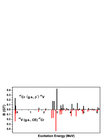
Figure 11: Ground-state GT transition strengths for the $\beta^{+}$-decay of ⁴⁷Cr and the CE reaction of ⁴⁷V. Free axial-vector ($g_{A}=1.26$) are used.

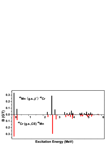
Figure 12: Same as Fig. 11 but for the $A=49$ pair.

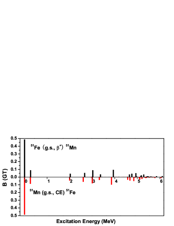
Figure 13: Same as Fig. 11 but for the $A=51$ pair.

Experimentally, B(GT) is accessible through the study of $\beta$-decay and the conjugate charge-exchange (CE) reaction, such as $(p,n)$ reaction. All nuclei discussed above have $\beta^{+}$ decay mode. The distributions of the reduced GT transition strengths for ground-state $\beta^{+}$-decay of ⁴⁷Cr, ⁴⁹Mn, and ⁵¹Fe are plotted in Fig. 11, 12, and 13, respectively. In the lower part of the figures, we give the B(GT) values of conjugate CE processes as a comparison. If isospin symmetry is exactly conserved, the two strength distributions should be identical. The asymmetry deduced from the strengths,

$$\delta^{ISB}=\frac{B(\text{GT;~{}CE})}{B(\text{GT};~{}\beta^{+})}-1,$$ (10)

reflects the ISB effect. Another possible origin of the observed asymmetry come from the non-zero contribution of the induced-tensor term (commonly referred to as second-class current) in Eq. (8). The underlying electroweak theory does not put any limit on the value of $g_{T}$. Investigations for the possible existence of induced-tensor current in weak processes is longstanding Smirnova03 . In the past a few decades, considerable attentions have been paid to light nuclei where large asymmetry has been identified in mirror nuclei GT transitions (See Ref. Smirnova03 for a review). The dominant origin is the strong Coulomb effect which, however, can lead to large uncertainties. One notable property of fp shell nuclei is the relatively small influence from the Coulomb field. More extensive studies concerning the fp nuclei would to very helpful.

Free axial-vector factor with $g_{A}=1.26$ are used in the calculations. For practical applications, a renormalization factor, about 0.744 in $fp$ shell, has to be introduced to account for the quenching effects induced by core-polarization and subnuclear freedoms Caurier05 .

Contributions from orbital and spin terms to M1 transition strengths in $T=1/2$ nuclei can be separated since both isovector M1 and GT decay processes in nuclei are dominated by a $\sigma\tau$-type operator Fujita04 . If isospin symmetry is exact, the final states of the M1 transition and the corresponding GT transition differ only in their $\tau_{z}$ quantum number. Relative strengths between GT and isovector spin-flip M1 strengths can be written as

$$\frac{B(GT^{\pm})}{B(\sigma\tau_{z})}=\frac{8\pi}{3}\left(\frac{g_{A}}{g_{s}^{IS}}\right)^{2}\frac{\langle T_{i},T_{iz},1,\pm 1|T_{f},T_{fz}\rangle^{2}}{\langle T_{i},T_{iz},1,0|T_{f},T_{fz}\rangle^{2}},$$ (11)

by which a more deep insight into the nuclear structure can be deduced. It also has direct astrophysics applications Kawabata04 . Some similar works have been done in $p$ and $sd$ shell, as shown in Ref. Fujita04 . ISB effects on the relation can be evaluated through the calculations of direct overlaps between the analogous final states. We caulcated M1 and GT transitions connecting analogous states in the $T=1/2$ pairs. Theoretical results for B(M1) and B(GT) in mirror pair ⁴⁵Ti and ⁴⁵V are shown in Table 4.

V Summary

$T=1/2$ mirror nuclei in the lower $fp$ shell have been studied by shell-model configuration-mixing calculations based on a microscopic effective Hamiltonian. The effective interaction is derived from the high-precision CD-Bonn NN potential. Calculated level schemes agree well with experimental observations till the $0f_{7/2}$ band termination. The largest discrepancy seen at the $25/2^{-}$ state in ⁴⁹Cr is also discussed. Electromagnetic and Gamow-Teller transition strengths for analogous transitions in the mirror pairs are presented where experimental observations are still insufficient.

The isospin-nonconserving effective interaction enables the investigation of asymmetries existing in nuclear structures and transitions. We calculate ISB contributions to MDE and MED of the mirror pairs. An important role played the term is identified. The discrepancies exist in analogous transitions ara analyzed which can be used to deduce properties of nuclear structures and decay operators.

- (1) A.P. Zuker, S.M. Lenzi, G. Martínez-Pinedo, and A. Poves, Phys. Rev. Lett. 89, 142502 (2002).
- (2) G. Martínez-Pinedo, A.P. Zuker, and E. Caurier, Phys. Rev. C 55, 187 (1997).
- (3) F. Brandolini and C.A. Ur, Phys. Rev. C 71, 054316 (2005).
- (4) A. Poves, J. Sánchez-Solano, E. Caurier, and F. Nowacki, Nucl. Phys. A694 157 (2001).
- (5) M.A. Bentley et al., Phys. Rev. C 73, 024304 (2006); P. Bednarczyk et al., Eur. Phys. J. A20, 45 (2003).
- (6) M.A. Bentley et al., Phys. Lett. B437, 243 (1998).
- (7) D. Tonev et al., Phys. Rev. C 65, 034314 (2002).
- (8) C.D. O’Leary et al., Phys. Rev. Lett. 79, 4349 (1997).
- (9) M.A. Bentley et al., Phys. Rev. C 62, 051303(R) (2000).
- (10) S.J. William et al., Phys. Rev. C 68, 011301(R) (2003).
- (11) S. Shlomo, Rep. Prog. Phys., 41, 66 (1978).
- (12) J.A. Nolen and J.P. Schiffer, Annu. Rev. Nucl. Sci., 19, 491 (1969).
- (13) T. Sukuzi, H. Sagawa, and A. Arima, Nucl. Phys. A536, 141 (1992).
- (14) G.A. Miller, Nucl. Phys. A518, 345 (1990).
- (15) K. Tsushima, K. Saito, and A.W. Thomas, Phys. Lett. B465, 36 (1999).
- (16) R. Machleidt, Phys. Rev. C 63, 024001 (2001).
- (17) B.A. Brown, W.A. Richter, and R. Lindsay, Phys. Lett. B483, 49 (2000).
- (18) H. Müther, A. Polls, and R. Machleidt, Phys. Lett. B445, 259 (1999).
- (19) C. Qi and F.R. Xu, Int. J. Mod. Phys. E15, 1563 (2006); arXiv: nucl-th/0612041.
- (20) T.T.S. Kuo and E. Osnes, Folded-Diagram Theory of Effective Interaction in Nuclei, Atoms and Molecules, Springer Lecture Notes in Physics, Vol. 364 (Springer-Verlag, Berlin, 1990).
- (21) M. Hjorth-Jensen, private commnuication.
- (22) I.S. Towner, A shell model description of light nuclei, (Clarendon Press, Oxford, 1977).
- (23) E. Caurier, G. Martnez-Pinedo, F. Nowacki, A. Poves, and A.P. Zuker, Rev. Mod. Phys. 77, 427 (2005).
- (24) T.T.S. Kuo and G.E. Brown, Nucl. Phys. A114, 241 (1968).
- (25) A. Poves and A.P. Zuker, Phys. Rep. 70, 235 (1981).
- (26) A. Etchegoyen, W.D.M. Rae, N.S. Godwin, W.A. Richter, C.H. Zimmerman, B.A. Brown, W.E. Ormand, and J.S. Winfield, MSU-NSCL Report No. 524 (1985); B.A. Brown, Prog. Part. Nucl. Phys. 47, 517 (2001).
- (27) D.J. Dean, T. Engeland, M. Hjorth-Jensen, M.P. Kartamyshev, and E. Osnes, Prog. Part. Nucl. Phys. 53,419 (2004).
- (28) F. Brandolini et al., Nucl. Phys. A693, 517 (2001).
- (29) A. Bulgac and V.R. Shaginyan, Phys. Lett. B469, 1 (1999).
- (30) W. Oramnd, Phys. Rev. C 55, 2407 (1997).
- (31) J. Ekman et al., Phys. Rev. Lett. 92, 132502 (2004).
- (32) Y. Fujita et al., Phys. Rev. C 70, 054311 (2004), and reference therein.
- (33) N.A. Smirnova and C. Volpe, Nucl. Phys. A714, 441 (2003), and reference therein.
- (34) T. Kawabata et al., Phys. Rev C 70, 034318 (2004).