Abstract

One-parameter exactly separable versions of the X(5) and X(5)-$\beta^{2}$ models, labelled as ES-X(5) and ES-X(5)-$\beta^{2}$ respectively, are derived by using in the Bohr Hamiltonian potentials of the form $u(\beta)+u(\gamma)/\beta^{2}$. Unlike X(5), in these models the $\beta_{1}$ and $\gamma_{1}$ bands are treated on equal footing. Spacings within the $\gamma_{1}$ band are well reproduced by both models, while spacings within the $\beta_{1}$ band are well reproduced only by ES-X(5)-$\beta^{2}$, for which several nuclei with $R_{4/2}=E(4_{1}^{+})/E(2_{1}^{+})$ ratios and [normalized to $E(2_{1}^{+}$)] $\beta_{1}$ and $\gamma_{1}$ bandheads corresponding to the model predictions have been found.

1 Introduction

The introduction of the X(5) critical point symmetry [1] has stirred considerable effort in studying related special solutions [2, 3, 4, 5] of the Bohr collective Hamiltonian [6], as well as in identifying nuclei exhibiting experimentally [7, 8] this behaviour, with considerable success. However, some open questions remain:

1) The separation of variables used in X(5) and related models is approximate. In particular, a potential of the form $u(\beta)+u(\gamma)$ is used, where $\beta$ and $\gamma$ are the usual collective variables [6]. In the X(5) model [1] an infinite square well potential is used as $u(\beta)$, while a harmonic oscillator potential centered around $\gamma=0$ is used as $u(\gamma)$. In the X(5)-$\beta^{2}$ model [5] a harmonic oscillator potential, $\beta^{2}/2$, is used as $u(\beta)$. Separation of variables is based on two approximations: a) the limitation to small angles for $\gamma$, b) the replacement of $\beta^{2}$ by its average value $\langle\beta^{2}\rangle$ in the terms involved in the $\gamma$-equation. Exact numerical diagonalization of the Bohr Hamiltonian [9], carried out using a recently introduced computationally tractable version [10, 11, 12] of the Bohr–Mottelson collective model [6], pointed out that the first approximation is valid for large $\gamma$ stiffness, while the second approximation is valid for small $\gamma$ stiffness.

2) X(5) [1] and the related X(5)-$\beta^{2}$ model [5] contain no free parameter (up to overall scale factors) in the ground state band and $\beta$ bands, but free parameters appear in the $\gamma$ bands and $K=4$ bands. As a result the bandheads of the ground state band and the $\beta$ bands, as well as their internal structure, are fixed by the theory without any free parameter, while the bandheads of the $\gamma$ bands and $K=4$ bands contain free parameters. It would have been preferable to treat the $\beta$ and $\gamma$ bands on equal footing [13].

In the present work we try to circumvent these problems by using potentials of the form $u(\beta)+u(\gamma)/\beta^{2}$, which are known to lead to exact separation of variables [14, 15, 16, 17]. Then the following modifications occur:

1) The second approximation (replacement of $\beta^{2}$ by $\langle\beta^{2}\rangle$) is avoided. The first approximation, namely the limitation to small angles for $\gamma$, is still used, in order to obtain simplified solutions of the $\gamma$ equation, but it can be a good one if stiffness is kept large [9], which indeed turns out to be the case when comparisons to experimental data are performed.

2) The models obtained in this way contain one free parameter in all bands, the stiffness of $\gamma$. As a result the relative position of all bandheads and the internal structure of all bands is fixed by the theory using one parameter, the $\beta_{1}$ and $\gamma_{1}$ bands treated on equal footing, as it is desirable [13].

Recent studies on critical point symmetries [1, 2, 3] have made clear that the relative position of bandheads in a nucleus, as well as the internal spacing in each band, are key structural features which should be reproduced by a model. The internal spacing of the $\beta_{1}$ and $\gamma_{1}$ bands, relative to that of the ground state band, will be shown to provide a stringent test for the various special solutions of the Bohr Hamiltonian.

The models occuring from the exact separation of variables will be described in Section 2, while in Section 3 some numerical results and comparisons to experiment will be given. Finally, a discussion of the present results and plans for further work will be given in Section 4.

2 Spectra

The original Bohr Hamiltonian [6] is

$$H=-{\hbar^{2}\over 2B}\left[{1\over\beta^{4}}{\partial\over\partial\beta}\beta^{4}{\partial\over\partial\beta}+{1\over\beta^{2}\sin 3\gamma}{\partial\over\partial\gamma}\sin 3\gamma{\partial\over\partial\gamma}-{1\over 4\beta^{2}}\sum_{k=1,2,3}{Q_{k}^{2}\over\sin^{2}\left(\gamma-{2\over 3}\pi k\right)}\right]+V(\beta,\gamma),$$ (1)

where $\beta$ and $\gamma$ are the usual collective coordinates, while $Q_{k}$ ($k=1$, 2, 3) are the components of angular momentum in the intrinsic frame, and $B$ is the mass parameter.

One seeks [1] solutions of the relevant Schrödinger equation having the form $\Psi(\beta,\gamma,\theta_{i})=\phi_{K}^{L}(\beta,\gamma){\cal D}_{M,K}^{L}(\theta_{i})$, where $\theta_{i}$ ($i=1$, 2, 3) are the Euler angles, ${\cal D}(\theta_{i})$ denote Wigner functions of them, $L$ are the eigenvalues of angular momentum, while $M$ and $K$ are the eigenvalues of the projections of angular momentum on the laboratory-fixed $z$-axis and the body-fixed $z^{\prime}$-axis respectively.

As pointed out in Ref. [1], in the case in which the potential has a minimum around $\gamma=0$ one can write the angular momentum term of Eq. (1) in the form

$$\sum_{k=1,2,3}{Q_{k}^{2}\over\sin^{2}\left(\gamma-{2\pi\over 3}k\right)}\approx{4\over 3}(Q_{1}^{2}+Q_{2}^{2}+Q_{3}^{2})+Q_{3}^{2}\left({1\over\sin^{2}\gamma}-{4\over 3}\right).$$ (2)

Using this result in the Schrödinger equation corresponding to the Hamiltonian of Eq. (1), introducing [1] reduced energies $\epsilon=2BE/\hbar^{2}$ and reduced potentials $u=2BV/\hbar^{2}$, and assuming that the reduced potential can be separated into two terms of the form $u(\beta,\gamma)=u(\beta)+u(\gamma)/\beta^{2}$, as in Refs. [14, 15, 16, 17], the Schrödinger equation can be separated into two equations

$$\left[-{1\over\beta^{4}}{\partial\over\partial\beta}\beta^{4}{\partial\over\partial\beta}+{L(L+1)\over 3\beta^{2}}+u(\beta)+{\lambda\over\beta^{2}}\right]\xi_{L}(\beta)=\epsilon\xi_{L}(\beta),$$ (3)

$$\left[-{1\over\sin 3\gamma}{\partial\over\partial\gamma}\sin 3\gamma{\partial\over\partial\gamma}+{K^{2}\over 4}\left({1\over\sin^{2}\gamma}-{4\over 3}\right)+u(\gamma)\right]\eta_{K}(\gamma)=\lambda\eta_{K}(\gamma).$$ (4)

Eq. (4) for $\gamma\approx 0$ can be treated as in Ref. [1], considering a potential of the form $u(\gamma)=(3c)^{2}\gamma^{2}/2$ and expanding in powers of $\gamma$. Then Eq. (4) takes the form

$$\left[-{1\over\gamma}{\partial\over\partial\gamma}\gamma{\partial\over\partial\gamma}+{K^{2}\over 4\gamma^{2}}+(3c)^{2}{\gamma^{2}\over 2}\right]\eta_{K}(\gamma)=\epsilon_{\gamma}\eta_{K}(\gamma),$$ (5)

with $\epsilon_{\gamma}=\lambda+{K^{2}\over 3}$. The solution is given in terms of Laguerre polynomials [1]

$$\epsilon_{\gamma}=(3c)(n_{\gamma}+1),\qquad n_{\gamma}=0,1,2,\ldots,$$ (6)

$$n_{\gamma}=0,\quad K=0;\qquad n_{\gamma}=1,\quad K=\pm 2;\qquad n_{\gamma}=2,\quad K=0,\pm 4;\qquad\ldots,$$ (7)

$$\eta_{n_{\gamma},K}(\gamma)=C_{n,K}\gamma^{|K/2|}e^{-(3c)\gamma^{2}/2}L_{n}^{|K/2|}(3c\gamma^{2}),\qquad n=(n_{\gamma}-|K/2|)/2.$$ (8)

Eq. (3) is then solved exactly for the case in which $u(\beta)$ is an infinite well potential

$$u(\beta)=\left\{\begin{array}[]{ll}0&\mbox{if $\beta\leq\beta_{W}$}\\ \infty&\mbox{for $\beta>\beta_{W}$}\end{array}\right..$$ (9)

Setting [1] $\tilde{\xi}(\beta)=\beta^{3/2}\xi(\beta)$, $\epsilon=k_{\beta}^{2}$, and $z=\beta k_{\beta}$, one obtains the Bessel equation

$${d^{2}\tilde{\xi}\over dz^{2}}+{1\over z}{d\tilde{\xi}\over dz}+\left[1-{\nu^{2}\over z^{2}}\right]\tilde{\xi}=0,$$ (10)

with

$$\nu=\sqrt{{L(L+1)-K^{2}\over 3}+{9\over 4}+3c(n_{\gamma}+1)}.$$ (11)

From the boundary condition $\tilde{\xi}(\beta_{W})=0$ the energy eigenvalues are then [1]

$$\epsilon_{\beta;s,L}=(k_{s,L})^{2},\qquad k_{s,L}={x_{s,L}\over\beta_{W}},$$ (12)

where $x_{s,L}$ is the $s$-th zero of the Bessel function $J_{\nu}(k_{s,L}\beta)$, while the relevant eigenfunctions are

$$\xi_{s,L}(\beta)=C_{s,L}\beta^{-3/2}J_{\nu}(k_{s,L}\beta),$$ (13)

where $C_{s,L}$ are normalization constants. For $K=0$ one has $L=0$, 2, 4, …, while for $K\neq 0$ one obtains $L=K$, $K+1$, $K+2$, …

The full wave function reads

$$\Psi(\beta,\gamma,\theta_{i})=C_{s,L}\beta^{-3/2}J_{\nu}(k_{s,L}\beta)\eta_{n_{\gamma},K}(\gamma){\cal D}^{L}_{MK}(\theta_{i}),$$ (14)

and should be properly symmetrized [1]

$$\Psi(\beta,\gamma,\theta_{i})={1\over\sqrt{2}}\left[\phi_{L,K}(\beta,\gamma){\cal D}^{L}_{MK}(\theta_{i})+(-1)^{L+K}\phi_{L,-K}{\cal D}^{L}_{M,-K}(\theta_{i})\right].$$ (15)

Bands occuring in this model, characterized by ($s$, $n_{\gamma}$), include the ground state band $(1,0)$, the $\beta_{1}$-band $(2,0)$, the $\gamma_{1}$-band $(1,1)$, the first $K=4$ band $(1,2)$. The relative position of all levels depends on the single parameter $c$. Therefore the main difference between the present model and X(5) is that in the present model all bands are fixed by the single parameter $c$, while in X(5) the ground state band and the other $n_{\gamma}=0$ bands are fixed in a parameter-free way, but the bandheads of the $n_{\gamma}\neq 0$ bands depend on free parameters.

In Ref. [18] a variant of the X(5) model has been considered, in which during the separation of variables the term $K^{2}/3$ has been kept in the $\beta$-equation, while in Ref. [1] this term has been put in the $\gamma$-equation. This choice leads to different results (different expression for $\nu$, in particular) when the method of Refs. [1, 18] is followed, but it makes no difference in the present approach.

Eq. (3) is exactly soluble also in the case in which $u(\beta)=\beta^{2}/2$. In this case, which is analogous to the X(5)-$\beta^{2}$ model [5], the eigenfunctions are [19]

$$F_{n}^{L}(\beta)=\left[{2n!\over\Gamma\left(n+a+{5\over 2}\right)}\right]^{1/2}\beta^{a}L_{n}^{a+{3\over 2}}(\beta^{2})e^{-\beta^{2}/2},$$ (16)

where $\Gamma(n)$ stands for the $\Gamma$-function, $L_{n}^{a}(z)$ denotes the Laguerre polynomials, and

$$a=-{3\over 2}+\sqrt{{L(L+1)-K^{2}\over 3}+{9\over 4}+3c(n_{\gamma}+1)},$$ (17)

while the energy eigenvalues are

$$E_{n,L}=2n+a+{5\over 2}=2n+1+\sqrt{{L(L+1)-K^{2}\over 3}+{9\over 4}+3c(n_{\gamma}+1)},\qquad n=0,1,2,\ldots$$ (18)

In the above, $n$ is the usual oscillator quantum number. A formal correspondence between the energy levels of the X(5) analogue and the present X(5)-$\beta^{2}$ analogue can be established through the relation

$$n=s-1.$$ (19)

It should be remembered, however, that the origin of the two quantum numbers is different, $s$ labelling the order of a zero of a Bessel function and $n$ labelling the number of zeros of a Laguerre polynomial. In the present notation, the ground state band corresponds to $s=1$ ($n=0$). For the energy states the notation $E_{s,L}=E_{n+1,L}$ of Ref. [1] will be kept.

On the present approach the following general comments apply.

a) The use of a potential of the form $u(\beta)+u(\gamma)/\beta^{2}$, instead of a potential of the form $u(\beta)+u(\gamma)$ [as in X(5) and X(5)-$\beta^{2}$] leads to exact separation of variables instead of an approximate one [14, 15, 16, 17]. As a result, no $\beta^{2}$ factors appear in the $\gamma$-equation, and therefore the approximation of replacing $\beta^{2}$ by its average value, $\langle\beta^{2}\rangle$, used in X(5) and X(5)-$\beta^{2}$, is avoided. Exact numerical diagonalizations [9] of the Bohr Hamiltonian have demonstrated that this approximation is valid only for small $\gamma$ stiffness. This requirement is removed in the present case.

b) However, the treatment of the $\gamma$-equation in the present approach is based on the same approximation of small $\gamma$ angles also used in the X(5) and X(5)-$\beta^{2}$ models. The potential $(3c)^{2}\gamma^{2}/2$ used here is the lowest order approximation for small $\gamma$ to the potential $c^{2}(1-\cos 3\gamma)$, which has also been used in Ref. [20]. It should be reminded that the dependence on $\cos 3\gamma$ results from the symmetry requirements [6] of the Bohr Hamiltonian, explicitly listed in Ref. [21]. A two-dimensional oscillator in $\gamma$, similar to the one obtained here, has also been obtained in Ref. [20] in the limit of large $\gamma$ stiffness (large $c$ in the present notation). The exact numerical diagonalizations of the Bohr Hamiltonian carried out in Ref. [9] consistently demonstrated that the small angle approximation for $\gamma$ is good for large $\gamma$ stiffness, which in the present models can be achieved, since the requirement of small $\gamma$ stiffness is not present any more, as discussed in point a). In Sec. 3 we shall see that experimental data are reproduced for values of $c$ of order 10, corresponding to $(3c)^{2}\approx 900$.

c) Small oscillations in $\gamma$ around the zero value, corresponding to axially deformed prolate shapes, have also been considered in Ref. [22], leading to the conclusion that $K$ can be considered as a good quantum number either if $\gamma$ is fixed to zero, or if the nucleus is strongly deformed. In Sec. 3 we shall see that good agreement with experimental data is obtained for nuclei with $R_{4/2}=E(4_{1}^{+})/E(2_{1}^{+})>3.15$, i.e. for nuclei which are well deformed.

3 Numerical results and comparison to experiment

Numerical results for the present models, referred to as exactly separable X(5) [ES-X(5)] and exactly separable X(5)-$\beta^{2}$ [ES-X(5)-$\beta^{2}$] respectively, are shown in Table 1, together with results for several other models, including X(5) [1], exact numerical diagonalization of the Bohr Hamiltonian [9] (labelled by “Caprio”), X(5)-$\beta^{2n}$ ($n=1,2,3,4$) [5], X(5) with a Davidson potential

$$u(\beta)=\beta^{2}+{\beta_{0}^{4}\over\beta^{2}},$$ (20)

where $\beta_{0}$ is the minimum of the potential [4], labelled as X(5)-D. The collective quantities reported in Table 1 include the ground state band ratio $R_{4/2}=E(4_{1}^{+})/E(2_{1}^{+})$, the bandheads of the $\beta_{1}$ and $\gamma_{1}$ bands, $E(0_{\beta}^{+})$ and $E(2_{\gamma}^{+})$, normalized to $E(2_{1}^{+})$, the spacings within the $\beta_{1}$ band relative to these of the ground state band

$$R_{2,0,\beta,g}={E(2_{\beta}^{+})-E(0_{\beta}^{+})\over E(2_{1}^{+})},\qquad R_{4,2,\beta,g}={E(4_{\beta}^{+})-E(2_{\beta}^{+})\over E(4_{1}^{+})-E(2_{1}^{+})},$$ (21)

and the spacing within the $\gamma_{1}$ band relative to that of the ground state band

$$R_{4,2,\gamma,g}={E(4_{\gamma}^{+})-E(2_{\gamma}^{+})\over E(4_{1}^{+})-E(2_{1}^{+})}.$$ (22)

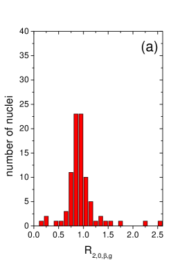
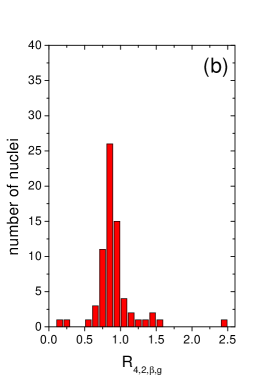
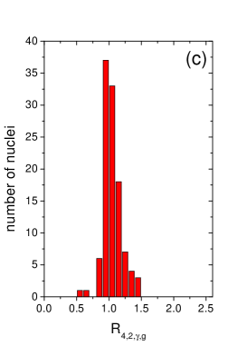
Figure 1: Experimental data for the energy ratios $R_{2,0,\beta,g}$ [Eq. (21)] (a), $R_{4,2,\beta,g}$ [Eq. (21)] (b), and $R_{4,2,\gamma,g}$ [Eq. (22)] (c). For each ratio, all nuclei with $A>50$ (excluding magic and semimagic nuclei) for which sufficient experimental data (taken from Ref. [23]) exist, have been taken into account.

Experimental values for the energy ratios $R_{2,0,\beta,g}$, $R_{4,2,\beta,g}$, and $R_{4,2,\gamma,g}$ are shown in Fig. 1 for all nuclei with $A>50$ (excluding magic and semimagic nuclei). The following comments can be made:

1) From Fig. 1(a),(b) it is clear that the majority of nuclei exhibit ratios $R_{2,0,\beta,g}$ and $R_{4,2,\beta,g}$ close to 1 or slightly below it, indicating that the spacings within the $\beta_{1}$ band are similar to the spacings within the ground state band, as expected for a band displaced from the ground state band by one quantum of $\beta$ vibration. Ratios exactly equal to 1 are provided by the X(5)-$\beta^{2}$, ES-X(5)-$\beta^{2}$, and X(5)-D models, guaranteed by the $\beta^{2}$ term present in the relevant potentials. X(5) gives values of 1.8 and 1.7 respectively, the well known point of disagreement with experimental ratios by a factor close to 2 [7, 8]. The exact numerical diagonalization of Ref. [9] provides similar or higher values, while ES-X(5) gives values around 1.5 . The X(5)-$\beta^{4}$, X(5)-$\beta^{6}$, and X(5)-$\beta^{8}$ models interpolate between X(5)-$\beta^{2}$ and X(5), as expected, since higher powers of $\beta^{2n}$ closer approximate the infinite well potential.

2) The above observations can be understood in the following way. It is known that the problem of overprediction of the spacing within the $\beta_{1}$ band by X(5) can be resolved by replacing the infinite well potential in $\beta$ by a potential with sloped walls [2]. The combination of the five-dimensional centrifugal term with the sloped well provides a potential with a minimum, resembling the Davidson potential of Eq. (20) as well as the sum of a harmonic oscillator potential and a centrifugal term.

3) From Fig. 1(c) it is clear that the majority of nuclei exhibit ratios $R_{4,2,\gamma,g}$ close to 1, indicating that the spacings within the $\gamma_{1}$ band are similar to the spacings within the ground state band. Among the models of Table 1, X(5), X(5)-$\beta^{2n}$, as well as X(5)-D, provide values slightly higher than 1, the ES-X(5) and ES-X(5)-$\beta^{2}$ models give values slightly lower than 1, while the exact numerical diagonalization of Ref. [9] is in between. It is interesting that in the X(5)-D model for large parameter values, the spacing within the $\gamma_{1}$ band becomes the same as within the ground state band and the $\beta_{1}$ bands, as expected in the SU(3) limit.

From the above observations it is expected that the one-parameter ES-X(5)-$\beta^{2}$ and X(5)-D models, as well as X(5)-$\beta^{2}$, are more appropriate for reproducing the correct spacings within the $\beta_{1}$ and $\gamma_{1}$ bands. However, the position of the bandheads is also important. It is then reasonable to look for nuclei for which a model can closely reproduce the $R_{4/2}$ ratio, characterizing the development of the ground state band, but also the development of the $\beta_{1}$ and $\gamma_{1}$ bands, according to the systematics of Fig. 1, as well as the normalized bandheads $E(0_{\beta}^{+})/E(2_{1}^{+})$ and $E(2_{\gamma}^{+})/E(2_{1}^{+})$. A search of all even nuclei with $Z>50$, for which sufficient data exist [23], provided the results shown in Table 2. 18 examples have been found for ES-X(5)-$\beta^{2}$, as well as 4 examples for ES-X(5).

The basic difference between ES-X(5)-$\beta^{2}$ and ES-X(5) is shown in Table 3, where the ground state, $\beta_{1}$ and $\gamma_{1}$ bands of ¹⁵⁶Gd, a good example of ES-X(5)-$\beta^{2}$, and ¹⁶²Dy, a good example of ES-X(5), are shown. In the first case the agreement between theory and experiment remains good in all three bands up to high angular momenta, while in the second case this holds only for the ground state and $\gamma_{1}$ bands, the theoretical $\beta_{1}$ band diverging from the data with increasing angular momentum.

A final remark concerning the physical content of the models developed here, based on the potential of the form $u(\beta)+u(\gamma)/\beta^{2}$ [14, 15, 16, 17]. As already remarked in Ref. [14], one expects $\gamma$ stability to increase with deformation. This is corroborated by the results shown in Table 2, where it is clear that $c$ is increasing with $R_{4/2}$, indicating that $u(\gamma)$ is becoming more and more steep with increasing deformation, restricting the nucleus to $\gamma$ values very close to zero. As a result, the present models are applicable to strongly deformed nuclei close to axial symmetry.

4 Discussion

In summary, exactly separable one-parameter versions of the X(5) and X(5)-$\beta^{2}$ models, labelled as ES-X(5) and ES-X(5)-$\beta^{2}$, have been derived, by using potentials of the form $u(\beta)+u(\gamma)/\beta^{2}$. Unlike X(5), in these models the $\beta_{1}$ and $\gamma_{1}$ bands are treated on equal footing. The spacings within the $\gamma_{1}$ band are in agreement to experimental evidence in both models, while the spacings within the $\beta_{1}$ band are reproduced correctly only by ES-X(5)-$\beta^{2}$. Several nuclei for which the $R_{4/2}$ ratio, as well as the normalized positions of the $\beta_{1}$ and $\gamma_{1}$ bandheads are closely reproduced by ES-X(5)-$\beta^{2}$ have been identified. A detailed study of the complete level schemes of these nuclei, including B(E2) transition rates, is deferred to a longer publication.

Table 1: The key collective quantities $R_{4/2}=E(4_{1}^{+})/E(2_{1}^{+})$, normalized $\beta_{1}$ bandhead $E(0_{\beta}^{+})/E(2_{1}^{+})$ (labelled as $0_{\beta}^{+}/2_{1}^{+}$), normalized $\gamma_{1}$ bandhead $E(2_{\gamma}^{+})/E(2_{1}^{+})$ (labelled as $2_{\gamma}^{+}/2_{1}^{+}$), spacings of the $\beta_{1}$ band relative to the ground state band $R_{2,0,\beta,g}$ [Eq. (21)] and $R_{4,2,\beta,g}$ [Eq. (21)], as well as spacing of the $\gamma_{1}$ band relative to the ground state band $R_{4,2\gamma,g}$ [Eq. (22)] are listed for different models, including X(5)-$\beta^{2n}$ [5], X(5) [1], X(5)-D [4], Caprio’s exact numerical diagonalization of the Bohr Hamiltonian [9], and the present exactly separable analogues of X(5) [ES-X(5)] and X(5)-$\beta^{2}$ [ES-X(5)-$\beta^{2}$]. Parameter values, if present, are listed in the column “Par”, using the definition and symbol of the relevant original publication. The notation “par” indicates that the corresponding quantity depends on an additional free parameter.

model	Par	$R_{4/2}$	$0_{\beta}^{+}/2_{1}^{+}$	$2_{\gamma}^{+}/2_{1}^{+}$	$R_{2,0,\beta,g}$	$R_{4,2,\beta,g}$	$R_{4,2,\gamma,g}$
X(5)-$\beta^{2}$		2.646	3.562	par	1.000	1.000	1.132
X(5)-$\beta^{4}$		2.769	4.352	par	1.250	1.205	1.101
X(5)-$\beta^{6}$		2.824	4.816	par	1.416	1.344	1.089
X(5)-$\beta^{8}$		2.852	5.091	par	1.528	1.441	1.083
X(5)		2.904	5.649	par	1.801	1.701	1.071
X(5)-D	$\beta_{0}$
	0.0	2.646	3.562	par	1.000	1.000	1.131
	1.0	2.756	4.094	par	1.000	1.000	1.108
	1.5	2.978	5.756	par	1.000	1.000	1.064
	2.0	3.156	8.772	par	1.000	1.000	1.031
	5.0	3.327	50.130	par	1.000	1.000	1.001
Caprio	a
	0.	2.20	3.03	2.20	1.77	0.31	1.16
	200.	2.76	5.66	6.09	2.31	1.74	1.15
	400.	3.02	8.37	10.12	2.19	1.76	1.04
	600.	3.12	10.26	13.42	2.00	1.79	0.95
	800.	3.17	11.71	16.19	1.91	1.70	1.00
	1000.	3.20	12.89	18.66	1.84	1.69	0.97
ES-X(5)	c
	2.0	3.166	10.298	3.166	1.649	1.606	0.929
	4.0	3.234	13.643	5.955	1.579	1.552	0.909
	6.0	3.264	16.451	8.764	1.534	1.515	0.904
	8.3	3.283	19.292	12.013	1.497	1.484	0.903
	10.0	3.292	21.210	14.423	1.477	1.465	0.904
	12.0	3.299	23.317	17.266	1.456	1.447	0.905
	13.7	3.304	25.012	19.692	1.442	1.433	0.906
ES-X(5)-$\beta^{2}$	c
	2.0	3.006	6.074	3.006	1.000	1.000	0.852
	4.0	3.117	7.806	5.516	1.000	1.000	0.796
	6.0	3.171	9.217	8.011	1.000	1.000	0.771
	8.0	3.204	10.439	10.502	1.000	1.000	0.757
	10.0	3.225	11.531	12.991	1.000	1.000	0.749
	12.0	3.241	12.529	15.478	1.000	1.000	0.742
	14.0	3.252	13.453	17.965	1.000	1.000	0.738

Table 2: Comparison of theoretical predictions of the exactly separable analogue of the X(5)-$\beta^{2}$ model [ES-X(5)-$\beta^{2}$] (upper part) and of the exactly separable analogue of the X(5) model [ES-X(5)] (lower part) to experimental $R_{4/2}=E(4_{1}^{+})/E(2_{1}^{+})$ ratios, as well as to experimental $\beta_{1}$ and $\gamma_{1}$ bandheads, normalized to the $2_{1}^{+}$ state and labelled by $0_{\beta}^{+}/2_{1}^{+}$ and $2_{\gamma}^{+}/2_{1}^{+}$ respectively. All data have been taken from Ref. [23].

nucleus	$R_{4/2}$	$0_{\beta}^{+}/2_{1}^{+}$	$2_{\gamma}^{+}/2_{1}^{+}$	$c$	$R_{4/2}$	$0_{\beta}^{+}/2_{1}^{+}$	$2_{\gamma}^{+}/2_{1}^{+}$
	exp	exp	exp		th	th	th
188Os	3.083	7.008	4.083	2.9	3.068	6.908	4.139
186Os	3.165	7.736	5.596	4.0	3.117	7.806	5.516
184Os	3.203	8.698	7.870	5.7	3.165	9.019	7.637
184W	3.274	9.014	8.122	6.0	3.171	9.217	8.011
162Er	3.230	10.654	8.827	7.0	3.189	9.847	9.257
166Yb	3.228	10.189	9.108	7.0	3.189	9.847	9.257
158Dy	3.206	10.014	9.567	7.3	3.194	10.028	9.630
170Er	3.310	11.335	11.883	9.2	3.218	11.107	11.995
182W	3.291	11.346	12.201	9.4	3.220	11.215	12.244
180Hf	3.307	11.807	12.855	10.0	3.225	11.531	12.991
156Gd	3.239	11.796	12.972	10.0	3.225	11.531	12.991
228Ra	3.207	11.300	13.258	10.1	3.226	11.583	13.115
170Yb	3.293	12.692	13.598	10.7	3.231	11.890	13.861
230Th	3.273	11.934	14.687	11.3	3.236	12.189	14.608
228Th	3.235	14.402	16.776	13.4	3.249	13.182	17.219
154Sm	3.254	13.410	17.567	13.7	3.251	13.318	17.592
172Yb	3.305	13.245	18.616	14.4	3.254	13.630	18.463
232U	3.291	14.530	18.221	14.5	3.255	13.674	18.587
166Er	3.289	18.118	9.754	6.7	3.271	17.352	9.751
162Dy	3.294	17.332	11.011	7.6	3.278	18.462	11.022
162Gd	3.291	19.792	11.983	8.3	3.283	19.292	12.013
176Yb	3.308	21.661	15.352	10.6	3.294	21.857	15.275

Table 3: Comparison of the predictions of the exactly separable analogue of the X(5)-$\beta^{2}$ model [ES-X(5)-$\beta^{2}$] (with $c=10.0$) to the experimental spectrum of ¹⁵⁶Gd [23] (upper part), and of the predictions of the exactly separable analogue of X(5) [ES-X(5)] (with $c=7.6$) to the experimental spectrum of ¹⁶²Dy [23] (lower part). The energy levels of the ground state band (gsb), the $\beta_{1}$ band, and the $\gamma_{1}$ band are normalized to the $2_{1}^{+}$ level.

		gsb	gsb	$\beta_{1}$	$\beta_{1}$		$\gamma_{1}$	$\gamma_{1}$
	L	exp	th	exp	th	L	exp	th
156Gd
	0	0.000	0.000	11.796	11.531	2	12.972	12.991
	2	1.000	1.000	12.695	12.531	3	14.027	13.712
	4	3.239	3.225	14.587	14.757	4	15.235	14.656
	6	6.573	6.468	17.311	17.999	5	16.937	15.811
	8	10.848	10.500	20.775	22.031	6	18.474	17.162
	10	15.916	15.122	24.952	26.653	7	20.792	18.692
	12	21.631	20.179	30.435	31.710	8	22.607	20.388
	14	27.828	25.559			9	25.285	22.233
	16	34.388	31.180			10	27.452	24.213
162Dy
	0	0.000	0.000	17.332	18.462	2	11.011	11.022
	2	1.000	1.000	18.020	19.969	3	11.938	11.909
	4	3.294	3.278	19.518	23.369	4	13.154	13.081
	6	6.800	6.733	21.913	28.445	5	14.664	14.532
	8	11.412	11.259	24.619	34.975	6	16.420	16.255
	10	17.044	16.768	28.041	42.778	7	18.477	18.242
	12	23.572	23.195	32.156	51.721	8	20.709	20.485
	14	30.895	30.493	36.640	61.705	9	23.284	22.975
	16	38.904	38.625			10	25.879	25.708
	18	47.583	47.568			11	28.981	28.676
						12	31.396	31.873
						13	35.453	35.295
						14	39.437	38.936

Figures

References

- [1] F. Iachello, Phys. Rev. Lett. 87 (2001) 052502.
- [2] M. A. Caprio, Phys. Rev. C 69 (2004) 044307.
- [3] N. Pietralla, O. M. Gorbachenko, Phys. Rev. C 70 (2004) 011304.
- [4] D. Bonatsos, D. Lenis, N. Minkov, D. Petrellis, P. P. Raychev, P. A. Terziev, Phys. Lett. B 584 (2004) 40.
- [5] D. Bonatsos, D. Lenis, N. Minkov, P. P. Raychev, P. A. Terziev, Phys. Rev. C 69 (2004) 014302.
- [6] A. Bohr, Mat. Fys. Medd. K. Dan. Vidensk. Selsk. 26 (1952) no. 14.
- [7] R. F. Casten, N. V. Zamfir, Phys. Rev. Lett. 87 (2001) 052503.
- [8] R. Krücken, et al., Phys. Rev. Lett. 88 (2002) 232501.
- [9] M. A. Caprio, Phys. Rev. C 72 (2005) 054323.
- [10] D. J. Rowe, Nucl. Phys. A 735 (2004) 372.
- [11] D. J. Rowe, P. S. Turner, J. Repka, J. Math. Phys. 45 (2004) 2761.
- [12] D. J. Rowe, P. S. Turner, Nucl. Phys. A 753 (2005) 94.
- [13] F. Iachello, in G. Lo Bianco (Ed.), Symmetries and Low-Energy Phase Transition in Nuclear-Structure Physics, U. Camerino (2006) 1.
- [14] L. Wilets and M. Jean, Phys. Rev. 102, 788 (1956).
- [15] L. Fortunato, Eur. Phys. J. A 26, s01 (2005) 1.
- [16] L. Fortunato, Phys. Rev. C 70 (2004) 011302.
- [17] L. Fortunato, S. De Baerdemacker, and K. Heyde, Phys. Rev. C 74, 014310 (2006).
- [18] R. Bijker, R. F. Casten, N. V. Zamfir, E. A. McCutchan, Phys. Rev. C 68 (2003) 064304.
- [19] M. Moshinsky, J. Math. Phys. 25 (1984) 1555.
- [20] M. Jean, Nucl. Phys. 21 (1960) 142.
- [21] T. M. Corrigan, F. J. Margetan, S. A. Williams, Phys. Rev. C 14 (1976) 2279.
- [22] A. S. Davydov, Nucl. Phys. 24 (1961) 682.
- [23] Nuclear Data Sheets, as of December 2005.