Predictions for two-pion correlations for $\sqrt{s}=14$ TeV proton-proton collisions

Abstract

A simple model based on relativistic geometry and final-state hadronic rescattering is used to predict pion source parameters extracted in two-pion correlation studies of proton-proton collisions at $\sqrt{s}=14$ TeV. By comparing the results of these model studies with data, it might be possible to obtain information on the hadronization time in these collisions. As a test of this model, comparisons between existing two-pion correlation data at $\sqrt{s}=1.8$ TeV and results from the model are made. It is found at this lower energy that using a short hadronization time in the model best describes the trends of the data.

I Introduction

With first proton-proton collisions at $\sqrt{s}=14$ TeV from the Large Hadron Collider (LHC) being only about a year (or so) away, it is tempting to use simple models to make baseline predictions of what we might expect for ”bread and butter” observables at this unexplored energy. Comparisons between data and such models could give us a first impression of the presence of new physics which might cause significant disagreements between them. If significant disagreements are seen, the simple models might then be used to point in a direction as to the nature of the new physics.

The ”bread and butter” observable studied in the present work is two-pion correlations. From this observable, information about the space-time geometry of the pion emissions produced in the proton-proton collisions can be, at least in principle, extracted using the interferometric technique pioneered by Hanbury Brown and Twiss (HBT) hbt1 and first used in particle physics in $p-\bar{p}$ collisions by Goldhaber, Goldhaber, Lee and Pais (GGLP) gglp . Many such experimental studies using this technique have been carried out over the past nearly 50 years Lisa:2005a ; Humanic:2006a , the highest energy study being carried out at the Tevatron with $p-\bar{p}$ collisions at $\sqrt{s}=1.8$ TeV e735 . The strategy of the present study is to use a simple model based on relativistic geometry and final-state hadronic rescattering to predict pion source parameters extracted in two-pion correlation studies of proton-proton collisions at $\sqrt{s}=14$ TeV. As a test of this model, comparisons with existing two-pion correlation data at $\sqrt{s}=1.8$ TeV are made. A similar study which served as the inspiration for the present work has been published by Paic and Skowronski Paic:2005a . The main differences between that study and the present approach are that in the present approach 1) a somewhat simpler geometric picture of hadronization is used, e.g. no explicit identification of jets vs. non-jets is made, 2) for simplicity only 1-dimensional invariant correlation functions are studied, 3) at Tevatron energy Gaussian fits to the model-generated two-pion correlation functions are made to directly compare with experiment whereas at LHC energy the two-pion correlation function is fit to a more general function , and 4) the effects of final-state hadronic rescattering are included since particle multiplicities become relatively large at these higher energies.

The paper is divided into the following sections: Section II gives a description of the model, Section III presents results of the model and discussions for $p-p$ collisions at $\sqrt{s}=14$ TeV and $p-\bar{p}$ at 1.8 TeV and comparisons with Tevatron data, and Section IV gives conclusions and summary.

II Description of the model

The model calculations are carried out in four main steps: A) generate hadrons in $p-p$ and $p-\bar{p}$ collisions from PYTHIA pythia6.3 , B) employ a simple space-time geometry picture for hadronization of the PYTHIA-generated hadrons, C) calculate the effects of final-state rescattering among the hadrons, and D) impose Bose-Einstein correlations pairwise on pions, calculate correlation functions, and fit the correlation functions with Gaussian or more general functions to extract pion source parameters. These steps will now be discussed in more detail.

II.1 Generation of the $p-p$ collisions with PYTHIA

The $p-p$ and $p-\bar{p}$ collisions were modeled with the PYTHIA code pythia6.3 , version 6.326. The parton distribution functions used were the same as used in Ref. bh . Events were generated in “minimum bias” mode, i.e. setting the low-$p_{T}$ cutoff for parton-parton collisions to zero (or in terms of the actual PYTHIA parameter, $ckin(3)=0$). Runs were made both with $\sqrt{s}=$ 1.8 and 14 TeV to simulate Tevatron and LHC (full energy) collisions, respectively. Information saved from a PYTHIA run for use in the next step of the procedure were the momenta and identities of the “direct” (i.e. redundancies removed) hadrons (all charge states) $\pi$, $K$, $p$, $n$, $\Lambda$, $\rho$, $\omega$, $\eta$, ${\eta}^{\prime}$, $\phi$, and $K^{*}$. These particles were chosen since they are the most common hadrons produced and thus should have the biggest effect on the two-pion correlation functions extracted in these calculations.

II.2 The space-time geometry picture for hadronization

The simple space-time geometry picture for hadronization consists of the emission of a PYTHIA particle from a thin uniform disk of radius 1 fm in the plane transverse (x-y) to the beam direction (z) followed by its hadronization which occurs in the proper time of the particle, $\tau$. The space-time coordinates at hadronization in the lab frame $(x_{h},y_{h},z_{h},t_{h})$ for a particle with momentum coordinates $(p_{x},p_{y},p_{z})$, energy $E$, rest mass $m_{0}$, and transverse disk coordinates $(x_{0},y_{0})$ can then be written as

$$x_{h}=x_{0}+\tau\frac{p_{x}}{m_{0}}$$ (1)

$$y_{h}=y_{0}+\tau\frac{p_{y}}{m_{0}}$$ (2)

$$z_{h}=\tau\frac{p_{z}}{m_{0}}$$ (3)

$$t_{h}=\tau\frac{E}{m_{0}}$$ (4)

The simplicity of this geometric picture is now clear: it is just an expression of causality with the assumption that all particles hadronize with the same proper time, $\tau$. A similar hadronization picture (with an initial point source) has been applied to $e^{+}-e^{-}$ collisionscsorgo . We do not a priori know the value of $\tau$ but from the geometric scale of a $p-p$ collision we might guess that $\tau$ falls in the range $0<\tau<\sim 1$ fm/c. In order to study the dependence of the results of the model on this parameter, calculations will be carried out with a range of values. Note that the HBT results given later from the model are found to not strongly depend on the choice of the radius of the initial transverse disk within a range of $1\pm 0.5$ fm or on the choice of a disk versus a smoothly dropping off distribution such as a Gaussian due to the effects of these assumptions being “washed out” by the randomizing effects of the “causality term” in Eqs.(1) and (2) and of final-state rescattering.

II.3 Final-state hadronic rescattering

Since very high energy $p-p$ collisions are being considered here and the most interesting collisions are normally those producing the highest particle multiplicities, it seems possible that at early times during the collision the particle density could reach a level at which significant final-state hadronic rescattering might take place. An attempt is made to take this effect into account in the present calculations.

The hadronic rescattering calculational method used is similar to that employed in previous calculations for heavy-ion collisions at CERN Super Proton Synchrotron (SPS) energies and BNL Relativistic Heavy Ion Collider (RHIC) energies Humanic:1998a ; Humanic:2006a , where particle densities are high enough to produce significant rescattering effects. Rescattering is simulated with a semi-classical Monte Carlo calculation which assumes strong binary collisions between hadrons. Relativistic kinematics is used throughout. The hadrons input into the calculation from PYTHIA are pions, kaons, nucleons and lambdas ($\pi$, K, N, and $\Lambda$), and the $\rho$, $\omega$, $\eta$, ${\eta}^{\prime}$, $\phi$, $\Delta$, and $K^{*}$ resonances. For simplicity, the calculation is isospin averaged (e.g. no distinction is made among a $\pi^{+}$, $\pi^{0}$, and $\pi^{-}$).

The rescattering calculation finishes with the freeze out and decay of all particles. Starting from the initial stage ($t=0$ fm/c), the positions of all particles in each event are allowed to evolve in time in small time steps ($\Delta t=0.1$ fm/c) according to their initial momenta. At each time step each particle is checked to see a) if it has hadronized ($t>t_{h}$, where $t_{h}$ is given in Equation 4.), b) if it decays, and c) if it is sufficiently close to another particle to scatter with it. Isospin-averaged s-wave and p-wave cross sections for meson scattering are obtained from Prakash et al.Prakash:1993a and other cross sections are estimated from fits to hadron scattering data in the Review of Particle Physicspdg . Both elastic and inelastic collisions are included. The calculation is carried out to 20 fm/c which allows enough time for the rescattering to finish (as a test, calculations were also carried out to 40 fm/c with no changes in the results). Note that when this cutoff time is reached, all un-decayed resonances are allowed to decay with their natural lifetimes and their projected decay positions and times are recorded. The rescattering calculation is described in more detail elsewhere Humanic:2006a ; Humanic:1998a . The validity of the numerical methods used in the rescattering code have recently been studied and verifiedHumanic:2006b .

II.4 Correlation function calculation and fitting

For the two-pion correlation calculations, the two-pion correlation function is formed and either a Gaussian or more general function is fitted to it to extract the final fit parameters. In the present calculation boson statistics are introduced after rescattering using a method of pair-wise symmetrization of bosons in a plane-wave approximation Humanic:1986a . The final step in the calculation is extracting fit parameters by fitting a parameterization to the Monte- Carlo-produced two-pion invariant correlation function, $C(Q_{inv})$, where $Q_{inv}$ is the invariant momentum difference defined as the magnitude of the difference between the four-momenta of the two pions, i.e. $Q_{inv}=\mid p_{1}-p_{2}\mid$. The forms of the Gaussian and general fit functions are given, respectively, by

$$C(Q_{inv})=A[1+\lambda\exp(-R^{2}Q_{inv}^{2})]$$ (5)

or,

$$C(Q_{inv})=A[1+\lambda\cos{(\alpha Q_{inv}^{2})}\exp(-R^{\delta}Q_{inv}^{\delta})]$$ (6)

where $R$ is a radius parameter, $\lambda$ is an empirical parameter normally employed to help fit the function to the correlation function (i.e. $\lambda=1$ in the ideal case of pure Bose-Einstein correlations), $\alpha$ describes oscillations in the correlation function, $\delta$ represents the degree to which the correlation function falls off with increasing $Q_{inv}$, and $A$ is a normalization factor. For the Gaussian case, a simple connection can be made between $R$ and the space-time distribution of the pion source, $\rho(r)$, where $r$ is a position variable, via

$$\rho(r)\sim\exp(-\frac{r^{2}}{2R^{2}})$$ (7)

and,

$$C(Q_{inv})\sim 1+\lambda\mid\tilde{\rho}(Q_{inv})\mid^{2}$$ (8)

where $\tilde{\rho}(Q_{inv})$ is the Fourier Transform of $\rho(r)$ in terms of $Q_{inv}$. Inserting the Fourier Transform of Eq.(7) into Eq.(8) gives Eq.(5). The Gaussian function was used by E735 to extract $R$ and $\lambda$ from data and thus is used exclusively to extract these parameters in the present calculations for $p-\bar{p}$ at $\sqrt{s}=1.8$ TeV to compare with the data. The general fit function, Eq.(6), is used exclusively to extract fit parameters to the model correlation functions for calculations of $\sqrt{s}=14$ TeV $p-p$ collisions. This is done since there are no restrictions on the fit function which can be used, the goal being to characterize the correlation function with as good a fit as possible to study the dependencies of the fit parameters on various kinematical conditions. The motivation for the particular form of Eq. (6) is discussed in detail elsewherecsorgo . Note also that a form similar to this has been used to fit preliminary pion correlation functions obtained in the LEP L3 $e^{+}-e^{-}$ experiment in which a hint of a baseline oscillation has been observed l3 .

III Results and Discussion

Results from the model calculations described above are now presented and discussed. A comparison between model calculations for $p-\bar{p}$ collisions at $\sqrt{s}=1.8$ TeV and experimental results from the Tevatron E735 experiment are presented first as a reality check on the present model near the highest energy collisions presently available, followed by predictions from the model for $p-p$ collisions at $\sqrt{s}=14$ TeV.

III.1 Comparisons with data for $p-\bar{p}$ collisions at $\sqrt{s}=1.8$ TeV

Although experimental two-pion HBT results for $p-p$ collisions at $\sqrt{s}=14$ TeV are not yet available from the LHC with which to compare the predictions which will be presented later in this work, it is possible to compare results calculated from the present model with existing experimental two-pion HBT results from Tevatron experiment E735e735 , which studied $p-\bar{p}$ collisions at $\sqrt{s}=1.8$ TeV. Such a comparison with $p-\bar{p}$ collision data near the highest existing energy will point towards what expectations we should have for the present simple model to predict the higher LHC full-energy HBT behavior.

To carry out this comparison, calculations were made with the present model for $\sqrt{s}=1.8$ TeV $p-\bar{p}$ collisions using the same parton distribution functions in PYTHIA as for the $\sqrt{s}=14$ TeV case as mentioned above (this was done to be as consistent as possible with the $\sqrt{s}=14$ TeV calculations – it is not expected that using different pdf’s in the model calculations would effect the present results significantly) . Gaussian fit parameters were extracted from the calculations using Eq.(5) since this was essentially the same fitting procedure used by E735 to extract the fit parameters $R$ and $\lambda$. The E735 parameters with which comparison is made in the present work were obtained directly from Table II of Ref.e735 for the $N_{C}$ (see below) dependence and from Table III in the same reference (using their conversion $R=0.254+1.023R_{G}$, where $R_{G}$ is defined in the reference) for the $p_{T}$ dependence. The E735 pion acceptance was simulated in the model calculations with simple kinematical cuts on rapidity and $p_{T}$. Dependency on the charged particle multiplicity in the E735 hodoscope, $N_{C}$, was also studied, being simulated in the model calculations with an acceptance cute735 .

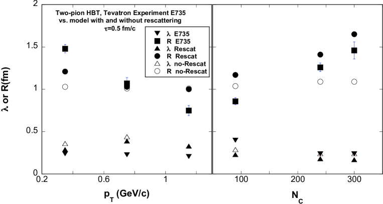
Figure 5: Comparisons of Gaussian fit parameters for pions between Tevatron data (Experiment E735) and model predictions with and without rescattering at $\tau=0.5$ fm/c versus $p_{T}$ and $N_{C}$.

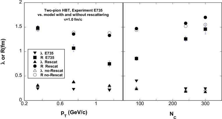
Figure 6: Comparisons of Gaussian fit parameters for pions between Tevatron data (Experiment E735) and model predictions with and without rescattering at $\tau=1.0$ fm/c versus $p_{T}$ and $N_{C}$.

Figures 1 - 8 present results of the model for $\sqrt{s}=1.8$ TeV $p-\bar{p}$ collisions. Comparisons with E735 Gaussian fit parameters are shown in Figures 4 - 8.

Figure 1 shows model rapidity and $p_{T}$ distribution plots for all final-state particles (i.e. pions, kaons, and nucleons) for three cases: 1) directly from PYTHIA, 2) PYTHIA with a $\eta-p_{T}$ “hole”, and 3) same as 2) but with rescattering turned on and $\tau=0.1$ fm/c. For case 1), PYTHIA events are directly run through the model code without any other process applied to them except to decay $\Lambda$s, and the $\rho$, $\omega$, $\eta$, ${\eta}^{\prime}$, $\phi$, $\Delta$, and $K^{*}$ resonances, i.e. “pure PYTHIA”. Since PYTHIA has been tuned to agree reasonably well with existing experimental data, including Tevatron data, these distributions should remain at least approximately the same after rescattering has been turned on. This turns out not to be the case for $\tau=0.1$ fm/c, since It is found that if “pure” PYTHIA events are input into the calculation with rescattering turned on, a small peak results in the $\eta$ distribution near midrapidity and the $p_{T}$ distribution is overly enhanced compared with “pure” PYTHIA. This gives the first suggestion that final-state hadronic rescattering can play a noticeable role in these collisions. In an effort to compensate for the rescattering effects so as to give approximate agreement with the “pure” PYTHIA distributions, a $\eta-p_{T}$ “hole” is inserted in the input PYTHIA events before rescattering, as shown, and the rescattering then fills the “hole” to approximately agree with the “pure” PYTHIA distributions, also shown in Figure 1. For this case, the “hole” is defined by randomly throwing away 5% of the particles in the input PYTHIA events in the $y-p_{T}$ region $-1<y<1$ and $p_{T}>0.5$ GeV/c. For the larger values of $\tau$ studied, i.e. $\tau=0.5$ and $1.0$ fm/c, less rescattering takes place due to the larger initial hadronization volume and thus lower initial particle density and the “hole” depth is reduced, using the prescription $5\%(0.1/\tau)$ to define it. The justification for using this “hole” method is that reasonable agreement with the “pure” PYTHIA distributions is obtained with recattering turned on. Note that including or not including the “hole” has only a small effect on the HBT results presented later.

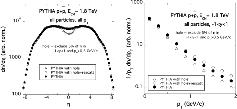
Figure 1: Pseudorapidity and $p_{T}$ distributions from PYTHIA for $p-\bar{p}$ collisions at $\sqrt{s}=1.8$ TeV for three cases: 1) directly from PYTHIA, 2) PYTHIA with $\eta-p_{T}$ “hole”, and 3) same as 2) but with rescattering turned on and $\tau=0.1$ fm/c.

Figure 2 shows sample two-pion correlation functions from the rescattering model for $\tau=$ 0.1, 0.5, and 1.0 fm/c with fits to the Gaussian function, Eq. (5), for $\sqrt{s}=1.8$ TeV $p-\bar{p}$ collisions. A comparison is also made for the $\tau=0.1$ fm/c case between two $p_{T}$ cuts on the pions, i.e. $0.2<p_{T}<0.5$ GeV/c and $p_{T}>1$ GeV/c. As seen, the Gaussian fits qualitatively reproduce the trends of the model correlation functions, but do not well represent all of the details of the shapes, which include an exponential-like shape for $\tau=0.1$ fm/c and some oscillatory behavior for $\tau=0.5$ and $1.0$ fm/c. The oscillatory behavior is a feature of the delta-function assumption of $\tau$, which becomes more prominent for larger values of $\tau$ csorgo .

Figure 3 shows sample correlation functions where the model is run with a uniform distribution of $\tau$ as a test, for the two cases $\tau<0.2$ fm/c and $\tau<1.0$ fm/c. As seen by comparing Figures 2 and 3, these cases closely resemble the correlation functions for $\tau=0.1$ and $\tau=0.5$ fm/c, respectively. A more complete comparison is shown later.

Figure 2: Sample two-pion correlation functions from the rescattering model for $\tau=$ 0.1, 0.5, and 1.0 fm/c with fits to the Gaussian function for $\sqrt{s}=1.8$ TeV $p-\bar{p}$ collisions.

Figure 3: Sample two-pion correlation functions from the rescattering model for $\tau<0.2$ and $\tau<1.0$ fm/c with fits to the Gaussian function for $\sqrt{s}=1.8$ TeV $p-\bar{p}$ collisions.

Figure 4-6 show comparisons of Gaussian fit parameters for pions between Tevatron data (Experiment E735) and model predictions with and without rescattering at $\tau=0.1,0.5$ and $1.0$ fm/c, respectively, versus $p_{T}$ and $N_{C}$. As anticipated earlier, rescattering is seen to have the greatest effect on the fit parameters for the smallest value of $\tau$, $\tau=0.1$ fm/c, becoming less important as $\tau$ increases until it is seen to have an almost negligible effect at $\tau=1.0$ fm/c. All three $\tau$ cases (with rescattering) do an adequate job of describing the flat dependence of $\lambda$ on $p_{T}$ and $N_{C}$ seen in E735. It is also seen that the overall trends of the E735 $R$ dependencies, i.e. decreasing with increasing $p_{T}$ and increasing with increasing $N_{C}$, are best reproduced by the $\tau=0.1$ fm/c case with rescattering turned on, the larger $\tau$ model predictions becoming progressively flatter with increasing $\tau$. Another feature found in the correlation functions of the higher $\tau$ values not found in the E735 correlation functions is the oscillation in the baseline seen in Figure 2. No such oscillation appears for the $\tau=0.1$ fm/c case, in agreement with E735.

Figures 7 and 8 show results for running the model with flat distributions of $\tau$, i.e. $\tau<0.2$ fm/c and $\tau<1.0$ fm/c, and comparing with the delta-function cases $\tau=0.1$ and $0.5$ fm/c, which are the average values of the two flat ranges, respectively, with rescattering turned on, and compared with E735. As seen, the fit parameters for the flat $\tau$ distributions give virtually the same results as the delta-function $\tau$ distributions, demonstrating that either method of running the model gives almost identical results.

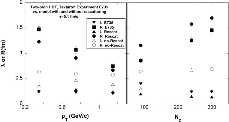
Figure 4: Comparisons of Gaussian fit parameters for pions between Tevatron data (Experiment E735) and model predictions with and without rescattering at $\tau=0.1$ fm/c versus $p_{T}$ and $N_{C}$.

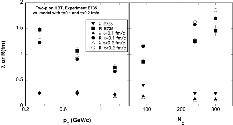
Figure 7: Comparisons of Gaussian fit parameters for pions between Tevatron data (Experiment E735) and model predictions with rescattering for $\tau=0.1$ fm/c and $\tau<0.2$ fm/c versus $p_{T}$ and $N_{C}$.

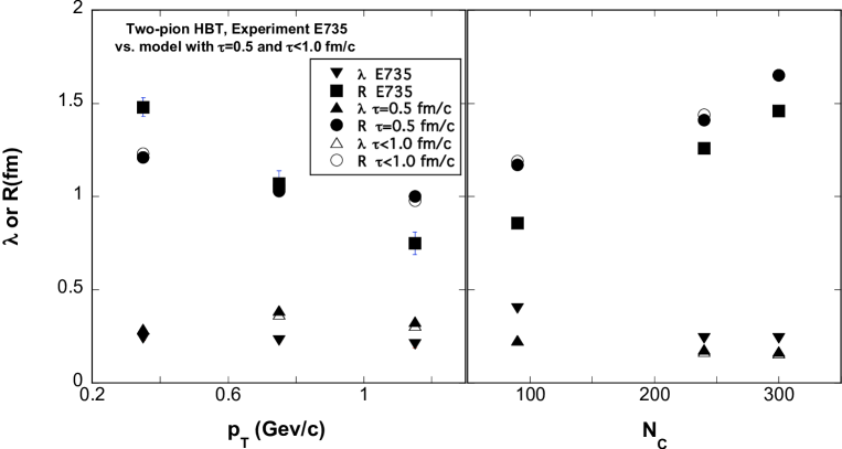
Figure 8: Comparisons of Gaussian fit parameters for pions between Tevatron data (Experiment E735) and model predictions with rescattering for $\tau=0.5$ fm/c and $\tau<1.0$ fm/c versus $p_{T}$ and $N_{C}$.

Summarizing this section, the main result of the comparison of the HBT fit parameters from the present model with those from Tevatron experiment E735 shown above is that the $\tau=0.1$ fm/c case best describes the trends of the fit parameters on $p_{T}$ and $N_{C}$. This would seem to imply that the hadronization time in these collisions is short, i.e. $\tau<<1$ fm/c, and, as a consequence of this, large hadron densities exist at the early stage of the collision resulting in significatnt hadronic rescattering effects.

III.2 Predictions for p-p collisions at $\sqrt{s}=14$ TeV

Figures 9 - 13 present results from the present model calculations for $p-p$ collisions at $\sqrt{s}=14$ TeV to simulate full-energy LHC collisions. All calculations shown are for pions at mid-rapidity, i.e. $-1<y<1$. Several values of $\tau$ and cuts on particle multiplicity and pion $p_{T}$ are studied. In the results shown below, multiplicity is defined as the total multiplicity of pions, kaons, and nucleons of all charge states for all rapidity and $p_{T}$ in a collision. In order to compare with future experiments, the approximate correspondence between the total multiplicity bins used and the more experiment-friendly average detectable ($p_{T}>100$ MeV/c) mid-rapidity ($-1<y<1$) charged particle multiplicity is shown in Table I. Also shown in Table I is the fraction of minimum bias events corresponding to each multiplicity bin. From this it is seen that all multiplicities used are predicted to be easily experimentally accessible.

Table 1: Approximate correspondence between the total multiplicity bins used in the present calculations and the average detectable mid-rapidity charged multiplicity. The fraction of minimum bias events is also shown.

Total mult.bin	Ave.detectable charged	fraction of
m	particle mult.at mid-y	MB events
0-100	5	0.42
100-200	14	0.34
200-300	26	0.14
300-400	41	0.069
400-500	58	0.026
500-600	79	0.0042
$>$ 300	47	0.093

The following choices were made for the conditions used in the model calculations in generating the LHC predictions:

• Based on the comparisons presented above between the model and E735 results, predictions using the “delta-function” model for $\tau$ for the cases $\tau=0.1$ and $0.5$ fm/c were made. As shown above for the Tevatron calculations, these cases give almost identical results as for the “flat-distribution” model for $\tau<0.2$ and $1.0$ fm/c. Although the closest agreement between the present rescattering calculations and E735 results was obtained for the $\tau=0.1$ fm/c case, predictions are also included for $\tau=0.5$ fm/c since the hadronization time for $\sqrt{s}=14$ TeV collisions may be larger than that for $\sqrt{s}=1.8$ TeV.

• Employ the same “$\eta-p_{T}$ hole” method as for the Tevatron calculations, i.e. the “hole” is defined by randomly throwing away 5% of the particles in the input PYTHIA events in the $y-p_{T}$ region $-1<y<1$ and $p_{T}>0.5$ GeV/c for the $\tau=0.1$ fm/c case, and scaled down accordingly for the $\tau=0.5$ fm/c case. Comparisons of pseudorapidity and $p_{T}$ distributions between PYTHIA run for the maximum LHC energy and PYTHIA with the “hole” and rescattering turned on for $\tau=0.1$ are shown in Figure 9.

• To extract the pion HBT fit parameters from the invariant correlation functions generated by the model, use Eq.(6). As described above, this is to better characterize the finer features of the correlation functions and thus get better fits to the calculations. Figures 10 and 11 show fits to sample model-generated correlation functions for the cases $\tau=0.1$ and $0.5$ fm/c, respectively. As seen, the fits are in general quite good.

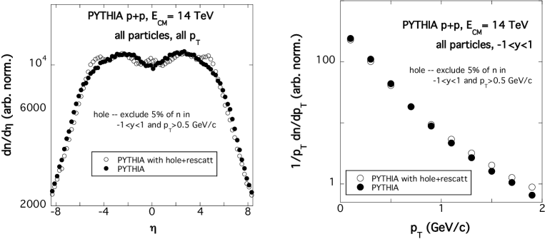
Figure 9: Pseudorapidity and $p_{T}$ distributions from PYTHIA for $p-p$ collisions at $\sqrt{s}=14$ TeV for two cases: 1) directly from PYTHIA, and 2) PYTHIA with $\eta-p_{T}$ “hole” and with rescattering turned on for the case $\tau=0.1$ fm/c.

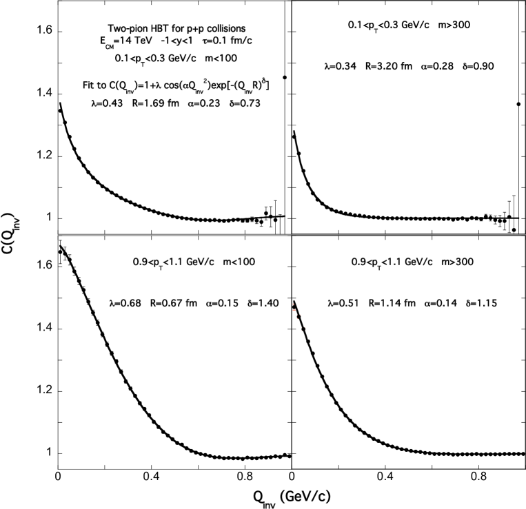
Figure 10: Sample two-pion correlation functions from the rescattering model for $\tau=$ 0.1 fm/c with fits to the general function (i.e. Eq.(6)) for $\sqrt{s}=14$ TeV $p-p$ collisions.

Figure 11: Sample two-pion correlation functions from the rescattering model for $\tau=$ 0.5 fm/c with fits to the general function (i.e. Eq. (6)) for $\sqrt{s}=14$ TeV $p-p$ collisions.

Figures 12 and 13 show the predicted dependences of the fit parameters on $p_{T}$ and total multiplicity, $m$, for the cases $\tau=0.1$ and $0.5$ fm/c, respectively for $\sqrt{s}=14$ TeV $p-p$ collisions. Plots are made with low and high multiplicity cuts, i.e. $m<100$ and $m>300$, and low and high $p_{T}$ cuts, i.e. $0.1<p_{T}<0.3$ GeV/c and $0.9<p_{T}<1.1$ GeV/c. The behaviors of the fit parameters seen in Figures 12 and 13 are discussed separately below.

III.2.1 $R$-parameter

The $R$-parameter, which is related to the “size” of the pion-emitting source (see Eq.(7)), is seen to have the largest variation for different kinematical cuts, i.e. the strongest dependencies on $p_{T}$ and $m$. These are greatest for $\tau=0.1$ fm/c since they are almost completely due to rescattering effects. In Figure 12 it is seen that for the proper kinematical cuts $R$ can be made to increase by a factor of three for increasing $m$ or decrease by a factor of three for increasing $p_{T}$. Experimental observation of such strong variations in $R$ would be a convincing signature for the presence of significant rescattering effects and therefore a short hadronization time.

III.2.2 $\lambda$-parameter

The $\lambda$-parameter, which is related to the “strength” of the HBT effect, is seen to have weak dependences on the kinematical cuts and to have a similar magnitude for both the $\tau=0.1$ and $0.5$ fm/c cases. It tends to have a magnitude such that $\lambda<0.5$, which is mostly due to the presence of long-lived resonances in the model calculations which tend to suppress it. Though weak, it has a slightly increasing tendency for increasing $p_{T}$ and decreasing tendency for increasing $m$, which is opposite the directions of the dependencies for $R$.

III.2.3 $\alpha$-parameter

The $\alpha$-parameter, which is seen in Eq.(6) to be related to oscillatory behavior of the correlation function, is seen to mostly depend on the value of $\tau$. As also seen in Figures 10 and 11, it is small, i.e. $\alpha<0.2$, for $\tau=0.1$ fm/c and large, i.e. $\alpha\sim 0.5-0.6$, for $\tau=0.5$ fm/c. The connection between $\alpha$ and $\tau$ for the simple case of a delta-function hadronization time can indeed be shown to be $\tau\sim\alpha$ csorgo . Experimental observation of oscillations in the correlation function, i.e. large $\alpha$ values, would be evidence for a larger value of the hadronization time, i.e. $\tau>0.5$ fm/c.

III.2.4 $\delta$-parameter

As seen in Eq.(6), the $\delta$-parameter is related to how “exponential-like” ($\delta\sim 1$) or “Gaussian-like” ($\delta\sim 2$) the correlation function appears. As with $\lambda$, it is seen to have weak dependences on the kinematical cuts, to have a similar magnitude for both the $\tau=0.1$ and $0.5$ fm/c cases, and to have dependencies which are opposite to the directions of the dependencies for $R$. It tends to have values in the range $0.7<\delta<1.5$.

Figure 12: General function fit parameters versus $p_{T}$ and particle multiplicity from the rescattering model with $\tau=0.1$ fm/c for several multiplicity and $p_{T}$ cuts for $p-p$ collisions at $\sqrt{s}=14$ TeV. The dashed lines are drawn to guide the eye.

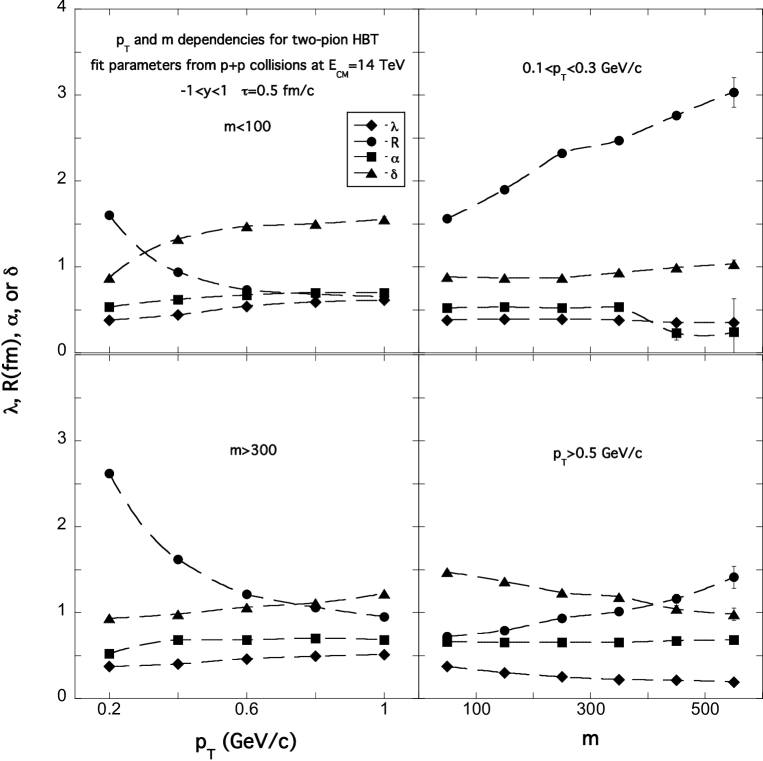
Figure 13: General function fit parameters versus $p_{T}$ and particle multiplicity from the rescattering model with $\tau=0.5$ fm/c for several multiplicity and $p_{T}$ cuts for $p-p$ collisions at $\sqrt{s}=14$ TeV. The dashed lines are drawn to guide the eye.

IV Conclusions

A simple model assuming a uniform hadronization proper time and including final-state hadronic rescattering has been used to predict two-pion HBT fit parameters for $p-\bar{p}$ collisions at $\sqrt{s}=1.8$ TeV and $p-p$ collisions at 14 TeV. For small values of $\tau$, i.e. $\tau<0.5$ fm/c, it is found that rescattering has a significant influence on the fit parameters. Comparing the model predictions with $p-\bar{p}$ experimental results at $\sqrt{s}=1.8$ TeV, the closest agreement is found for small $\tau$, i.e. $\tau\sim 0.1$ fm/c. This suggests that 1) final-state hadronic rescattering is already important at $\sqrt{s}=1.8$ TeV and 2) hadronization times are short.

As is seen in the above figures, there are significant differences in the magnitudes and dependences on kinematical variables for the general fit parameters evaluated at different $\tau$-values in the model calculations carried out for $\sqrt{s}=14$ TeV $p-p$ collisions. Comparisons of these results with actual future data from the LHC will be able to establish a) if this simple model describes the data in even a qualitative way and b) if so, the scale of the hadronization time in these collisions.

- (1) R. Hanbury Brown and R. Q. Twiss, Nature 177, 27 (1956).
- (2) G. Goldhaber, S. Goldhaber, W. Lee, and A. Pais, Phys. Rev.120, 300 (1960).
- (3) M. A. Lisa, S. Pratt, R. Soltz and U. Wiedemann, Ann. Rev. Nucl. Part. Sci. 55, 357 (2005).
- (4) T. J. Humanic, Int. J. Mod. Phys. E 15, 197 (2006).
- (5) T. Alexopoulos et al., Phys. Rev. D 48, 1931 (1993).
- (6) G. Paic and P. K. Skowronski, J. Phys. G 31, 1045 (2005).
- (7) T. Sjostrand, L. Lonnblad, S. Mrenna and P. Skands, arXiv:hep-ph/0308153.
- (8) S. Dimopoulos and G. Landsberg, Phys. Rev. Lett. 87, 161602 (2001).
- (9) T. Csorgo and J. Zimanyi, Nucl. Phys. A 512, 588 (1990).
- (10) T. Novak [L3 Collaboration], AIP Conf. Proc. 828, 539 (2006).
- (11) T. J. Humanic, Phys. Rev. C 57, 866 (1998).
- (12) M. Prakash, M. Prakash, R. Venugopalan and G. Welke, Phys. Rept. 227, 321 (1993).
- (13) W. M. Yao et al. [Particle Data Group], J. Phys. G 33, 1 (2006).
- (14) T. J. Humanic, Phys. Rev. C 73, 054902 (2006).
- (15) T. J. Humanic, Phys. Rev. C 34, 191 (1986).