The Phase Diagram of Neutral Quark Matter
Dissertation
zur Erlangung des Doktorgrades
der Naturwissenschaften
vorgelegt beim Fachbereich Physik
der Johann Wolfgang Goethe - Universität
in Frankfurt am Main
von
Stefan Bernhard Rüster
aus Alzenau in Ufr.
Frankfurt 2006
(D 30)

vom Fachbereich Physik der
Johann Wolfgang Goethe - Universität als Dissertation angenommen.
Dekan: Prof. Dr. Aßmus
Gutachter: Prof. Dr. Rischke und HD PD Dr. Schaffner-Bielich
Datum der Disputation: 14. Dezember 2006

Abstract

In this thesis, I study the phase diagram of dense, locally neutral three-flavor quark matter as a function of the strange quark mass, the quark chemical potential, and the temperature, employing a general nine-parameter ansatz for the gap matrix. At zero temperature and small values of the strange quark mass, the ground state of quark matter corresponds to the color–flavor-locked (CFL) phase. At some critical value of the strange quark mass, this is replaced by the recently proposed gapless CFL (gCFL) phase. I also find several other phases, for instance, a metallic CFL (mCFL) phase, a so-called uSC phase where all colors of up quarks are paired, as well as the standard two-flavor color-superconducting (2SC) phase and the gapless 2SC (g2SC) phase.

I also study the phase diagram of dense, locally neutral three-flavor quark matter within the framework of a Nambu–Jona-Lasinio (NJL) model. In the analysis, dynamically generated quark masses are taken into account self-consistently. The phase diagram in the plane of temperature and quark chemical potential is presented. The results for two qualitatively different regimes, intermediate and strong diquark coupling strength, are presented. It is shown that the role of gapless phases diminishes with increasing diquark coupling strength.

In addition, I study the effect of neutrino trapping on the phase diagram of dense, locally neutral three-flavor quark matter within the same NJL model. The phase diagrams in the plane of temperature and quark chemical potential, as well as in the plane of temperature and lepton-number chemical potential are presented. I show that neutrino trapping favors two-flavor color superconductivity and disfavors the color–flavor-locked phase at intermediate densities of matter. At the same time, the location of the critical line separating the two-flavor color-superconducting phase and the normal phase of quark matter is little affected by the presence of neutrinos. The implications of these results for the evolution of protoneutron stars are briefly discussed.

Chapter 1 Introduction

The phase diagram of neutral quark matter was poorly understood as I began with the research on this topic in 2003. The task of my thesis was therefore to illuminate the phase structure of neutral quark matter. A phase diagram is a two-dimensional diagram with axes representing the temperature and the chemical potential, the density, or other similar quantities. Therefore, phase diagrams tell us in which state is a system for a given temperature and a given chemical potential. Besides, they contain the information at which temperatures and which chemical potentials transitions to other phases occur. Such phase transitions can be of first or second order, or simply crossovers. This depends on the order parameter of the system. If it changes discontinuously, then a first, otherwise a second-order phase transition or a crossover appears.

In Sec. 1.1, I show the status of knowledge of the phase diagram of strongly interacting matter before I began with my research for this thesis in 2003. As one can see, the phase diagram of neutral quark matter was indeed poorly understood at that time. In Sec. 1.2, I discuss the behavior of sufficiently cold and dense quark matter, namely that quark matter is color-superconducting and that color-superconducting quark matter appears in several phases. The most important color-superconducting phases are presented in Sec. 1.2. In Sec. 1.3, I give a short but comprehensive introduction into stellar evolution because the cores of neutron stars are the only places in nature where one expects neutral color-superconducting quark matter. Thereby, it will become clear what a star is, how it is formed, which processes happen in a star, and what are the final stages of stellar evolution. In Sec. 1.4, I focus on neutron stars. It is explained how neutron stars are formed, of which matter they consist, and I present the structure of neutron stars. In Sec. 1.5, it is argued why neutral color-superconducting quark matter is expected to occur in neutron star cores.

In Chapter 2, I present the calculations to obtain the pressure for neutral color-superconducting quark matter, and I show the phase diagram of neutral quark matter. With this one can predict in which state neutral quark matter is in the cores of neutron stars.

In Chapter 3, I summarize the results and conclude my thesis.

Important definitions and useful formulae can be found in the Appendix.

1.1 The phase diagram of strongly interacting matter

The fundamental theory of the strong interaction is called quantum chromodynamics (QCD). The participants of the strong interaction are the elements of hadronic matter, the quarks and gluons. Quarks interact via gluons because both particle species carry so-called color charges (red, green, and blue) which are responsible for the interaction. In our everyday life, we do not see quarks or gluons because they are confined into hadrons. This is because the quark interaction caused by gluons is so strong that they cannot exist as free particles. QCD is an asymptotically free theory [1]. At high temperatures or densities, the quarks are deconfined because their mutual distances decrease and the exchanged momenta increase so that the interaction becomes sufficiently weak [2]. The state of deconfined quarks is called the quark-gluon plasma (QGP). Such a phase certainly existed in the early universe which was very hot, but close to net-baryon free. Nowadays, the only place in nature where a QGP may exist is in the interior of neutron stars. Here, the density is extremely high and the temperature low. The third place where an artificially created QGP could appear is in heavy-ion collisions. The temperatures and densities which are reached by the collisions depend on the bombarding energies.

Figure 1.1: The status of knowledge of the phase diagram of strongly interacting matter as I began with the research on this topic for my thesis in 2003 [3]. Note that this phase diagram is drawn schematically.

In Fig. 1.1, I show the status of knowledge of the phase diagram of strongly interacting matter in the plane of temperature $T$ and quark chemical potential $\mu$ before I began with the research for my thesis in 2003 [3]. There is a phase transition at the point $(T,\mu)\simeq(0,308)$ MeV which separates the gaseous nuclear phase at lower $\mu$ from the liquid nuclear phase at higher $\mu$. The nuclear liquid-gas transition [4] which is a first-order phase transition starts from this point and disappears in a critical endpoint at $T\sim 10$ MeV and slightly lower quark chemical potential. In this endpoint, the transition is of second order. Above the endpoint, there is no distinction between these two phases. The transition point at zero temperature is easily found because nucleons of infinite and isospin-symmetric nuclear matter in the ground state at normal nuclear density $n_{0}\simeq 0.15$ fm^-3 are bound by 16 MeV (if one neglects the repulsive Coulomb forces). The energy per baryon or the energy density per baryon density respectively is given by $E/N_{B}=\epsilon/n_{B}=m_{n}-16$ MeV where $m_{n}\simeq 940$ MeV is the rest mass of the baryon. By using the thermodynamic relation $\epsilon=Ts-p+\mu n$, one obtains for the ground state of nuclear matter where the pressure $p=0$ that the baryon chemical potential is identical to the energy per baryon $\mu_{B}\equiv\epsilon/n_{B}\simeq 924$ MeV. Since a baryon contains three quarks, the quark chemical potential is one third of the baryon chemical potential, $\mu=\mu_{B}/3$. This leads to the result $\mu\simeq 308$ MeV for the transition point at zero temperature.

Nuclear matter consists of droplets which is the most energetically preferred form for nuclear matter in the low-density and low-temperature regime of the phase diagram. In the gaseous phase at low density and nonzero temperature, nucleons will be evaporated from the surface of the droplets so that there is a mixture of droplets and nucleons. As soon as the chemical potential exceeds the one corresponding to the nuclear liquid-gas phase transition, only droplets of nuclear matter but no evaporated nucleons will appear.

At low quark chemical potentials, strongly interacting matter is in the hadronic phase. At nonzero temperature, nuclear matter not only consists of nucleons but also of thermally excited hadrons. Therefore, at low quark chemical potentials, a large amount of pions can be found. By increasing the temperature, the system passes the quark-hadron transition line and enters the regime of the QGP. The critical endpoint of the transition line at $(T,\mu)=(162\pm 2,120\pm 14)$ MeV obtained by lattice QCD calculations [5] depends on the value of the quark masses and is of second order. For smaller quark chemical potentials, the transition becomes a crossover, and there is no real distinction between hadronic matter and the QGP. For larger quark chemical potentials, the transition is a line of first-order phase transitions that separates the hadronic phase from the QGP. But it is not known whether the line of first-order phase transitions goes all the way down to zero temperature. If so, also the precise value of the quark chemical potential for the phase transition at zero temperature is unknown. One should mention that these lattice QCD calculations are not very reliable at nonzero quark chemical potential. In addition, these calculations are done with probably unrealistic large quark masses and on fairly small lattice sizes. For smaller quark masses, the endpoint should move towards the temperature axis. By increasing the quark chemical potential, the nucleons will be packed denser and denser until the quark-hadron phase transition is reached. As soon as the quark chemical potential exceeds this transition line, the system becomes a color superconductor at low temperatures or a QGP which is in the normal conducting phase (NQ) at high temperatures.

At large quark chemical potentials and low temperatures, quark matter becomes a color superconductor. In this thesis, I shall focus on this part of the phase diagram and its transitions to the hadronic phase and to normal quark matter. The reader will see that there exist various color-superconducting phases and that this thesis will update the phase diagram of strongly interacting matter in the quark regime.

1.2 Color superconductivity

Quarks are spin-$\frac{1}{2}$ fermions and therefore obey the Pauli principle which requires that one quantum state is occupied by only one fermion. At zero temperature, non-interacting quarks occupy all available quantum states with lowest possible energies. This behavior is expressed with the Fermi-Dirac distribution function for zero temperature,

$$f_{F}\left(\mathbf{k}\right)=\theta\left(\mu-E_{\mathbf{k}}\right)\;,$$ (1.1)

where $E_{\mathbf{k}}=\sqrt{k^{2}+m^{2}}$ is the energy of a free massive quark. All states with momenta $k\equiv|\mathbf{k}|$ which are less than the Fermi momentum $k_{F}=\sqrt{\mu^{2}-m^{2}}$ are occupied. The states with momenta larger than the Fermi momentum are empty. The pressure for massive non-interacting quarks at zero temperature is given by

$$p=\frac{g}{6\pi^{2}}\int_{0}^{\infty}\mathrm{d}k\,\frac{k^{4}}{E_{\mathbf{k}}}f_{F}\left(\mathbf{k}\right)-B=\frac{g}{6\pi^{2}}\int_{0}^{k_{F}}\mathrm{d}k\,\frac{k^{4}}{E_{\mathbf{k}}}-B\;,$$ (1.2)

where $g=2N_{c}N_{f}$ is the degeneracy factor in which $N_{c}$ is the number of colors, and $N_{f}$ the number of flavors. The factor two comes because of spin degeneracy. The bag constant $B$ assigns a nonzero contribution to the vacuum pressure and, in this way, provides the simplest modelling of quark confinement in QCD [6]. A typical value for the bag pressure is $B^{1/4}=0.17$ GeV which is used in Refs. [7, 8]. In the limit of zero mass and zero temperature, the pressure of non-interacting quarks reads

$$p=\frac{g}{24\pi^{2}}\mu^{4}-B\;.$$ (1.3)

This is the case of non-interacting quarks. What happens when the quark interaction is switched on?

At asymptotically large quark chemical potentials, the strong coupling constant becomes small so that the dominant interaction between quarks is given by single-gluon exchange. The quark-quark scattering amplitude in the one-gluon exchange approximation is proportional to

$$\sum_{A=1}^{N_{c}^{2}-1}T_{ki}^{A}T_{lj}^{A}=-\frac{N_{c}+1}{4N_{c}}\left(\delta_{jk}\delta_{il}-\delta_{ik}\delta_{jl}\right)+\frac{N_{c}-1}{4N_{c}}\left(\delta_{jk}\delta_{il}-\delta_{ik}\delta_{jl}\right)\;,$$ (1.4)

where $i$, $j$ are the colors of the incoming, and $k$, $l$ those of the outgoing channel. The first term in this equation is antisymmetric and corresponds to the antitriplet channel which is responsible for the dominant attractive interaction while the second term is symmetric and corresponds to the sextet channel which is responsible for the repulsive interaction, see Fig. 1.2.

Figure 1.2: The diagrammatic representation of the one-gluon exchange interaction between two quarks in QCD [9].

Therefore, the antitriplet channel with its dominant attractive interaction ensures that quarks with large momenta (quarks near the Fermi surface) form bosonic quark Cooper pairs [10, 11, 12]. This state is called a color superconductor in analogy to superconductivity of electrons [13]. The arguments how color superconductivity is created hold rigorously at asymptotically large densities. The highest densities of nuclear matter that can be achieved in colliders or that occur in nature in the cores of neutron stars are of the order of ten times the nuclear matter ground state density at which the quark chemical potential approximately amounts to $\mu\simeq 500$ MeV. Nevertheless, calculations in the framework of an NJL model [14] show that color superconductivity also occurs at moderate densities and is not limited to asymptotically large densities [15].

As a consequence of (color) superconductivity, there exists at least one gap in the quasiparticle spectra. Such a color-superconducting gap (parameter) $\Delta$ is a diquark condensate which is defined as an expectation value,

$$\Delta\propto\langle\psi^{T}\mathcal{O}\psi\rangle\;,$$ (1.5)

where the operator,

$$\mathcal{O}=\mathcal{O}_{\mathrm{color}}\otimes\mathcal{O}_{\mathrm{flavor}}\otimes\mathcal{O}_{\mathrm{Dirac}}\;,$$ (1.6)

acts on the quark spinor field $\psi$ in color, flavor, and Dirac space. The color-superconducting gap parameters $\Delta_{i}$ are zero in normal quark matter and nonzero ($\Delta_{i}\sim 100$ MeV) in color-superconducting quark matter, and they are equal to one half of the binding energy of a quark Cooper pair. The values of the gap parameters can be obtained by solving the gap equations

$$\frac{\partial p_{\mathrm{CSC}}}{\partial\Delta_{i}}=0\;,$$ (1.7)

where $p_{\mathrm{CSC}}$ is the pressure of color-superconducting quark matter.

In ordinary superconductors, the $[U(1)_{\mathrm{em}}]$ gauge symmetry is broken so that the photons become massive. (Throughout this thesis, I indicate local, i.e., gauged, symmetries by square brackets.) This leads to the so-called Meissner effect, the expulsion of magnetic fields from the superconducting region. In a color superconductor, the $[SU(3)_{c}]$ color gauge symmetry is broken so that some of the eight types of gluons become massive. In an ordinary superconductor as well as in a color superconductor, thermal motion will break up Cooper pairs and therefore destroy the (color-)superconducting state. In a color superconductor, this transition is of second order and happens at the critical temperature

$$T_{c}^{\mathrm{BCS}}=\frac{\mathrm{e}^{\gamma}}{\pi}\Delta_{0}\simeq 0.567\Delta_{0}$$ (1.8)

where $\Delta_{0}$ is the color-superconducting gap at zero temperature, and $\gamma\simeq 0.577$ the Euler-Mascheroni constant.

But there are also differences when one compares superconductivity with color superconductivity: the electrons in superconductors first have to overcome their repulsive Coulomb forces in order to form Cooper pairs while in color superconductors, the formation of quark Cooper pairs is much simpler because there already exists the attractive interaction in the antitriplet channel. Quarks, unlike electrons, come in various flavors, see Table 1.1, and carry color charges. Because of this latter quark property, superconductivity of quarks is called color superconductivity.

Flavor	Mass [MeV]	$Q$ [e]
up	$2\ldots 8$	$2/3$
down	$5\ldots 15$	$-1/3$
strange	$100\ldots 300$	$-1/3$
charm	$1300\ldots 1700$	$2/3$
bottom	$4700\ldots 5300$	$-1/3$
top	$174000\pm 17000$	$2/3$

Table 1.1: The masses and electric charges of the quark flavors [16]. The abbreviation for the respective quark is written in the bold Roman font. There also exists the corresponding antiquark for each flavor with charge $-Q$. They are not shown here.

The quarks in color-superconducting quark matter are called quasiparticles or quasiquarks, respectively. One only needs to consider the lightest quarks (up, down, and strange) for color-superconducting quark matter, because the heavy quarks (charm, bottom, and top) are so massive that their occurrence in quark matter is extremely unlikely for the densities and temperatures under consideration.

The color and flavor structure of the condensate of quark Cooper pairs which is also called the color-flavor gap matrix depends on which quark flavors participate in pairing and which total spin $J$ the Cooper pairs have. For $J=0$, the spin part of the quark Cooper pair wavefunction is antisymmetric, and therefore the color-flavor part has to be symmetric in order to fulfill the requirement of overall antisymmetry. Since quarks pair in the antisymmetric color-antitriplet channel, the flavor part of the wavefunction also has to be antisymmetric.

1.2.1 The 2SC phase

In order to fulfill the symmetry requirements, at least two quarks of different flavor are needed for the $J=0$ case. Therefore, the simplest ansatz for the color-flavor gap matrix has the form:

$$\Delta_{ij}^{fg}=\epsilon_{ijk}\epsilon^{fg}\Delta_{k}\;,$$ (1.9)

where the order parameter

$$\Delta_{k}=\delta_{k3}\Delta$$ (1.10)

conventionally points in anti-blue color direction. Together with the Dirac part, the gap matrix reads

$$\Phi_{ij}^{fg}=\gamma_{5}\Delta_{ij}^{fg}\;.$$ (1.11)

This is the so-called 2SC phase which is an abbreviation for 2-flavor color superconductor. The color indices $i$ and $j$ run from one to the number of colors $N_{c}$ which is equal to three. The flavor indices $f$ and $g$ run from one to the number of flavors $N_{f}$ participating in pairing which is equal to two in the 2SC phase. In this phase, red up quarks pair with green down quarks, and red down quarks pair with green up quarks, and form anti-blue quark Cooper pairs.

The blue quarks remain unpaired and therefore cause gapless quasiparticles. These quasiparticles give dominant contributions to the specific heat and to the electrical and heat conductivities. They are also responsible for a large neutrino emissivity produced by the $\beta$ processes $\mathrm{d_{b}\rightarrow u_{b}+e^{-}+\bar{\nu}_{e}}$ and $\mathrm{u_{b}+e^{-}\rightarrow d_{b}+\nu_{\mathrm{e}}}$. The other four quasiparticles and quasiantiparticles fulfill the dispersion relation

$$\epsilon_{\mathbf{k}}^{e}=\sqrt{\left(E_{\mathbf{k}}-e\mu\right)^{2}+\left|\Delta\right|^{2}}\;,$$ (1.12)

where $\Delta$ is the gap, and $e=\pm$ stands for quasiparticles and quasiantiparticles, respectively. At small temperatures ($T\ll\Delta$) , the contributions of these quasiparticles to all transport and many thermodynamic quantities are suppressed by the exponentially small factor $\exp\left(-\Delta/T\right)$ [9]. The gluons are bosons and therefore, their number density is small at low temperature. In the 2SC phase, the $[SU(3)_{c}]$ gauge symmetry is broken to $[SU(2)_{c}]$. Consequently, there are $8-3=5$ broken generators. They represent five gluons which are gapped because of the color Meissner mass. Therefore, gluons have only tiny influence on the properties of quark matter in the 2SC phase. The unpaired blue quarks are responsible for the absence of baryon superfluidity. Only the anti-blue quasiparticles carry a nonzero baryon number. This can be seen by the generator of baryon number conservation,

$$\tilde{B}=B-\frac{2}{\sqrt{3}}T_{8}=\mathrm{diag}_{c}\left(0,0,1\right)\;,$$ (1.13)

where $T_{8}$ is the eighth generator of the $[SU(3)_{c}]$ group. The electromagnetic generator of the unbroken $[\tilde{U}(1)_{\mathrm{em}}]$ gauge symmetry in the 2SC phase is

$$\tilde{Q}=Q-\frac{1}{\sqrt{3}}T_{8}\;,\quad\tilde{Q}^{r}_{u}=\tilde{Q}^{g}_{u}=\frac{1}{2}\;,\quad\tilde{Q}^{b}_{u}=1\;,\quad\tilde{Q}^{r}_{d}=\tilde{Q}^{g}_{d}=-\frac{1}{2}\;,\quad\tilde{Q}^{b}_{d}=0\;.$$ (1.14)

where $Q=\mathrm{diag}_{f}\left(\frac{2}{3},-\frac{1}{3}\right)$ is the electromagnetic generator of the $[U(1)_{\mathrm{em}}]$ gauge symmetry in vacuum. The gauge boson of $[\tilde{U}(1)_{\mathrm{em}}]$ is the medium photon. Therefore, there exists no electromagnetic Meissner effect in the 2SC phase and that is the reason why a magnetic field would not be expelled from the color-superconducting region. The 2SC phase is a so-called $\tilde{Q}$-conductor because its electrical conductivity is large. The $\tilde{Q}$ charge of the blue up quasiparticle is responsible for this behavior, see Eq. (1.14).

At weak coupling, the difference of the color-superconducting pressure to the pressure of normal-conducting quark matter for massless non-interacting quarks at zero temperature (1.3) amounts to

$$\delta p=\frac{\mu^{2}\Delta^{2}}{4\pi^{2}}$$ (1.15)

per each gapped quasiparticle [17]. In the 2SC phase without strange quarks, there are six quarks from which four of them are gapped so that the pressure for color-superconducting quark matter in the 2SC phase at zero temperature approximately reads,

$$p_{\mathrm{2SC}}\simeq\frac{\mu^{4}}{2\pi^{2}}+\frac{\mu^{2}\Delta^{2}}{\pi^{2}}-B\;.$$ (1.16)

1.2.2 The CFL phase

If the strange quark chemical potential exceeds the mass of strange quarks, then there are also strange quarks in quark matter at zero temperature, see Eq. (1.1). Therefore, it is possible that also the strange quarks participate in pairing. Since the spin part of the quark Cooper pair wavefunction is antisymmetric for $J=0$ and quarks pair in the antisymmetric color-antitriplet channel, also the flavor part has to be antisymmetric in order to fulfill the requirement of overall antisymmetry. This leads to the following color-flavor gap matrix in the three-flavor case:

$$\Delta_{ij}^{fg}=\epsilon_{ijk}\epsilon^{fgh}\Delta_{k}^{h}\;,$$ (1.17)

where the order parameter is given by

$$\Delta_{k}^{h}=\delta_{k}^{h}\Delta\;.$$ (1.18)

Together with the Dirac part, the gap matrix reads

$$\Phi_{ij}^{fg}=\gamma_{5}\Delta_{ij}^{fg}\;.$$ (1.19)

There is one difference in comparison to the 2SC phase: the antisymmetric tensor in Eq. (1.17) now possesses three instead of two flavor indices because three instead of two quarks participate in pairing, $N_{f}=3$. The condensate breaks $[SU(3)_{c}]\times SU(3)_{r+\ell}$ to the vectorial subgroup $SU(3)_{c+r+\ell}$ and is still invariant under vector transformations in color and flavor space. This means that a transformation in color requires a simultaneous transformation in flavor to preserve the invariance of the condensate. Therefore, the discoverers [18] of this three-flavor color-superconducting quark state termed it the CFL phase which is an abbreviation for color–flavor-locked phase. The CFL phase is the true ground state of quark matter because all quarks are paired which leads to the highest pressure of all color-superconducting phases.

In contrast to the 2SC phase, the CFL phase also has gaps in the repulsive sextet channel. The color-flavor gap matrix (1.17) can be extended by the (small) symmetric sextet gaps,

$$\Delta_{ij}^{fg}=\Delta_{\left(\bar{3},\bar{3}\right)}\left(\delta_{i}^{f}\delta_{j}^{g}-\delta_{i}^{g}\delta_{j}^{f}\right)+\Delta_{\left(6,6\right)}\left(\delta_{i}^{f}\delta_{j}^{g}+\delta_{i}^{g}\delta_{j}^{f}\right)\;,$$ (1.20)

where $\Delta_{\left(\bar{3},\bar{3}\right)}$ is the antitriplet and $\Delta_{\left(6,6\right)}$ is the sextet gap. This can be rewritten as

$$\Delta_{ij}^{fg}=\Delta_{1}^{\prime}\delta_{i}^{f}\delta_{j}^{g}+\Delta_{2}^{\prime}\delta_{i}^{g}\delta_{j}^{f}\;,$$ (1.21)

where $\Delta_{1}^{\prime}=\Delta_{\left(\bar{3},\bar{3}\right)}+\Delta_{\left(6,6\right)}$ and $\Delta_{2}^{\prime}=-\Delta_{\left(\bar{3},\bar{3}\right)}+\Delta_{\left(6,6\right)}$. By introducing the color-flavor projectors [19],

$$\left[\mathcal{P}_{1}\right]_{ij}^{fg}=\frac{1}{3}\delta_{i}^{f}\delta_{j}^{g}\;,\qquad\left[\mathcal{P}_{2}\right]_{ij}^{fg}=\frac{1}{2}\delta_{ij}\delta^{fg}-\frac{1}{2}\delta_{i}^{g}\delta_{j}^{f}\;,\qquad\left[\mathcal{P}_{3}\right]_{ij}^{fg}=\frac{1}{2}\delta_{ij}\delta^{fg}+\frac{1}{2}\delta_{i}^{g}\delta_{j}^{f}-\frac{1}{3}\delta_{i}^{f}\delta_{j}^{g}\;,$$ (1.22)

which fulfill the properties of completeness, $\sum_{n}\mathcal{P}_{n}=1$, and orthogonality, $\mathcal{P}_{i}\mathcal{P}_{j}=\delta_{ij}\mathcal{P}_{j}$, the color-flavor gap matrix assumes the form,

$$\Delta_{ij}^{fg}=\sum_{n=1}^{3}\Delta_{n}\left[\mathcal{P}_{n}\right]_{ij}^{fg}=\frac{1}{3}\left(\Delta_{1}+\Delta_{2}\right)\delta_{i}^{f}\delta_{j}^{g}-\Delta_{2}\delta_{i}^{g}\delta_{j}^{f}\;,$$ (1.23)

where $\Delta_{3}=-\Delta_{2}$. The singlet gap $\Delta_{1}$ and the octet gap $\Delta_{2}$ appear in the spectra of quasiparticles and quasiantiparticles,

$$\epsilon_{n}^{e}\left(\mathbf{k}\right)=\sqrt{\left(k-e\mu\right)^{2}+\left|\Delta_{n}\right|^{2}}\;,$$ (1.24)

where $n=1,2$, and all quarks are treated as massless for simplicity. By neglecting the small repulsive sextet gap, one finds that $\Delta_{1}=2\Delta_{2}\equiv 2\Delta$.

In the CFL phase, there are no gapless quasiparticles. At small temperatures ($T\ll\Delta$), the contributions of the quark quasiparticles to all transport and many thermodynamic quantities are suppressed by the small exponential factor $\exp(-\Delta/T)$ [9]. The influence of the gluons on the CFL phase is negligible because all of them are massive because of the color Meissner effect. In contrast to the 2SC phase, the CFL phase is superfluid because the $U(1)_{B}$ baryon number symmetry is broken, but it has an unbroken $[U(1)_{\mathrm{em}}]$ gauge symmetry and therefore it is, like the 2SC phase, not an electromagnetic superconductor. This is the reason why the CFL phase does not expell a magnetic field from its color-superconducting interior. The electromagnetic generator of the CFL phase reads,

$$\tilde{Q}=Q-T_{3}-\frac{1}{\sqrt{3}}T_{8}\;,\quad\tilde{Q}^{r}_{u}=\tilde{Q}^{g}_{d}=\tilde{Q}^{g}_{s}=\tilde{Q}^{b}_{d}=\tilde{Q}^{b}_{s}=0\;,\quad\tilde{Q}^{g}_{u}=\tilde{Q}^{b}_{u}=1\;,\quad\tilde{Q}^{r}_{d}=\tilde{Q}^{r}_{s}=-1\;.$$ (1.25)

The CFL phase is a $\tilde{Q}$-insulator because all quarks are gapped and there is no remaining electric charge as in the 2SC phase. Therefore, the CFL phase is electrically charge neutral. At zero temperature, there are no electrons present [20]. At small temperatures, the electrical conductivity of the CFL phase is dominated by thermally excited electrons and positrons [21] and becomes transparent to light [21, 22].

As in the case of chiral perturbation theory in vacuum QCD [23], one could write down an effective low-energy theory in the CFL phase. From the symmetry breaking pattern, it is known that there are nine Nambu-Goldstone bosons and one pseudo-Nambu-Goldstone boson in the low-energy spectrum of the theory [24]. Eight of the Nambu-Goldstone bosons are similar to those in vacuum QCD: three pions ($\pi^{0}$ and $\pi^{\pm}$), four kaons ($K^{0}$, $\bar{K}^{0}$, and $K^{\pm}$) and the eta-meson ($\eta$). The additional Nambu-Goldstone boson ($\phi$) comes from breaking the $U(1)_{B}$ baryon symmetry. In absence of gapless quark quasiparticles, this Nambu-Goldstone boson turns out to play an important role in many transport properties of cold CFL matter [21, 25]. Finally, the pseudo-Nambu-Goldstone boson ($\eta^{\prime}$) results from breaking of the approximate axial $U(1)_{A}$ symmetry. A possible phase transition to the CFL phase with a meson (e.g., kaon or eta) condensate could happen if $M_{s}\gtrsim M_{u}^{1/3}\Delta^{2/3}$ [26, 27, 28, 29, 30], where $M_{u}$ is the up and $M_{s}$ the strange quark mass.

In the CFL phase, there are nine quarks, and all of them are gapped: one quasiparticle with gap $\Delta_{1}$ and eight quasiparticles with gap $\Delta_{2}$. Therefore, the pressure of the CFL phase for massless quarks at zero temperature approximately is given by

$$p_{\mathrm{CFL}}\simeq\frac{3\mu^{4}}{4\pi^{2}}+\frac{\mu^{2}\Delta_{1}^{2}}{4\pi^{2}}+\frac{2\mu^{2}\Delta_{2}^{2}}{\pi^{2}}-B\simeq\frac{3\mu^{4}}{4\pi^{2}}+\frac{3\mu^{2}\Delta^{2}}{\pi^{2}}-B\;,$$ (1.26)

where Eqs. (1.3), (1.15), and $\Delta_{1}=2\Delta_{2}\equiv 2\Delta$ are used.

1.2.3 Spin-one color superconductivity

Since quarks pair in the antisymmetric color-antitriplet channel and the spin part of the quark Cooper pair wavefunction is antisymmetric for $J=0$, condensation with only one flavor is forbidden by the Pauli principle, but it is possible for the $J=1$ channel, where the spin part of the wavefunction is symmetric. Thus, the Cooper pair wavefunction is, as required, overall antisymmetric. Spin-one color superconductivity [12, 31, 32, 33, 34, 35, 36, 37] is much weaker than spin-zero color superconductivity. The gap in spin-one color-superconducting systems is of the order of 100 keV. Such a small gap will not have big influences on the transport and many thermodynamic properties of the quark matter [9]. Spin-one color superconductivity is less favored than spin-zero color superconductivity since the latter has a higher pressure because of the larger gap. This is why one does not expect that spin-one color-superconducting quark phases dominate in the phase diagram of neutral quark matter. But they could be favored if it is not possible to form a spin-zero color-superconducting state because of a too large mismatch between the Fermi surfaces of different quark flavors [38].

The general structure of the gap matrix for spin-one color-superconducting systems reads [36, 37],

$$\Delta^{ab}=i\Delta_{0}\sum_{c,i=1}^{3}\epsilon^{abc}\mathcal{C}_{ci}\left[\hat{k}^{i}\cos\theta+\gamma_{\perp}^{i}\sin\theta\right]\;,$$ (1.27)

where $\gamma_{\perp}^{i}\equiv\gamma^{i}-\hat{k}^{i}\left(\boldsymbol{\gamma}\cdot\mathbf{k}\right)$, $\hat{\mathbf{k}}\equiv\mathbf{k}/k$, $\mathbf{k}$ is the momentum vector, and $k$ its absolute value. Spin-one color-superconducting phases are called longitudinal if $\theta=0$ and transverse if $\theta=\pi/2$. Many different spin-one color-superconducting phases can be constructed by choosing various specific $3\times 3$-matrices $\mathcal{C}$. The most important of them are the A-phase, the color–spin-locked (CSL) phase, the polar phase, and the planar phase [36, 37],

$$\mathcal{C}^{\mathrm{\left(A-phase\right)}}=\frac{1}{\sqrt{2}}\left(\begin{array}[]{@{\extracolsep{1.5mm}}ccc}0&0&0\\ 0&0&0\\ 1&i&0\end{array}\right) \mathcal{C}^{\mathrm{\left(CSL\right)}} =\frac{1}{\sqrt{3}}\left(\begin{array}[]{@{\extracolsep{1.5mm}}ccc}1&0&0\\ 0&1&0\\ 0&0&1\end{array}\right)\;,$$ , (1.28)

$$\mathcal{C}^{\mathrm{\left(polar\right)}}=\left(\begin{array}[]{@{\extracolsep{1.5mm}}ccc}0&0&0\\ 0&0&0\\ 0&0&1\end{array}\right) \mathcal{C}^{\mathrm{\left(planar\right)}} =\frac{1}{\sqrt{2}}\left(\begin{array}[]{@{\extracolsep{1.5mm}}ccc}1&0&0\\ 0&1&0\\ 0&0&0\end{array}\right)\;,$$ ,

which are characterized by different symmetries of their ground state.

The original group $[SU(3)_{c}]\times SO(3)_{J}\times[U(1)_{\mathrm{em}}]$ breaks down as follows [36, 37]:

A-phase:

$SU(2)_{c}\times\widetilde{SO}(2)_{J}\times\tilde{U}(1)_{\mathrm{em}}\;,$

CSL:

$\widetilde{SO}(3)_{J}\;,$

Polar:

$SU(2)_{c}\times SO(2)_{J}\times\tilde{U}(1)_{\mathrm{em}}\;,$

Planar:

$\widetilde{SO}(2)_{J}\times\tilde{U}(1)_{\mathrm{em}}\;.$

In spin-one color superconductors, there can exist an electromagnetic Meissner effect in contrast to spin-zero color superconductors. If so, magnetic fields will be expelled from the color-superconducting region. This is, for example, the case in the CSL phase. The most energetically preferred spin-one color-superconducting quark phase is the transverse CSL phase because it has the highest pressure [39].

1.3 Stellar evolution

Stars begin their life as objects which are formed out of contracted interstellar gas clouds in galaxies. They are nuclear burning factories: light nuclei, such as hydrogen, will be burned to heavier nuclei by fusion reactions. After all fusion reactions are completed, stars end their life as compact stars: white dwarfs, neutron stars, or black holes.

1.3.1 The formation of stars

Interstellar clouds which mainly consist of hydrogen contract if their gravitation exceeds the pressure from inside caused by turbulence and temperature. In order to obtain such a large gravitation, interstellar clouds have to possess big masses. The so-called Jeans criterion has to be fulfilled so that an interstellar cloud is able to contract [40],

$$M>M_{\mathrm{cr}}\left(T,\rho_{c}\right)\simeq 28T^{\frac{3}{2}}{\rho_{c}}^{\!\!\!-\frac{1}{2}}\;,$$ (1.29)

where $T$ is the temperature in Kelvin and $\rho_{c}$ the central density of the interstellar cloud in cm^-3. The critical mass $M_{\mathrm{cr}}$ is obtained in units of the solar mass. In Table 1.2, some values for the critical mass are shown.

	1 cm-3	100 cm-3	104 cm-3
10 K	880 $\mathrm{M}_{\odot}$	88 $\mathrm{M}_{\odot}$	8.8 $\mathrm{M}_{\odot}$
100 K	28000 $\mathrm{M}_{\odot}$	2800 $\mathrm{M}_{\odot}$	280 $\mathrm{M}_{\odot}$

Table 1.2: Values for the critical mass of interstellar clouds [40].

By the contraction of the interstellar cloud, first stars of spectral type O are created in its center. Their ultraviolet radiation ionizes the hydrogen gas around them so that it becomes hot and is shining. This so-called H II region has a temperature $T\simeq 10000$ K and expands into the cool outer regions of the interstellar cloud which consist of cold hydrogen gas, so-called H I regions which have a temperature $T\simeq 100$ K. Wavy bays and globules are created by this expansion. The globules have diameters of up to one parsec (pc) and masses of up to 70 $\mathrm{M}_{\odot}$. Within 500000 years, they fragment and collapse to protostars which emit only infrared radiation because there are dense dust clouds around them which fall on them within several million years. In the meantime, the contraction of the star continues until the pressure from inside becomes as large as the gravitation. Then, the star is on the main sequence in the Hertzsprung-Russell diagram (HRD), see Fig. 1.3.

Figure 1.3: The Hertzsprung-Russell diagram (HRD) [41].

The massive and bright stars are in the upper and the darker stars with lower mass are on the lower part of the HRD. Hot blue stars are in the left and cooler red stars are in the right part of the HRD. During the contraction of gas balls to stars, their rotation becomes faster and faster because of angular momentum conservation. This could lead to a splitting of the gas balls because of large centrifugal forces so that gravitationally bound narrow double, multi-star, or solar systems will be formed. Wider gravitationally bound double or multi-star systems are formed if the stars of the interstellar cloud come close to each other by their movement and by gravitational forces. In this way, many stars and star systems are created inside interstellar clouds so that finally there exists an open cluster in their center from which an O association, a star cluster with hundreds of stars of spectral type O until B2, expands into the outer regions.

1.3.2 Main sequence stars

During the contraction, the central temperature $T_{c}$ of the stars becomes higher and higher. At $T_{c}\simeq 5\cdot 10^{6}$ K, hydrogen burning is initiated in the cores of the stars. For producing such large temperatures in the cores, the stars need at least a mass $M\simeq 0.1$ $\mathrm{M}_{\odot}$. Otherwise brown dwarfs will be created in which hydrogen burning never occurs. Hydrogen-burning stars are on the main sequence of the HRD. The contraction is finished because the pressure is as large as the gravitational attraction. There are two possibilities to burn hydrogen into helium by fusion reactions [41, 42]: these are the proton-proton cycles (pp cycles), see Fig. 1.4, and the carbon-nitrogen-oxygen cycles (CNO cycles), see Fig. 1.5.

Figure 1.4: The three proton-proton cycles (pp cycles). Percent numbers specify how large the probability of a reaction is. The star at ⁸Be means that it is not stable and decays into two $\alpha$-particles. Cycle I was discovered in Ref. [43]. Positrons which are formed by fusion reactions will be annihilated.

Figure 1.5: The carbon-nitrogen-oxygen cycles (CNO cycles) [44]. Cycle I is named after their discoverors: Bethe-Weizsäcker cycle [45]. Cycle II is called CNO bi-cycle, and cycle III is termed CNO tri-cycle. The widths of the arrows illustrate the significance of the reactions in determining the nuclear fusion rates in the stellar CNO cycles. Certain hot CNO processes are indicated by dashed arrows. Positrons which are formed by fusion reactions will be annihilated.

The main difference between these two possibilities is that in the pp cycles protons fuse directly with each other while in the CNO cycles, they are always burnt into helium by using carbon, nitrogen, oxygen, etc. as catalysts. In cooler yellow and red stars, where $T_{c}\simeq 5\cdot 10^{6}$ K, only the pp cycles are present. The CNO cycles are initiated not until $T_{c}\simeq 9.5\cdot 10^{6}$ K, but they are dominant in hot blue and white stars where $T_{c}\gtrsim 1.5\cdot 10^{7}$ K. The energy production of the CNO cycles is then much larger as the energy production of the pp cycles. The larger the mass of a (main sequence) star the higher is its central temperature. Stars with big masses use the CNO cycles to burn hydrogen into helium. But only twelve percent of the total hydrogen is in the core of a main sequence star which can be burnt into helium. Because of the much higher central temperatures, blue and white stars with large masses burn the hydrogen in their cores much faster into helium as cold yellow and red stars with low masses, see Table 1.3.

Type	$M$ [$\mathrm{M}_{\odot}$]	Million years
O5	39	0.5
B0	20	4.6
B5	6.7	46
A0	3.5	319
A5	2.2	1160
F0	1.7	2700
F3	1.26	3800
F6	1.13	6000

Table 1.3: Burning period of hydrogen in the cores of main sequence stars [40].

1.3.3 Red giants and red super giants

When the hydrogen in the core is used up, gravitation becomes dominant so that the star contracts because there are no fusion reactions any more which can maintain the pressure from inside. This leads to higher central temperatures, $T_{c}\gtrsim 100$ million Kelvin. Such high temperatures are needed to initiate helium burning in the core of a star,

$$\alpha\left(\alpha,\gamma\right){}^{8}\mathrm{Be}^{\ast}\left(\alpha,\gamma\right){}^{12}\mathrm{C}\left(\alpha,\gamma\right){}^{16}\mathrm{O}\;.$$ (1.30)

To produce such high temperatures in the core, a star needs at least a mass $M\simeq 0.4$ $\mathrm{M}_{\odot}$. Otherwise the star is only able to burn hydrogen and then ends as a white dwarf. Helium burning happens in a process of two stages, a so-called Salpeter process [46]: two helium nuclei form an intermediate stage, a ⁸Be nucleus which is unstable and is therefore marked by a star in the fusion reaction (1.30). It reacts with a third helium nucleus to produce ¹²C. The Salpeter process of helium burning is called triple-$\alpha$ process, and it is much more likely as a direct reaction of three helium nuclei to form carbon. A further reaction of ¹²C with a helium nucleus produces ¹⁶O.

Above the core of helium burning, there remains a shell of hydrogen burning which expands until it reaches the star surface. The star blows up because of the high pressure caused by helium burning. Its diameter and luminosity are much larger as in the period of a main sequence star but the surface temperature is colder so that the star appears red. It has become a red giant. When hydrogen burning ends and helium burning is initiated, the stars go from the main sequence into the giant region in the HRD. Red giants are not as stable as main sequence stars because the pressure from inside is in imbalance with the gravity of the star. This leads to oscillations of red giants: the star contracts, the radius becomes smaller and the star whitens a little. The interior pressure increases, the star expands, the radius becomes larger and the star becomes a little more red. This procedure repeats again and again. When the helium in the core is used up, the red giant contracts. If its mass exceeds eight solar masses, the central temperature is hot enough to burn carbon in the core of the star,

$${}^{12}\mathrm{C}+{}^{12}\mathrm{C}\longrightarrow{}^{20}\mathrm{Ne}+\alpha\;,\qquad{}^{12}\mathrm{C}+{}^{12}\mathrm{C}\longrightarrow{}^{23}\mathrm{Na}+\mathrm{p}\;,\qquad{}^{12}\mathrm{C}+{}^{12}\mathrm{C}\longrightarrow{}^{23}\mathrm{Mg}+\mathrm{n}\;,$$ (1.31)

otherwise the red giant ends up as a white dwarf. By carbon burning, the red giant blows up to a red super giant because the interior pressure becomes very high. If all carbon is used up, the red super giant contracts. If the mass of the red super giant exceeds ten solar masses, its central temperature becomes high enough so that neon, oxygen, and silicon will be burnt in the core,

$${}^{20}\mathrm{Ne}+\gamma \longrightarrow{}^{16}\mathrm{O}+\alpha\;, {}^{20}\mathrm{Ne}+\alpha \longrightarrow{}^{24}\mathrm{Mg}+\gamma\;,\qquad{}^{24}\mathrm{Mg}+\alpha\longrightarrow{}^{28}\mathrm{Si}+\gamma\;,$$ (1.32)

$${}^{16}\mathrm{O}+{}^{16}\mathrm{O} \longrightarrow{}^{31}\mathrm{P}+\mathrm{p}\;, {}^{16}\mathrm{O}+{}^{16}\mathrm{O} \longrightarrow{}^{28}\mathrm{Si}+\alpha\;,$$ (1.33)

$$\gamma+{}^{28}\mathrm{Si} \longrightarrow\left(\mathrm{p},\,\alpha,\,\mathrm{n}\right)\;, {}^{28}\mathrm{Si} \left(\alpha,\gamma\right){}^{32}\mathrm{S}\left(\alpha,\gamma\right){}^{36}\mathrm{Ar}\,\ldots\,{}^{52}\mathrm{Fe}\left(\alpha,\gamma\right){}^{56}\mathrm{Ni}\;,$$ (1.34)

otherwise the fusion reactions end with the fusion of carbon. After all carbon is used up in the core of the red super giant and its mass is lower than ten solar masses so that the red super giant is not able to proceed with further fusion reactions, it finally explodes by a supernova of type II and forms a neutron star. But if the mass of the red super giant exceeds ten solar masses, fusion reactions can happen until nuclei with mass number $A=56$ are produced. These are iron and nickel. For larger $A$, fusion reactions would need energy to produce heavier nuclei. So, there is no other way for a massive red super giant with an iron core as to collapse because of the missing interior pressure. It will cause a supernova of type II and form a neutron star. If the mass is even larger than approximately twenty solar masses, the star will collapse into a black hole.

1.3.4 Compact stars

If the mass of a star is smaller than approximately $0.1$ $\mathrm{M}_{\odot}$, hydrogen burning is never initiated and the star will end up as a brown dwarf. Otherwise, if the mass is larger, the star will end up as a compact star: a white dwarf, a neutron star, or a black hole. If the mass is larger than approximately $0.1$ $\mathrm{M}_{\odot}$ but does not exceed eight solar masses, the star will end up as a white dwarf. The outer shells of red giants are blown away and form a planetary nebula. There are no fusion reactions any more so that the core of the red giant collapses to a white dwarf in the center of the planetary nebula. Only the pressure of degenerate electrons is able to stop the collapse which is caused by gravity. White dwarfs have densities of about one million grams per cubic centimeter, radii of a few thousand kilometers, and cool approximately within ten billion years to black dwarfs and become invisible.

If a star A is a star with a small mass in a narrow binary system, matter from its massive companion star B is accreted by star A if star B exceeds its Roche volume when it becomes a red giant. This phenomenon has a big influence on the evolution of stars in narrow binary or multi-star systems: star A becomes much more massive than star B. If star A is a white dwarf and star B is a red giant, the white dwarf accretes matter which can be seen as nova bursts because the accreted matter causes nuclear reactions. If the mass of the white dwarf exceeds the Chandrasekhar mass which is approximately 1.44 $\mathrm{M}_{\odot}$, the white dwarf explodes in a supernova of type I because its gravity becomes so large that the degenerate electron pressure is not able to stabilize the star any more. Expanding gas shreds are the only remnants of the white dwarf.

If the mass of the red super giant is larger than eight solar masses and there are no further fusion processes in the star, the pressure of degenerate electrons is not able to stop the collapse any more. Such red super giants collapse in supernova explosions of type II to neutron stars. More details about neutron stars will be presented in Sec. 1.4.

A black hole will be formed if the progenitor star, a red super giant, possesses a mass of about 20–25 solar masses. No internal force is able to stop the collapse of the red super giant because of the huge gravitation. A black hole is defined as a region of space-time which cannot communicate with the external universe which means that there is no chance for a particle or even for light to escape from a black hole if it has reached the region beyond its event horizon. The event horizon is the boundary of a black hole at which gravity is so strong that nothing has a chance to escape. The radius of the event horizon for a spherical mass is called the Schwarzschild radius, $r_{S}=2GM/c^{2}$.

1.4 Neutron stars

At the end of its life, a red super giant with a mass larger than eight solar masses consists of many shells of different nuclei which are created by fusion processes. They are arranged like onion shells: the surface shell of the red super giant consists of the lightest nucleus, hydrogen. Towards the center, the nuclei which were created by fusion processes get heavier. In the center of red super giants with masses larger than ten solar masses, there are iron nuclei. If all fusion processes are finished, the red super giant will collapse. Since gravity of such massive stars is so dominant, not even the pressure of degenerate electrons is able to stop the collapse. The iron nuclei in the center of the star break up because of the high pressure and temperature. This process is called photo dissociation,

$$\gamma+{}^{56}\mathrm{Fe}\longrightarrow 13\alpha+4\mathrm{n}\;,$$ (1.35)

costs energy, and the thermal pressure from inside reduces so that the star collapses in approximately $0.1$ seconds. Electrons are captured by protons so that matter in the core mostly consists of neutrons,

$$\mathrm{p}+\mathrm{e}^{-}\longrightarrow\mathrm{n}+\nu_{\mathrm{e}}\;.$$ (1.36)

The pressure of these degenerate neutrons stops the collapse. The process (1.36) is called inverse $\beta$ decay in which a huge amount of neutrinos is produced. These neutrinos are trapped for a while in the collapsed hot star core which is called a protoneutron star. The outer shells fall down on this protoneutron star, bounce back and thereby produce an outgoing shock wave which is seen as a supernova explosion of type II in which nuclei with mass numbers $A>56$ are formed.

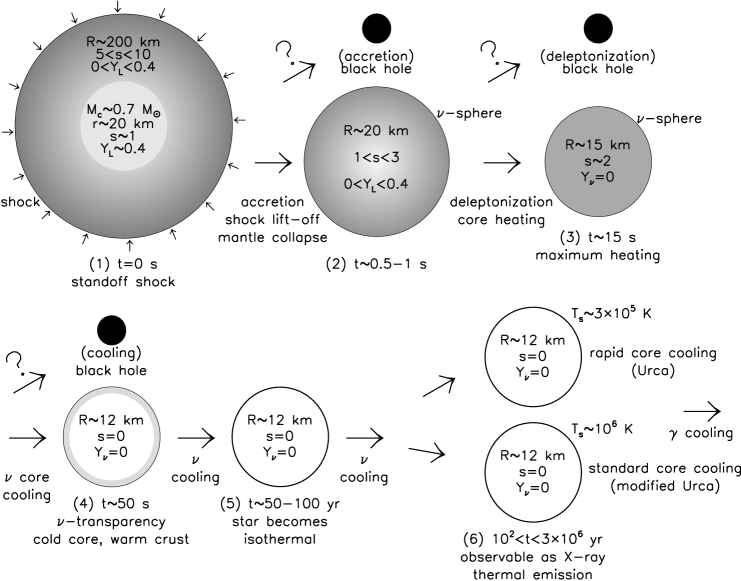
Figure 1.6: The main stages of the evolution of neutron stars [49]. Shading indicates approximate relative temperatures.

The evolution of protoneutron stars goes through several stages [47, 48, 49] as is shown in Fig. 1.6. During the supernova explosion, there goes a shock through the outer mantle of the protoneutron star. The outer mantle is of low density and high entropy, accretes matter and loses energy by $\beta$ decays and neutrino emission. The core has a mass of about 0.7 $\mathrm{M}_{\odot}$ in which neutrinos are trapped. The lepton to baryon fraction is $Y_{L}\simeq 0.4$. The whole protoneutron star in this first stage of evolution has an approximate radius of about 200 kilometers. After approximately five seconds, accretion becomes less important. The mantle collapses because of the loss of lepton pressure caused by deleptonization. In this stage of evolution, the lepton to baryon fraction is in the range $0<Y_{L}<0.4$, and the radius amounts to approximately 20 kilometers. If a lot of matter accretes onto the protoneutron star so that it exceeds its maximum mass then the protoneutron star collapses to a black hole. At approximately 15 seconds after the supernova explosion, the protoneutron star is dominated by neutrino diffusion causing deleptonization and heating of the protoneutron star. In this stage of evolution, the lepton to baryon fraction is $Y_{L}=0$, the radius of the protoneutron star is approximately 15 kilometers, and its temperature is heating up to 30 MeV $\lesssim T\lesssim$ 60 MeV. There is also the possibility of forming a black hole by deleptonization. Fifty seconds after the supernova explosion, the protoneutron star becomes transparent to neutrinos so that the inner part of the star cools down. But the crust remains warm because of its lower neutrino emissivity, $T\simeq 3\cdot 10^{6}$ K. After 50–100 years, also the crust cools down by neutrino emission and the star becomes isothermal. In later stages, the star cools down by direct URCA processes,

$$\mathrm{n}\longrightarrow\mathrm{p}+\mathrm{e}^{-}+\bar{\nu}_{\mathrm{e}}\;,\qquad\mathrm{p}+\mathrm{e}^{-}\longrightarrow\mathrm{n}+\nu_{\mathrm{e}}\;,$$ (1.37)

or modified URCA processes,

$$\mathrm{n}+\mathrm{n}\longrightarrow\mathrm{n}+\mathrm{p}+\mathrm{e}^{-}+\bar{\nu}_{\mathrm{e}}\;,\qquad\mathrm{n}+\mathrm{p}+\mathrm{e}^{-}\longrightarrow\mathrm{n}+\mathrm{n}+\nu_{\mathrm{e}}\;,$$ (1.38)

neutrino and photo emission. A cold neutron star has been formed.

1.4.1 Pulsars

Before neutron stars were discovered, theorists speculated about the existence of neutron stars. In 1932, Landau called them weird stars. In 1934, Baade and Zwicky realized that there is a connection between supernovae of type II and neutron stars. The first neutron star calculations were done by Tolman, Oppenheimer, and Volkoff in 1939 who created mass-radius diagrams of neutron stars [50]. Further work has been done by Wheeler et al. (1960–1966) and Pacini (1967).

In the summer of 1967 in Cambridge/England, Jocelyn Bell, a student of Anthony Hewish who got the Nobel prize in 1974, detected a neutron star as a pulsar for the first time. Neutron stars can be observed as pulsars which are pulsating sources of radiation because they can be identified by their very precise radio pulses. Pulsars possess a strong magnetic field of about 10¹² G in which highly energetic electrons gyrate and thereby produce synchroton radiation which is emitted at the magnetic poles of the pulsar, see Fig. 1.7. Usually, the rotation axis of a pulsar is inclined to the axis of the magnetic field. Thereby, the cone of the synchroton radiation can be detected only once in a rotation period of the pulsar. This is the pulsation phenomenon of pulsars which is also called the lighthouse effect.

From observations with radio telescopes one knows that pulsars have periods in the range of 1.6 milliseconds to several seconds. They rotate so fast because of angular-momentum conservation. In Sec. 1.3.1, it was mentioned that stars (gas balls) rotate. This rotation is kept during the life of the stars. When red super giants collapse to pulsars, the rotation velocity increases very much. The pulsar periods are very stable and therefore increase not much in time. The Crab pulsar for example has a rotation period of 33 milliseconds and this changes only about 0.036% per year. From the present pulsar period $P$ and its time derivative one is able to determine the characteristic age $\tau=P/\dot{P}$ of a pulsar. Because of the rapid rotation, a pulsar has an oblate shape and therefore is not exactly spherically symmetric. Observations like gravitational redshift measurements and mass determinations in binary systems as well as theoretical calculations show that the masses of neutron stars or pulsars, respectively, approximately amount to 1.5 $\mathrm{M}_{\odot}$, and that they have radii of about ten kilometers. Therefore such compressed, massive objects have an unbelievable mass density which is of about 10¹⁴ g/cm³. A further observation in pulsars are so-called glitches, sudden small jumps in the rotation period of pulsars. They are most probably caused by vortices and rearrangements in the crust of the pulsar. Because of that, it comes to a decrease of the angular momentum in the superfluid and an increase of the angular momentum in the crust [51]. Pulsars show proper motions which originate in so-called pulsar kicks. A possible explanation is that they are created if neutrinos emit asymmetrically during the supernova explosion which leads to a propulsion of the pulsar. Another observation in pulsars of binary systems are x-ray emissions and bursts: mass is transferred from companion stars onto the accretion disc of the pulsars. Because of the strong magnetic fields of the pulsars, matter from the accretion disc is diverted to the poles of the magnetic field. At this places, nuclear fusion processes are initiated, which emit x-rays.

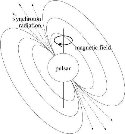
Figure 1.7: A schematic representation of a pulsar [7].

1.4.2 Structure of neutron stars

In Sec. 1.4, it was shown that neutron stars consist of neutrons because of inverse $\beta$ decays (1.36). This does not mean that neutron stars only consist of neutrons. For different mass densities, there are different phases of matter inside neutron stars, see Fig. 1.8.

Neutron stars consist of an atmosphere of electrons, nuclei, and atoms. Only a fraction of the electrons are bound to nuclei. The equation of state was calculated by Feynman, Metropolis, and Teller [52]. They found out that the nuclei in this regime, where the mass density $\rho\lesssim 10^{4}$ g/cm³, are mainly ⁵⁶Fe.

In neutron stars with temperatures above typically 100 eV, between the atmosphere and the solid crust a layer is present, where nuclei and electrons are in a liquid phase called the ocean [53].

One assumes complete ionization of the atoms, when the spacing between the nuclei becomes small compared to the Thomas-Fermi radius $r_{\mathrm{TF}}\simeq a_{0}Z^{-1/3}$ of an isolated neutral atom. In this equation, $a_{0}$ is the Bohr radius and $Z$ the charge number. The mass density approximately amounts to $\rho\simeq Am_{u}n_{N}$, where $A$ is the mass number, $m_{u}$ the atomic mass unit, and $n_{N}$ the number density of nuclei, which depends on the radius of a spherical nucleus whose volume is the average volume per nucleus [54], $\frac{4}{3}\pi r_{c}^{3}=1/n_{N}$. By combining the last three equations, one finds that the outer crust of cold neutron stars begins when $\rho\sim 10^{4}$ g/cm³ $\gg 3AZ$ g/cm³. This shell consists of nuclei and free electrons. The equation of state was originally calculated by Baym, Pethick, and Sutherland (BPS) [55] and improved in Refs. [56, 57] using up to date nuclear data. The BPS model is valid for zero temperature which is a good approximation for the crust of nonaccreting cold neutron stars. The outer crust of nonaccreting cold neutron stars contains nuclei and free electrons. The latter become relativistic above $\rho\sim 10^{7}$ g/cm³. The nuclei are arranged in a body-centered cubic (bcc) lattice. The contribution of the lattice has a small effect on the equation of state but it changes the equilibrium nucleus to a larger mass number and lowers the total energy of the system because it will minimize the Coulomb interaction energy of the nuclei. The latter are stabilized against $\beta$ decay by the filled electron sea. At $\rho\sim 10^{4}$ g/cm³, ⁵⁶Fe is the true ground state. With increasing mass density, it is not the true ground state any more because the nuclei capture electrons, emit neutrinos and become neutron richer. When the mass density $\rho\simeq 4.3\cdot 10^{11}$ g/cm³, the so-called neutron drip line is reached. Neutrons begin to drip out of the nuclei and become free. This happens because the equilibrium nuclei become more and more neutron-rich, and finally no more neutrons can be bound to nuclei. At the neutron drip point, the inner crust of neutron stars begins. At $\rho\simeq 2\cdot 10^{14}$ g/cm³ nuclei do not exist anymore, signalling the end of the neutron star crust.

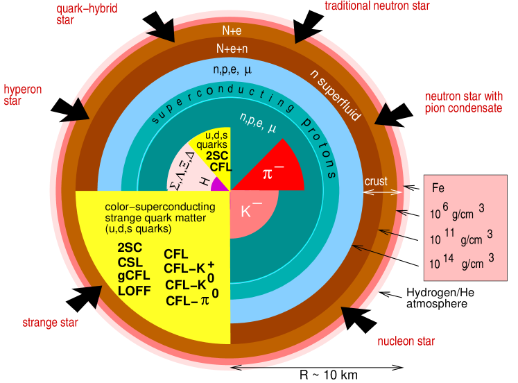
Figure 1.8: Cross-sections of neutron stars (schematic) [58]. Each sector shows another possible type of neutron stars.

The equation of state of the inner crust was calculated by Baym, Bethe, and Pethick [59] and another equation of state for this regime was derived by Negele and Vautherin [60]. Also a relativistic mean field model has been used to describe the density regime of the neutron star crust within the Thomas-Fermi approximation (see Ref. [61] and references therein). For higher densities, the nuclei disintegrate and their constituents, the protons and neutrons, become superfluid. Muons also begin to appear in these shells. The equation of state of this regime can be calculated by using non-relativistic many-body theories [62] or relativistic nuclear field theories [63, 64, 65, 66]. What kind of matter exists in the cores of neutron stars depends on their central densities. Neutron stars with lower central densities consist of protons, neutrons, electrons, and muons while others with larger central densities can consist of hyperons, a pion or kaon condensate. In neutron stars with huge central densities, $n\approx 10n_{0}$, even the protons, neutrons, and hyperons can disintegrate into their constituents: quarks which are deconfined. Such neutron stars contain a quark core [58] whose true ground state is strange quark matter [67] so that not only the light up and down quarks but also the strange quarks occur if their mass is low compared to the strange quark chemical potential. The remaining three quark flavors are too heavy to participate in the quark matter of neutron stars. Because of the dominant attractive interaction in the antitriplet channel, the true ground state of strange quark matter in the cores of neutron stars is color-superconducting strange quark matter [3, 9, 68, 69, 70, 71, 72, 73].

Figure 1.9: A schematic representation of the quark-hadron phase transition in neutron stars with a mass of about 1.4 $\mathrm{M}_{\odot}$ [74].

In nature, phase transitions can take place either through sharp boundaries between pure phases which are located next to each other or through mixed-phase regions. Thus, it does not necessarily mean that the phase transitions in neutron stars have to take place as sudden as represented in Fig. 1.8. In Fig. 1.9, one can see that the quark-hadron phase transition is not separated into two distinct shells but that there is a smooth transition from the hadronic phase into the quark phase. This transition goes in several stages, and by the effects of Coulomb forces and surface tensions, some interesting structures are formed. Quarks at first appear in a structure of drops in a shell under the pure hadronic phase in which the amount of hadrons exceeds the amount of quarks. With increasing density, quarks form a structure of rods, and finally a structure of slabs and are surrounded by hadronic matter. At higher density, the amount of quarks exceeds the amount of hadrons which form a structure of slabs. With increasing density, hadrons form a structure of rods, and finally a structure of drops that are surrounded by quark matter. Ultimately, the cores of neutron stars with huge central densities consist of pure quark matter.

1.4.3 Properties of neutron star matter

The matter in neutron stars is in its ground state. It is in nuclear equilibrium which means that the energy cannot be lowered by strong, weak, or electromagnetic interactions. When matter is in equilibrium concerning weak interactions, one calls it $\beta$-equilibrated matter or one says that matter is in $\beta$ equilibrium. It means that the reactions for (inverse) $\beta$ decay (1.36) or the reactions for weak interactions, respectively, are in equilibrium for all lepton families,

$$\mathrm{p}+\beta^{-}\longleftrightarrow\mathrm{n}+\nu_{\beta}\;.$$ (1.39)

In this equilibrated reaction, $\beta\equiv\left(e,\mu,\tau\right)$. The leptons are listed in Table 1.4. They are spin-$\frac{1}{2}$ particles, and therefore fermions.

Lepton	Mass [MeV]	$Q$ [e]	$g$
electron (e)	$0.51099906\pm 0.00000015$	$-1$	$2$
electron neutrino ($\nu_{e}$)	$<7.3\cdot 10^{-6}$	$0$	$1$
muon ($\mu$)	$105.658389\pm 0.000034$	$-1$	$2$
muon neutrino ($\nu_{\mu}$)	$<0.27$	$0$	$1$
$\tau$ lepton ($\tau$)	$1776.3\pm 2.4$	$-1$	$2$
$\tau$ neutrino ($\nu_{\tau}$)	$<31$	$0$	$1$

Table 1.4: The masses, electric charges, and degeneracy factors $g$ of the leptons [16]. The abbreviation for the respective lepton is shown in brackets. There also exists the corresponding antiparticle for each lepton with charge $-Q$. They are not shown here.

Since the quark flavor content of protons and neutrons is

$$\mathrm{p=(u,u,d)}\;,\qquad\mathrm{n=(u,d,d)}\;,$$ (1.40)

one can express the reaction (1.39) in terms of quark flavors,

$$\mathrm{u}+\beta^{-}\longleftrightarrow\mathrm{d}+\nu_{\beta}\;.$$ (1.41)

By weak interactions, also the transformation from up into strange quarks is possible,

$$\mathrm{u}+\beta^{-}\longleftrightarrow\mathrm{s}+\nu_{\beta}\;.$$ (1.42)

Neutrinos carry only lepton number. That is why the chemical potential of each neutrino family is equal to the chemical potential of each lepton family,

$$\mu_{\nu_{\beta}}\equiv\mu_{L_{\beta}}\;.$$ (1.43)

From the equilibrated reactions (1.41) and (1.42), one can directly write down the equation for the corresponding chemical potentials,

$$\mu_{u}+\mu_{\beta}=\mu_{d,s}+\mu_{L_{\beta}}\;,$$ (1.44)

where $\mu_{d,s}$ means that $\mu_{s}=\mu_{d}$, a fact that directly comes out of the equilibrated reactions (1.41) and (1.42). The last equation can be rewritten as

$$\mu_{u}=\mu_{d,s}+\mu_{Q}\;,$$ (1.45)

where

$$\mu_{Q}\equiv\mu_{L_{\beta}}-\mu_{\beta}$$ (1.46)

is the chemical potential of electric charge. This means that electrons, muons, and $\tau$ leptons carry both, lepton number and electric charge,

$$\mu_{\beta}=\mu_{L_{\beta}}-\mu_{Q}\;.$$ (1.47)

Because of the quark content of the neutron (1.40), one can define the baryon chemical potential

$$\mu_{B}\equiv 3\mu\equiv\mu_{n}=\mu_{u}+2\mu_{d}\;,$$ (1.48)

where $\mu$ is the quark chemical potential and $\mu_{n}$ the chemical potential of neutrons. This relation together with the fact that $\mu_{s}=\mu_{d}$ is used to solve the equation (1.45) for each quark flavor. One obtains

$$\mu_{ff^{\prime}}=\mu\delta_{ff^{\prime}}+\mu_{Q}Q_{ff^{\prime}}\;,$$ (1.49)

where

$$Q=\mathrm{diag}\left(\frac{2}{3},-\frac{1}{3},-\frac{1}{3}\right)$$ (1.50)

is the matrix of electric charge in flavor space.

With Eq. (1.49), one automatically satisfies $\beta$ equilibrium in normal quark matter where the color symmetry $[SU(3)_{c}]$ is not broken. This is not the case in color-superconducting quark matter. There, one has to know the quark chemical potential of each quark color and flavor. In order to satisfy $\beta$ equilibrium for each quark color and flavor, one starts with the equation for $\beta$ equilibrium for each quark flavor (1.49) and adds to it the terms for each color which consist of color chemical potentials and the generators of the $[SU(3)_{c}]$ group [75],

$$\mu_{ff^{\prime}}^{ii^{\prime}}=\left(\mu\delta_{ff^{\prime}}+\mu_{Q}Q_{ff^{\prime}}\right)\delta^{ii^{\prime}}+\delta_{ff^{\prime}}\sum_{c=1}^{8}\mu_{c}T_{c}^{ii^{\prime}}\;.$$ (1.51)

In this equation, the color indices $i$ and $i^{\prime}$ are superscripted while the flavor indices $f$ and $f^{\prime}$ are subscripted. But not all of the eight color chemical potentials are nonzero. This can be proven by calculating the tadpoles and was done for the 2SC phase in Ref. [76] where only a nonzero color chemical potential $\mu_{8}$ is present. I extended this calculation for the color-superconducting phases which I had to investigate for this thesis and got the result that there are nonzero color chemical potentials $\mu_{3}$ and $\mu_{8}$. Therefore, the chemical potential for each color and flavor can be simplified to

$$\mu_{ff^{\prime}}^{ii^{\prime}}=\left(\mu\delta_{ff^{\prime}}+\mu_{Q}Q_{ff^{\prime}}\right)\delta^{ii^{\prime}}+\,(\mu_{3}T_{3}^{ii^{\prime}}+\mu_{8}T_{8}^{ii^{\prime}})\,\delta_{ff^{\prime}}$$ (1.52)

for the purposes of this thesis. Later on, I omit the double color and flavor indices of the quark chemical potential matrix (1.52) and denote $\mu_{ff^{\prime}}^{ii^{\prime}}$ by $\mu_{f}^{i}$ because the quark chemical potential matrix (1.52) is diagonal in color-flavor space. Later on, also the double flavor indices of the matrix of electric charge (1.50) will be omitted because it is diagonal in flavor space, e.g. $Q_{ff^{\prime}}$ is denoted by $Q_{f}$. Also, the double color indices of the generators of the $[SU(3)_{c}]$ group, $T_{3}^{ii^{\prime}}$ and $T_{8}^{ii^{\prime}}$, can be omitted because they are diagonal in color space, e.g. $T_{3}^{ii^{\prime}}$ can be denoted by $T_{3}^{i}$, and $T_{8}^{ii^{\prime}}$ can be denoted by $T_{8}^{i}$.

Stars are bound by gravity and have to be electrically charge neutral, otherwise they would be unstable and explode because of repulsive Coulomb forces. The number density of electrically charged particles is given by

$$n_{Q}=\langle\psi^{\dagger}Q\psi\rangle-n_{e}-n_{\mu}-n_{\tau}\;,$$ (1.53)

where $\psi$ is the quark spinor, and $n_{e}$, $n_{\mu}$, and $n_{\tau}$ are the number densities of electrons, muons, and $\tau$ leptons, respectively. The electrical charge neutrality condition,

$$n_{Q}\equiv\frac{\partial p}{\partial\mu_{Q}}=0\;,$$ (1.54)

demands that the number density of electrically charged particles $n_{Q}$, which can be calculated by taking the derivative of the pressure $p$ with respect to the chemical potential of electric charge, is equal to zero.

Stars without color-superconducting quark matter are automatically color neutral because the $[SU(3)_{c}]$ color symmetry is not broken. This is not the case in color-superconducting quark matter. If stars consist of color-superconducting quark matter, then they have to be color neutral because on the one hand, one is not able to observe color charges in nature, on the other hand, stars will not be stable if they are not color neutral. In the following, I show that the color number densities $n_{3}$ and $n_{8}$ have to be equal to zero in order to fulfill color neutrality.

The spinor of quark colors is defined by

$$\psi=\left(\psi_{r},\psi_{g},\psi_{b}\right)^{T}\;.$$ (1.55)

Herewith, the number densities of quarks read,

$$n_{r}\equiv\langle\psi_{r}^{\dagger}\psi_{r}\rangle\;,\qquad n_{g}\equiv\langle\psi_{g}^{\dagger}\psi_{g}\rangle\;,\qquad n_{b}\equiv\langle\psi_{b}^{\dagger}\psi_{b}\rangle\;,$$ (1.56)

so that

$$n \equiv \langle\psi^{\dagger}\psi\rangle=n_{r}+n_{g}+n_{b}\;,$$ (1.57a)

$$n_{3} \equiv \langle\psi^{\dagger}T_{3}\psi\rangle=\textstyle\frac{1}{2}\displaystyle\left(n_{r}-n_{g}\right)\;,$$ (1.57b)

$$n_{8} \equiv \langle\psi^{\dagger}T_{8}\psi\rangle=\textstyle\frac{1}{2\sqrt{3}}\displaystyle\left(n_{r}+n_{g}-2n_{b}\right)\;.$$ (1.57c)

I only need to consider the color number densities $n_{3}$ and $n_{8}$ because there are only nonzero color chemical potentials $\mu_{3}$ and $\mu_{8}$ in the color-superconducting phases which I had to investigate for this thesis. In order to fulfill color neutrality, equal number densities of red, green, and blue quarks are necessary,

$$n_{r}=n_{g}=n_{b}\;.$$ (1.58)

By inserting this into Eqs. (1.57), one obtains the conditions for color neutrality,

$$n_{3}=n_{8}=0\;.$$ (1.59)

The color neutrality conditions

$$n_{3}\equiv\frac{\partial p}{\partial\mu_{3}}=0\;,\qquad n_{8}\equiv\frac{\partial p}{\partial\mu_{8}}=0\;,$$ (1.60)

demand that the number densities of color charges $n_{3}$ and $n_{8}$, which can be calculated by taking the derivative of the pressure $p$ with respect to the corresponding color chemical potential, are equal to zero.

In QCD, color neutrality is realized dynamically due to the generation of gluon condensates $\langle A_{0}^{3}\rangle\neq 0$ and $\langle A_{0}^{8}\rangle\neq 0$ [76, 77, 78]. The appearance of such condensates is equivalent to nonzero values of the corresponding color chemical potentials $\mu_{3}$ and $\mu_{8}$.

1.4.4 Toy models of neutral normal quark matter

In this thesis, I present the phase diagram of neutral quark matter. This will be done in Chapter 2. For a better understanding of the properties of neutral quark matter, it is advantageous to introduce some simple toy models. Therefore, some formulae of thermodynamics and statistical mechanics are needed [79, 80]. The pressure for non-interacting massive fermions and antifermions at nonzero temperature $T$ reads [81, 82],

$$p=\frac{gT}{2\pi^{2}}\int_{0}^{\infty}\mathrm{d}k\,k^{2}\left\{\ln\left[1+\exp\left(-\frac{E-\mu}{T}\right)\right]+\ln\left[1+\exp\left(-\frac{E+\mu}{T}\right)\right]\right\}\;,$$ (1.61)

where $g$ is the degeneracy factor, $k\equiv|\mathbf{k}|$ is the momentum, $E=\sqrt{k^{2}+m^{2}}$ is the relativistic total energy, $m$ is the mass, and $\mu$ is the chemical potential of the fermions. The first term corresponds to the pressure of fermions while the second one corresponds to the pressure of antifermions. By integration by parts, one obtains,

$$p=\frac{g}{6\pi^{2}}\int_{0}^{\infty}\mathrm{d}k\,\frac{k^{4}}{E}\left[n_{F}\left(\frac{E-\mu}{T}\right)+n_{F}\left(\frac{E+\mu}{T}\right)\right]\;,$$ (1.62)

where

$$n_{F}\left(x\right)\equiv\frac{1}{\mathrm{e}^{x}+1}\;,$$ (1.63)

is the Fermi-Dirac distribution function. At zero temperature, the Fermi-Dirac distribution function becomes a Heaviside function, cf. Eq. (1.1),

$$\lim_{T\rightarrow 0}n_{F}\left(\frac{x}{T}\right)=\theta\left(-x\right)\;,$$ (1.64)

so that one has to integrate from $k=0$ up to the Fermi momentum,

$$k_{F}\equiv\sqrt{\mu^{2}-m^{2}}\;.$$ (1.65)

Herewith, one obtains from Eq. (1.62) the pressure of non-interacting massive fermions for zero temperature,

$$p=\frac{g}{6\pi^{2}}\int_{0}^{k_{F}}\mathrm{d}k\,\frac{k^{4}}{E}\;.$$ (1.66)

Only the contribution from fermions survives. The pressure of non-interacting massive fermions for zero temperature can also be obtained by using the equation,

$$p=\frac{g}{2\pi^{2}}\int_{0}^{k_{F}}\mathrm{d}k\,k^{2}\left(\mu-E\right)\;.$$ (1.67)

This result can be calculated directly from the pressure (1.61) by using the relation,

$$\lim_{T\rightarrow 0}\ln\left[1+\exp\left(-\frac{x}{T}\right)\right]=-x\,\theta\left(-x\right)\;,$$ (1.68)

or by integration by parts of Eq. (1.66). The integrals in Eqs. (1.66) and (1.67) have an analytical solution,

$$p=\frac{g}{24\pi^{2}}\left[k_{F}\mu^{3}-\frac{5}{2}m^{2}k_{F}\mu-\frac{3}{2}m^{4}\ln\left(\frac{m}{k_{F}+\mu}\right)\right]\;,$$ (1.69)

while the integrals in Eqs. (1.61) and (1.62) can only be solved numerically. In the limit of vanishing mass, one obtains from Eq. (1.62) the pressure of non-interacting massless fermions and antifermions at nonzero temperature,

$$p=\frac{g}{24\pi^{2}}\left(\mu^{4}+2\pi^{2}\mu^{2}T^{2}+\frac{7}{15}\pi^{4}T^{4}\right)\;.$$ (1.70)

Details how to get this result are shown in Sec. B.1 in the Appendix. In the limit of zero mass and zero temperature, the pressure of fermions reads,

$$p=\frac{g}{24\pi^{2}}\mu^{4}\;.$$ (1.71)

The number density of non-interacting fermions can be obtained by

$$n=\frac{\partial p}{\partial\mu}\;,$$ (1.72)

which, in the case of massive fermions at nonzero temperature, leads to the result,

$$n=\frac{g}{2\pi^{2}}\int_{0}^{\infty}\mathrm{d}k\,k^{2}\left[n_{F}\left(\frac{E-\mu}{T}\right)-n_{F}\left(\frac{E+\mu}{T}\right)\right]\;.$$ (1.73)

The first term is the contribution of fermions while the second one is the contribution of antifermions. The integral can only be solved numerically, but in the case of zero temperature, one obtaines an analytical result by using Eq. (1.64),

$$n=\frac{g}{6\pi^{2}}k_{F}^{3}\;.$$ (1.74)

The number density of massless fermions and antifermions at nonzero temperature reads

$$n=\frac{g}{6\pi^{2}}\left(\mu^{3}+\pi^{2}\mu T^{2}\right)\;,$$ (1.75)

so that the number density of massless fermions at zero temperature is

$$n=\frac{g}{6\pi^{2}}\mu^{3}\;.$$ (1.76)

From these formulae of thermodynamics and statistical mechanics one is able to construct simple toy models for quark matter. In the following, I present toy models of non-interacting normal quark matter in neutron stars. Toy models for color-superconducting quark matter will be presented in Sec. 1.5.1. If a protoneutron star consists of normal quark matter, then one has to consider neutral $\beta$-equilibrated quark matter at nonzero temperature. Electrons and muons are present in quark matter in protoneutron stars in order to make them electrically neutral. Charm, bottom, and top quarks as well as $\tau$ leptons are too heavy so that they do not exist in the cores of compact stars where the quark chemical potential $\mu\simeq 500$ MeV. But in protoneutron stars, neutrinos are trapped. They can be treated as massless in good approximation. The pressure of a simple toy model of normal quark matter in protoneutron stars reads

$$p_{\mathrm{NQ}} = \frac{3T}{\pi^{2}}\sum_{f=u}^{s}\int_{0}^{\infty}\mathrm{d}k\,k^{2}\left\{\ln\left[1+\exp\left(-\frac{E_{f}-\mu_{f}}{T}\right)\right]+\ln\left[1+\exp\left(-\frac{E_{f}+\mu_{f}}{T}\right)\right]\right\}$$ (1.77)

$$+ \frac{T}{\pi^{2}}\sum_{\beta=e}^{\mu}\int_{0}^{\infty}\mathrm{d}k\,k^{2}\left\{\ln\left[1+\exp\left(-\frac{E_{\beta}-\mu_{\beta}}{T}\right)\right]+\ln\left[1+\exp\left(-\frac{E_{\beta}+\mu_{\beta}}{T}\right)\right]\right\}$$

$$+ \frac{1}{24\pi^{2}}\sum_{\beta=e}^{\mu}\left(\mu_{L_{\beta}}^{4}+2\pi^{2}\mu_{L_{\beta}}^{2}T^{2}+\frac{7}{15}\pi^{4}T^{4}\right)-B\;,$$

where the first line in this equation is the contribution of quarks, the second line is the contribution of electrons and muons, and the third line is the contribution of massless electron and muon neutrinos to the pressure. In the third line, also the bag pressure is subtracted. The relativistic energies of quarks, electrons, and muons are given by $E_{f}=(k^{2}+M_{f}^{2})^{1/2}$ and $E_{\beta}=(k^{2}+m_{\beta}^{2})^{1/2}$, where $M_{f}$ and $m_{\beta}$ are the masses of the quark flavors ($f=u,d,s$) and leptons ($\beta=e,\mu$). The chemical potentials of the quark flavors and the leptons are denoted by $\mu_{f}$ (1.49) or $\mu_{\beta}$, respectively, where

$$\mu_{\beta}\equiv\mu_{L_{\beta}}-\mu_{Q}\;,$$ (1.78)

cf. Eq. (1.46). Because of color symmetry and spin degeneracy, the degeneracy factor of the quark contribution to the pressure is $g=2N_{c}=6$. The degeneracy factor of electrons and muons is $g=2$ because of spin degeneracy. For neutrinos the spin is always opposite the momentum and this is referred to as left-handed, whereas the antineutrinos are always right-handed. That is why the degeneracy factor of neutrinos is $g=1$. The chemical potential of muon neutrinos can be set equal to zero which is a good approximation for matter in protoneutron stars. Electrical neutrality can be achieved by using Eq. (1.54),

$$n_{Q}\equiv\frac{\partial p_{\mathrm{NQ}}}{\partial\mu_{Q}}=\sum_{f=u}^{s}\frac{\partial p_{\mathrm{NQ}}}{\partial\mu_{f}}\frac{\partial\mu_{f}}{\partial\mu_{Q}}+\sum_{\beta=e}^{\mu}\frac{\partial p_{\mathrm{NQ}}}{\partial\mu_{\beta}}\frac{\partial\mu_{\beta}}{\partial\mu_{Q}}=\sum_{f=u}^{s}Q_{f}n_{f}-\sum_{\beta=e}^{\mu}n_{\beta}=0\;,$$ (1.79)

where

$$n_{f}=\frac{3}{\pi^{2}}\int_{0}^{\infty}\mathrm{d}k\,k^{2}\left[n_{F}\left(\frac{E_{f}-\mu_{f}}{T}\right)-n_{F}\left(\frac{E_{f}+\mu_{f}}{T}\right)\right]$$ (1.80)

is the net number density of each quark flavor, and

$$n_{\beta}=\frac{1}{\pi^{2}}\int_{0}^{\infty}\mathrm{d}k\,k^{2}\left[n_{F}\left(\frac{E_{\beta}-\mu_{\beta}}{T}\right)-n_{F}\left(\frac{E_{\beta}+\mu_{\beta}}{T}\right)\right]$$ (1.81)

is the number density of electrons or muons, respectively. As one expects, the condition for electrical neutrality of non-interacting normal quark matter in $\beta$ equilibrium (1.79) is of the form $\sum_{i}Q_{i}n_{i}=0$, where $Q_{i}$ is the electric charge of the particle species $i$ and $n_{i}$ its number density. In order to have neutral quark matter, for a given quark chemical potential $\mu$, the chemical potential of electric charge $\mu_{Q}$ has to be found by solving for it in Eq. (1.79).

A simple toy model for cold normal quark matter in neutron stars can be obtained by taking the limit $T\rightarrow 0$ in the above simple toy model for protoneutron stars. Also, neutrinos can be neglected because in cold neutron stars, they are not trapped any more. Therefore, the pressure of a simple toy model of cold normal quark matter in neutron stars reads

$$p_{\mathrm{NQ}}=\frac{1}{\pi^{2}}\sum_{f=u}^{s}\int_{0}^{k_{F_{f}}}\mathrm{d}k\,\frac{k^{4}}{E_{f}}+\frac{1}{3\pi^{2}}\sum_{\beta=e}^{\mu}\int_{0}^{k_{F_{\beta}}}\mathrm{d}k\,\frac{k^{4}}{E_{\beta}}\;,$$ (1.82)

where $k_{F_{f}}\equiv(\mu_{f}^{2}-M_{f}^{2})^{1/2}$ and $k_{F_{\beta}}\equiv(\mu_{\beta}^{2}-m_{\beta}^{2})^{1/2}$ are the Fermi momenta of the quark flavors $f$ and leptons $\beta$, respectively. Again, electrical neutrality can be achieved by solving Eq. (1.79) for the chemical potential $\mu_{Q}$ for a given quark chemical potential $\mu$. But for $T\rightarrow 0$, the expressions for the number density of each quark flavor and for each lepton respectively simplify to

$$n_{f}=\frac{k_{F_{f}}^{3}}{\pi^{2}}\;,\qquad n_{\beta}=\frac{k_{F_{\beta}}^{3}}{3\pi^{2}}\;.$$ (1.83)

In the limit of zero temperature, zero up and down quark masses, and massless electrons, and by neglecting the contribution of muons, one can solve Eq. (1.79) for the chemical potential of electric charge [83],

$$\mu_{Q}\simeq-\frac{M_{s}^{2}}{4\mu}\;,$$ (1.84)

where the Taylor expansion of the strange quark Fermi momentum,

$$k_{F_{s}}=\sqrt{\mu_{s}^{2}-M_{s}^{2}}\simeq\mu_{s}-\frac{M_{s}^{2}}{2\mu_{s}}\simeq\mu_{s}-\frac{M_{s}^{2}}{2\mu}\;,$$ (1.85)

is used, and terms which are of higher order are neglected because their contributions are small. If the contribution of the strange quarks is neglected, one obtains,

$$\mu_{Q}\simeq-\frac{\mu}{5}\;.$$ (1.86)

Inserting this into Eq. (1.49) and calculating the respective quark flavor number densities (1.83) leads to the result that there are nearly twice as many down quarks as up quarks. The simple results for the chemical potential of charge (1.84) and (1.86) are a good approximation for $\mu\gg M_{s}$ as one can see by comparing it with Fig. 5 in Ref. [8]. One also realizes that strange quarks help neutralizing quark matter and therefore less electrons are needed. For the ideal but unrealistic case of zero strange quark mass, no electrons are present in neutral normal quark matter.

1.5 Color superconductivity in neutron stars

From the statements made in Sec. 1.4.2, one can expect strange quark matter in the cores of neutron stars where the density is so large that deconfined quark matter is able to exist. Because of the dominant attractive interaction in the antitriplet channel, quarks form Cooper pairs. The typical temperatures inside (proto)neutron stars are so low that the diquark condensate is not melted. That is why one expects not (only) normal strange quark matter but even color-superconducting strange quark matter in the cores of neutron stars.

The color-superconducting gap affects the transport properties, e.g. conductivities and viscosities which have an influence on the cooling rates and on the rotation period of neutron stars. It also modifies the thermodynamic properties, e.g. the specific heat and the equation of state which have an influence on the mass-radius relation of color-superconducting neutron stars [9]. In Ref. [8], the effect of color superconductivity on the mass and the radius of compact stars made of pure quark matter is investigated. The authors confirmed the result of Ref. [86] that color superconductivity does not alter the mass and the radius of quark stars, if the diquark-coupling constant is chosen to reproduce vacuum properties such as the pion-decay constant. The reason is that color superconductivity in neutral quark matter has a tiny effect on the equation of state, cf. Figs. 5.9 and 5.10 in Ref. [7]. The color-superconducting gap has significant effects on the mass and radius of quark stars only if the diquark-coupling constant is artifically increased whereby the value of the gap itself artificially increases. For gaps on the order of 300 MeV, the mass and radius of quark stars are approximately twice as large as for normal-conducting quark stars so that such quark stars are of the same size and mass as ordinary neutron stars. Therefore, it is impossible to decide whether a compact star consists of normal conducting or color-superconducting quark matter, or simply of hadronic matter.

     

Figure 1.10: The low-energy part of the dispersion relations, i.e. the quasiparticle energies as a function of the quark momentum. Left panel: dispersion relations of quark quasiparticles in the 2SC phase (solid lines) and the normal quark phase (dashed lines). Right panel: dispersion relations of quark quasiparticles in the g2SC phase (solid lines) and the normal quark phase (dashed lines). The dispersion relation with the lowest energy in the g2SC phase shows a gapless mode [9, 84, 85]. The value of the averaged chemical potential of the up and down quarks which pair is denoted by $\bar{\mu}$ and one half of the difference of their chemical potentials is denoted by $\delta\mu$. In the massless case, the chemical potentials of the free up and down quarks are replaced by $\mu^{\pm}\equiv\bar{\mu}\pm[(\delta\mu)^{2}-\Delta^{2}]^{1/2}$.

In some cases, color superconductivity is accompanied by baryon superfluidity or the electromagnetic Meissner effect. Baryon superfluidity causes rotational vortices while the electromagnetic Meissner effect entails magnetic flux tubes in the cores of neutron stars.

At large strange quark masses, neutral two-flavor quark matter in $\beta$ equilibrium can have another rather unusual ground state called the gapless two-flavor color superconductor (g2SC) [84]. While the symmetry in the g2SC ground state is the same as that in the conventional 2SC phase, the spectrum of the fermionic quasiparticles is different, see Fig. 1.10. The g2SC phase appears at intermediate values of the diquark coupling constant while the 2SC phase appears in the regime of strong diquark coupling. Gapless modes are created if the mismatch between the Fermi momenta of the quarks which pair becomes large. In the case of the g2SC phase, $\delta\mu>\Delta$ where $\delta\mu\equiv\mu_{e}/2$. The existence of gapless color-superconducting phases was confirmed in Refs. [8, 87, 88], and generalized to nonzero temperatures in Refs. [85, 89]. It is also shown that a gapless CFL (gCFL) phase appears in neutral strange quark matter [90, 91]. But gapless color-superconducting quark phases are unstable in some regions of the phase diagram of neutral quark matter because of chromomagnetic instabilities [92] so that another phase will be the preferred state. Chromomagnetic instabilities occur even in regular color-superconducting quark phases. The author of Ref. [93] shows that chromomagnetic instabilities occur only at low temperatures in neutral color-superconducting quark matter. The author of Ref. [94] points out that the instabilities might be caused by using BCS theory in mean-field approximation, where phase fluctuations have been neglected. With the increase of the mismatch between the Fermi surfaces of paired fermions, phase fluctuations play more and more an important role, and soften the superconductor. Strong phase fluctuations will eventually quantum-disorder the superconducting state, and turn the system into a phase-decoherent pseudogap state. By using an effective theory of the CFL state, the author of Ref. [95] demonstrates that the chromomagnetic instability is resolved by the formation of an inhomogeneous meson condensate. The authors of Ref. [96] describe a new phase in neutral two-flavor quark matter within the framework of the Ginzburg-Landau approach, in which gluonic degrees of freedom play a crucial role. They call it a gluonic phase. In this phase, gluon condensates cure a chromomagnetic instability in the 2SC solution and lead to spontaneous breakdown of the color gauge symmetry, the $[U(1)_{\mathrm{em}}]$ and the rotational $SO(3)$ group. In other words, the gluonic phase describes an anisotropic medium in which color and electric superconductivity coexist. In Ref. [97], it was suggested that the chromomagnetic instability in gapless color-superconducting phases indicates the formation of the Larkin-Ovchinnikov-Fulde-Ferrell (LOFF) phase [98] which is discussed in Ref. [99] in the context of quark matter. Other possibilities could be the formation of a spin-one color-superconducting quark phase, a mixed phase, or a completely new state. The authors of Ref. [100] suggest that a mixed phase composed of the 2SC phase and the normal quark phase may be more favored if the surface tension is sufficiently small [101]. The authors of Ref. [102] suggest a single first-order phase transition between CFL and nuclear matter. Such a transition, in space, could take place either through a mixed phase region or at a single sharp interface with electron-free CFL and electron-rich nuclear matter in stable contact. The authors of Ref. [102] constructed a model for such an interface.

1.5.1 Toy models of neutral color-superconducting quark matter

In this subsection, I show some toy models for color-superconducting quark matter. In these toy models, which are valid for zero temperature, up and down quarks are treated as massless, and the strange quark mass is incorporated via a shift in the strange quark chemical potential which is a good approximation. Neutrinos are not present in cold quark matter in neutron stars so that $\mu_{e}\equiv-\mu_{Q}$. Also, muons are not taken into account in the following toy models but electrons which are treated as massless for simplicity. In the equations which satisfy the neutrality conditions of these toy models, terms of higher order will be neglected. The pressure of the toy model for color-superconducting quark matter in the 2SC phase reads [83],

$$p_{\mathrm{2SC}} = \frac{1}{\pi^{2}}\sum_{i=r}^{g}\sum_{f=u}^{d}\int_{0}^{\left(k_{F}\right)_{f}^{i}}\mathrm{d}k\,k^{2}\left(\mu_{f}^{i}-E_{f}\right)$$ (1.87)

$$+ \frac{1}{12\pi^{2}}\sum_{f=u}^{d}\left(\mu_{f}^{b}\right)^{4}+\frac{1}{3\pi^{2}}\sum_{i=r}^{b}\int_{0}^{\left(k_{F}\right)_{s}^{i}}\mathrm{d}k\,\frac{k^{4}}{E_{s}}$$

$$+ \frac{\mu_{e}^{4}}{12\pi^{2}}+\frac{\mu^{2}\Delta^{2}}{\pi^{2}}-B\;,$$

where the first line is the contribution of gapped quasiparticles, the second line is the contribution of free blue up and free blue down quarks as well as free strange quarks, and the third line is the contribution of massless electrons, the pressure correction due to the four gapped quasiparticles, and the bag pressure. The chemical potential for each quark color and flavor is given by Eq. (1.52), and their Fermi momenta by

$$\left(k_{F}\right)_{f}^{i}\equiv\sqrt{(\mu_{f}^{i})^{2}-M_{f}^{2}}\;.$$ (1.88)

Up and down quarks are treated as massless in this toy model, and the strange quark Fermi momenta for each color will be calculated by the simplified expression,

$$\left(k_{F}\right)_{s}^{i}=\sqrt{(\mu_{s}^{i})^{2}-M_{s}^{2}}\simeq\mu_{s}^{i}-\frac{M_{s}^{2}}{2\mu_{s}^{i}}\simeq\mu_{s}^{i}-\frac{M_{s}^{2}}{2\mu}\;,$$ (1.89)

as mentioned above. All quarks which pair have the same common (averaged) Fermi momenta,

$$k_{F}^{\mathrm{common}}\equiv k_{F_{1}}\equiv\left(k_{F}\right)_{u}^{r}=\left(k_{F}\right)_{d}^{g}=k_{F_{2}}\equiv\left(k_{F}\right)_{d}^{r}=\left(k_{F}\right)_{u}^{g}=\mu+\frac{1}{6}\mu_{Q}+\frac{1}{2\sqrt{3}}\mu_{8}\;.$$ (1.90)

In the 2SC phase, the Fermi momenta $k_{F_{1}}$ and $k_{F_{2}}$ are equal. Therefore, only one common Fermi momentum $k_{F}^{\mathrm{common}}$ is used. The neutrality conditions (1.54) and (1.60) require [83],

$$\mu_{Q}\simeq-\frac{M_{s}^{2}}{2\mu}\;,\qquad\mu_{3}=0\;,\qquad\mu_{8}\simeq 0\;.$$ (1.91)

In the case without strange quarks, one obtains

$$\mu_{Q}\simeq-\frac{\mu}{2}\;,\qquad\mu_{3}=0\;,\qquad\mu_{8}\simeq 0\;.$$ (1.92)

These approximations are in good agreement with the exact results for $\mu\gg M_{s}$, cf. Figs. 5 and 6 in Ref. [8]. In this toy model, the pressure difference of the 2SC phase to the normal quark phase reads [83]

$$\delta p_{\mathrm{2SC}}\simeq\frac{16\mu^{2}\Delta^{2}-M_{s}^{4}}{16\pi^{2}}$$ (1.93)

so that the 2SC phase is preferred to the normal quark phase when

$$\Delta>\frac{M_{s}^{2}}{4\mu}\;.$$ (1.94)

The pressure of the toy model for the CFL phase reads

$$p_{\mathrm{CFL}}=\frac{1}{\pi^{2}}\sum_{i=r}^{b}\sum_{f=u}^{s}\int_{0}^{\left(k_{F}\right)_{f}^{i}}\mathrm{d}k\,k^{2}\left(\mu_{f}^{i}-E_{f}\right)+\frac{\mu_{e}^{4}}{12\pi^{2}}+\frac{3\mu^{2}\Delta^{2}}{\pi^{2}}-B\;,$$ (1.95)

where the first term is the contribution of the nine gapped quarks, the second term is the contribution of electrons, the third term is the correction to the pressure due to the gap, and the fourth term is the bag pressure. As in the 2SC phase, the quarks which pair have the same Fermi momenta,

$$k_{F_{1}} \equiv \left(k_{F}\right)_{u}^{r}=\left(k_{F}\right)_{d}^{g}=\left(k_{F}\right)_{s}^{b}=\mu-\frac{M_{s}^{2}}{6\mu}\;,$$ (1.96a)

$$k_{F_{2}} \equiv \left(k_{F}\right)_{d}^{r}=\left(k_{F}\right)_{u}^{g}=\mu+\frac{1}{6}\mu_{Q}+\frac{1}{2\sqrt{3}}\mu_{8}\;,$$ (1.96b)

$$k_{F_{3}} \equiv \left(k_{F}\right)_{s}^{r}=\left(k_{F}\right)_{u}^{b}=\mu+\frac{1}{6}\mu_{Q}+\frac{1}{4}\mu_{3}-\frac{1}{4\sqrt{3}}\mu_{8}-\frac{M_{s}^{2}}{4\mu}\;,$$ (1.96c)

$$k_{F_{4}} \equiv \left(k_{F}\right)_{s}^{g}=\left(k_{F}\right)_{d}^{b}=\mu-\frac{1}{3}\mu_{Q}-\frac{1}{4}\mu_{3}-\frac{1}{4\sqrt{3}}\mu_{8}-\frac{M_{s}^{2}}{4\mu}\;.$$ (1.96d)

In the CFL phase, the neutrality condition for $\mu_{3}$, Eq. (1.60), requires that

$$\mu_{3}=-\mu_{Q}\;.$$ (1.97)

It is very useful to know that in the CFL phase the following relation is valid:

$$n_{Q}-n_{3}-\frac{1}{\sqrt{3}}n_{8}+n_{e}=0\;,$$ (1.98)

where $n_{e}$ is the number density of electrons. Because of the neutrality conditions, $n_{Q}$, $n_{3}$, and $n_{8}$ have to be equal to zero so that one concludes from Eq. (1.98) that also $n_{e}$ and with it $\mu_{e}$ have to be zero which is in agreement with the arguments made in Ref. [20]. It means that in the CFL phase there are neither electrons nor muons nor $\tau$ leptons allowed, otherwise the neutrality conditions will be violated. That is why one obtains the simple result

$$\mu_{Q}=\mu_{3}=0\;.$$ (1.99)

In order to satisfy the neutrality condition for $\mu_{8}$, Eq. (1.60), one gets,

$$\mu_{8}\simeq-\frac{M_{s}^{2}}{\sqrt{3}\mu}\;.$$ (1.100)

In this toy model, the pressure difference of the CFL phase to the normal quark phase reads [83, 102],

$$\delta p_{\mathrm{CFL}}\simeq\frac{48\mu^{2}\Delta^{2}-3M_{s}^{4}}{16\pi^{2}}$$ (1.101)

so that the CFL phase is preferred to the normal quark phase when

$$\Delta>\frac{M_{s}^{2}}{4\mu}\;.$$ (1.102)

This is the same requirement as for the 2SC phase, and because the pressure difference of the CFL phase to normal quark matter is three times larger than the pressure difference of the 2SC phase to normal quark matter, the authors of Ref. [83] claim that the 2SC phase is absent and the CFL phase is the preferred state in compact stars. In Chapter 2, I shall show that this statement is not correct in general so that these simple toy models cannot replace a thorough analysis of the preferred quark phases by an NJL model [14, 103, 104, 105, 106] for example. That is why it is so important to construct the phase diagram of neutral quark matter with a more precise model which is done in Chapter 2.

Chapter 2 The phase diagram of neutral quark matter

At sufficiently high densities and sufficiently low temperatures quark matter is a color superconductor [10, 11, 12]. This conclusion follows naturally from arguments similar to those employed in the case of ordinary low-temperature superconductivity in metals and alloys [13]. Of course, the case of quark matter is more complicated because quarks, unlike electrons, come in various flavors (e.g., up, down, and strange) and carry non-Abelian color charges. This phenomenon was studied in detail by various authors [15, 18, 19, 32, 33, 35, 36, 99, 107, 108, 109]. Many different phases were discovered, and recent studies [84, 85, 87, 88, 89, 90, 91, 110, 111, 112, 113, 114, 115, 116, 117, 118, 119] show that even more new phases exist. (For reviews and lectures on color superconductivity see Refs. [3, 9, 68, 69, 70, 71, 72, 73].)

In nature, the most likely place where color superconductivity may occur is the interior of neutron stars. Therefore, it is of great importance to study the phases of dense matter under the conditions that are typical for the interior of stars. For example, one should appreciate that matter in the bulk of a star is neutral and $\beta$-equilibrated. By making use of rather general arguments, it was suggested in Ref. [83] that such conditions favor the CFL phase and disfavor the 2SC phase. In trying to refine the validity of this conclusion, it was recently realized that, depending on the value of the constituent (medium modified) strange quark mass, the ground state of neutral and $\beta$-equilibrated dense quark matter may be different from the CFL phase. In particular, the g2SC phase [84, 85] is likely to be the ground state in the case of a large strange quark mass. On the other hand, in the case of a moderately large strange quark mass, the CFL and gCFL phases [90] are favored. At nonzero temperature, $T\neq 0$, some other phases were proposed as well [111].

I note that the analysis in this thesis is restricted to locally neutral phases only. This automatically excludes, for example, crystalline [99] and mixed [101, 100, 120] phases. Also, in the mean field approximation utilized here, I cannot get any phases with meson condensates [28, 29, 30].

In this chapter, I present the phase diagram of neutral quark matter. In Sec. 2.1, I show the phase diagram of massless neutral three-flavor quark matter. In Sec. 2.2, quark masses are treated self-consistently within the framework of a three-flavor NJL model [106], and the phase diagram with a self-consistent treatment of quark masses is presented. In Sec. 2.3, this NJL model is extended to nonzero neutrino chemical potentials, and the influence of neutrinos on the phase diagram is discussed.

I use the following conventions: I calculate in natural units, $\hbar=c=k_{B}=1$, and utilize the Dirac definition of the $\gamma$-matrices which are shown in Sec. A.2 in the Appendix. Latin indices run from one to three while Greek indices run from zero to three. Four-vectors are denoted by capital Latin letters while three-vectors are written in the bold upright font. The space-time vector is defined as $X^{\mu}=\left(x^{0},x^{1},x^{2},x^{3}\right)=\left(t,\mathbf{x}\right)$, the four-momentum vector is denoted as $K^{\mu}=\left(k^{0},\mathbf{k}\right)$, and the metric tensor is given by $g_{\mu\nu}=\mathrm{diag}\left(1,-1,-1,-1\right)$. Absolute values of vectors are denoted by italic Latin letters, e.g. $k=|\mathbf{k}|$. The direction of a vector is indicated by the hat symbol, e.g. $\hat{\mathbf{k}}=\mathbf{k}/k$. I use the imaginary-time formalism, i.e., the space-time integration is defined as $\int_{X}=\int_{0}^{1/T}\mathrm{d}\tau\int_{V}\mathrm{d}^{3}\mathbf{x}$, where $\tau$ is the Euclidean time coordinate and $V$ the three-volume of the system. The delta function is defined as $\delta^{\left(4\right)}\left(X-Y\right)\equiv\delta\left(\tau_{X}-\tau_{Y}\right)\delta^{\left(3\right)}\left(\mathbf{x}-\mathbf{y}\right)$. Energy-momentum sums are written as: $T/V\sum_{K}=T\sum_{n}\int\mathrm{d}^{3}\mathbf{k}/(2\pi^{3})=T/(2\pi^{2})\sum_{n}\int\mathrm{d}k\,k^{2}$, where the sum runs over the Matsubara frequencies $\omega_{n}=2n\pi T\equiv ik_{0}$ for bosons and $\omega_{n}=\left(2n+1\right)\pi T\equiv ik_{0}$ for fermions, respectively.

2.1 The phase diagram of massless quarks

In this section, I study the phase diagram of massless neutral three-flavor quark matter at zero and nonzero temperature as a function of the strange quark mass as well as a function of the quark chemical potential. I start with the QCD Lagrangian density in order to derive the QCD grand partition function. Then, the Cornwall-Jackiw-Tomboulis (CJT) formalism [121] is used to calculate the QCD effective action. The gluon-exchange interaction between quarks is approximated by a point-like four-fermion coupling. From the effective action of quarks, I derive the pressure of color-superconducting quark matter. In order to allow for the most general ground state, I employ a nine-parameter ansatz for the gap matrix [110]. The effects of the strange quark mass are incorporated by a shift of the chemical potential of strange quarks, $\mu^{i}_{s}\rightarrow\mu^{i}_{s}-m_{s}^{2}/(2\mu)$, where $i=r,g,b$ is the color index, $m_{s}$ is the strange quark mass, and $\mu$ is the quark chemical potential. This shift reflects the reduction of the Fermi momenta of strange quarks due to their mass. Such an approach is certainly reliable at small values of the strange quark mass. I assume that it is also qualitatively correct at large values of the strange quark mass. In order to draw the phase diagram of massless neutral three-flavor quark matter, I solve nine gap equations together with the conditions of electric and color charge neutrality.

2.1.1 Quantum chromodynamics

The QCD Lagrangian density is given by

$$\mathcal{L}=\bar{\psi}\left(iD\hbox to0.0pt{\hss$\diagup$}-\hat{m}\right)\psi-\frac{1}{4}F_{\mu\nu}^{a}F_{a}^{\mu\nu}+\mathcal{L}_{\mathrm{gauge}}\;.$$ (2.1)

For $N_{c}$ colors and $N_{f}$ flavors, $\psi$ is the $4N_{c}N_{f}$-dimensional spinor of quark fields, $\bar{\psi}\equiv\psi^{\dagger}\gamma_{0}$ is the Dirac conjugate spinor, $D\hbox to0.0pt{\hss$\diagup$}\equiv\gamma^{\mu}D_{\mu}$, where $\gamma^{\mu}$ are the Dirac matrices, and $\hat{m}$ is the quark-mass matrix. The covariant derivative is defined as

$$D_{\mu}\equiv\partial_{\mu}-igA_{\mu}^{a}T_{a}\;,$$ (2.2)

where $g$ is the strong-coupling constant, $A_{\mu}^{a}$ are the gluon fields, and $T_{a}$ are the generators of the $[SU(N_{c})_{c}]$ group. The gluon field-strength tensor is defined as

$$F_{a}^{\mu\nu}=\partial^{\mu}A_{a}^{\nu}-\partial^{\nu}A_{a}^{\mu}+gf_{abc}A_{b}^{\mu}A_{c}^{\nu}\;,$$ (2.3)

where $f_{abc}$ are the structure constants of the $[SU(N_{c})_{c}]$ group. The first term in the QCD Lagrangian density (2.1) corresponds to interacting quarks while the second one corresponds to the gluons. The term $\mathcal{L}_{\mathrm{gauge}}$ comprises gauge fixing terms and the contribution from Faddeev-Popov ghosts. Up to irrelevant constants, the grand partition function of QCD is given by [122, 123]

$$\mathcal{Z}=\int\mathcal{D}\bar{\psi}\mathcal{D}\psi\mathcal{D}A_{\mu}^{a}\exp\left\{I\left[\bar{\psi},\psi,A\right]\right\}\;,$$ (2.4)

where

$$I\left[\bar{\psi},\psi,A\right]=\int_{X}\left(\mathcal{L}+\mu\mathcal{N}+\mu_{Q}\mathcal{N}_{Q}+\mu_{a}\mathcal{N}_{a}\right)\;,$$ (2.5)

is the QCD action. The conserved quantities,

$$\mathcal{N}\equiv\bar{\psi}\gamma_{0}\psi\;,\qquad\mathcal{N}_{Q}\equiv\bar{\psi}\gamma_{0}Q\psi\;,\qquad\mathcal{N}_{a}\equiv\bar{\psi}\gamma_{0}T_{a}\psi\;,$$ (2.6)

are the quark number density operator, the operator of electric charge density of the quarks, and the operators of color charge densities of the quarks, respectively. The QCD action can be split into the part of interacting quarks, into the part of gluons, and into the part of gauge fixing terms and Faddeev-Popov ghosts,

$$I\left[\bar{\psi},\psi,A\right]=I_{\psi_{\mathrm{int}}}\left[\bar{\psi},\psi,A\right]+I_{A}\left[A\right]+I_{\mathrm{gauge}}\left[A\right]\;,$$ (2.7)

where

$$I_{\psi_{\mathrm{int}}}\left[\bar{\psi},\psi,A\right] = \int_{X,Y}\bar{\psi}\left(X\right)[\mathcal{G}_{0}^{+}]^{-1}\left(X,Y\right)\psi\left(Y\right)\;,$$ (2.8a)

$$I_{A}\left[A\right] = -\frac{1}{4}\int_{X}F_{\mu\nu}^{a}\left(X\right)F_{a}^{\mu\nu}\left(X\right)\;,$$ (2.8b)

$$I_{\mathrm{gauge}}\left[A\right] = \int_{X}\mathcal{L}_{\mathrm{gauge}}\;.$$ (2.8c)

The inverse tree-level propagator for quarks and charge-conjugate quarks, respectively, is given by

$${[\mathcal{G}_{0}^{+}]}{}^{-1}\left(X,Y\right) \equiv \,(iD\hbox to0.0pt{\hss$\diagup$}_{X}+\hat{\mu}\gamma_{0}-\hat{m})\,\delta^{\left(4\right)}\left(X-Y\right)\;,$$ (2.9a)

$${[\mathcal{G}_{0}^{-}]}{}^{-1}\left(X,Y\right) \equiv \,(iD\hbox to0.0pt{\hss$\diagup$}_{X}^{C}-\hat{\mu}\gamma_{0}-\hat{m})\,\delta^{\left(4\right)}\left(X-Y\right)\;,$$ (2.9b)

see Sec. B.2 in the Appendix. The matrix of quark chemical potentials is denoted by $\hat{\mu}$ and is defined by Eq. (1.51). The covariant derivative in the inverse tree-level propagator of quarks is given by Eq. (2.2) while the charge-conjugate covariant derivative in the inverse tree-level propagator of charge-conjugate quarks reads,

$$D\hbox to0.0pt{\hss$\diagup$}_{\mu}^{C}=\partial_{\mu}+igA_{\mu}^{a}T_{a}^{T}\;.$$ (2.10)

By using the charge-conjugate spinors (A.14) and by introducing the Nambu-Gorkov basis with the $2\cdot 4N_{c}N_{f}$-dimensional quark spinors,

$$\bar{\Psi}\equiv\left(\bar{\psi},\bar{\psi}_{C}\right)\;,\qquad\Psi\equiv\left(\begin{array}[]{c}\psi\\ \psi_{C}\end{array}\right)\;,$$ (2.11)

one can rewrite the QCD action of interacting quarks,

$$I_{\psi_{\mathrm{int}}}\left[\bar{\Psi},\Psi,A\right]=\frac{1}{2}\int_{X,Y}\bar{\Psi}\left(X\right)\mathcal{S}_{0}^{-1}\left(X,Y\right)\Psi\left(Y\right)\;,$$ (2.12)

where

$$\mathcal{S}_{0}^{-1}\equiv\left(\begin{array}[]{cc}[\mathcal{G}_{0}^{+}]^{-1}&0\\ 0&[\mathcal{G}_{0}^{-}]^{-1}\end{array}\right)$$ (2.13)

is the inverse tree-level propagator for Nambu-Gorkov quarks.

By adding a bilocal source term to the QCD action (2.7), one obtains [3, 37],

$$I\left[\bar{\Psi},\Psi,A,\mathcal{K}\right]\equiv I\left[\bar{\Psi},\Psi,A\right]+\frac{1}{2}\int_{X,Y}\bar{\Psi}\left(X\right)\mathcal{K}\left(X,Y\right)\Psi\left(Y\right)\;,$$ (2.14)

where

$$\mathcal{K}\equiv\left(\begin{array}[]{cc}\sigma^{+}&\varphi^{-}\\ \varphi^{+}&\sigma^{-}\end{array}\right)\;.$$ (2.15)

The four entries of $\mathcal{K}$ are not independent. Due to charge-conjugation invariance of the action, $\sigma^{-}\equiv C\left(\sigma^{+}\right)^{T}C^{-1}$, and since the action has to be real-valued, $\varphi^{-}\equiv\gamma_{0}\left(\varphi^{+}\right)^{\dagger}\gamma_{0}$. In the presence of an external source $\mathcal{K}$, the grand partition function of QCD, up to irrelevant constants, reads,

$$\mathcal{Z}\left[\mathcal{K}\right]=\int\mathcal{D}\bar{\Psi}\mathcal{D}\Psi\mathcal{D}A_{\mu}^{a}\exp\left\{I\left[\bar{\Psi},\Psi,A,\mathcal{K}\right]\right\}\;.$$ (2.16)

The QCD effective action can be derived from the grand partition function of QCD (2.16) by using the CJT formalism [3, 8, 37, 121, 124, 125, 126],

$$\Gamma\left[\bar{\Psi},\Psi,A,\mathcal{S},\mathcal{D}\right] = I\left[\bar{\Psi},\Psi,A\right]-\frac{1}{2}\mathrm{Tr}\ln\mathcal{D}^{-1}-\frac{1}{2}\mathrm{Tr}\left(\mathcal{D}_{0}^{-1}\mathcal{D}-1\right)$$ (2.17)

$$+ \frac{1}{2}\mathrm{Tr}\ln\mathcal{S}^{-1}+\frac{1}{2}\mathrm{Tr}\left(\mathcal{S}_{0}^{-1}\mathcal{S}-1\right)+\Gamma_{2}\left[\bar{\Psi},\Psi,A,\mathcal{S},\mathcal{D}\right]\;.$$

The quantities $\mathcal{D}$ and $\mathcal{S}$ are the gluon and quark propagator, respectively. The inverse tree-level quark propagator $\mathcal{S}_{0}^{-1}$ was introduced in Eq. (2.13). Correspondingly, $\mathcal{D}_{0}^{-1}$ is the inverse tree-level gluon propagator. The traces run over space-time, Nambu-Gorkov, color-flavor, and Dirac indices. The factor $\frac{1}{2}$ in front of the fermionic one-loop terms compensates the doubling of degrees of freedom in the Nambu-Gorkov basis. The functional $\Gamma_{2}$ is the sum of all two-particle irreducible (2PI) diagrams. It is impossible to evaluate all 2PI diagrams exactly. However, the advantage of the QCD effective action (2.17) is that truncating the sum $\Gamma_{2}$ after a finite number of terms still provides a well-defined many-body approximation. Later on, the gluon-exchange interaction between quarks is approximated by a point-like four-fermion coupling. This effectively removes dynamical gluon degrees of freedom, such that one does not need to worry about gauge fixing or possible ghost degrees of freedom. Therefore, the latter are already omitted in Eq. (2.17). The stationary points of the effective action (2.17) determine the expectation values of the one- and two-point functions,

$$\frac{\delta\Gamma}{\delta\bar{\Psi}}=0\;,\qquad\frac{\delta\Gamma}{\delta\Psi}=0\;,\qquad\frac{\delta\Gamma}{\delta A_{\mu}^{a}}=0\;,\qquad\frac{\delta\Gamma}{\delta\mathcal{D}}=0\;,\qquad\frac{\delta\Gamma}{\delta\mathcal{S}}=0\;.$$ (2.18)

The first two equations yield the Dirac equation for the quark fields $\Psi$ and $\bar{\Psi}$ in the presence of the gluon field $A_{\mu}^{a}$. The third equation is the Yang-Mills equation for the gluon field,

$$D_{\nu}^{ab}F^{\nu\mu}_{b}\left(X\right)=\frac{\delta}{\delta A_{\mu}^{a}\left(X\right)}\left[\frac{1}{2}\mathrm{Tr}\left(\mathcal{D}_{0}^{-1}\mathcal{D}-\mathcal{S}_{0}^{-1}\mathcal{S}\right)-\Gamma_{2}\right]\;,$$ (2.19)

where $D_{\nu}^{ab}=\partial_{\nu}\delta^{ab}-gf^{abc}A_{\nu}^{c}(X)$ is the covariant derivative in the adjoint representation. The first two terms on the right-hand side are the contributions from gluon and fermion tadpoles [76].

The functional derivative with respect to $A_{\mu}^{a}$ acting on the trace is nontrivial because of the dependence of the inverse tree-level propagators $\mathcal{D}_{0}^{-1}$ and $\mathcal{S}_{0}^{-1}$ on the gluon field, cf. Eq. (2.13). The last term is nonzero if $\Gamma_{2}$ contains 2PI diagrams with an explicit dependence on $A_{\mu}^{a}$. As shown in Ref. [76], the solution of the Yang-Mills equation in the 2SC phase is a constant background field $A_{\mu}^{a}\sim g_{\mu 0}\delta^{a8}$. This background field acts like a color chemical potential $\mu_{8}$ and provides the color-charge neutrality of the 2SC phase [76]. In this manner, also the color chemical potential $\mu_{3}$ is present in three-flavor color superconductors where the color chemical potentials $\mu_{3}$ and $\mu_{8}$ ensure color neutrality. Later on, I shall remove the gluon degrees of freedom by approximating the non-local gluon exchange with a point-like four-fermion coupling. The constant background field $A_{\mu}^{a}$ then disappears from the treatment, and the color chemical potentials $\mu_{3}$ and $\mu_{8}$ assume the role of the background field to ensure color neutrality.

The fourth equation (2.18) is the Dyson-Schwinger equation for the gluon propagator,

$${\mathcal{D}^{-1}}_{ab}^{\mu\nu}\left(X,Y\right)={\mathcal{D}_{0}^{-1}}_{ab}^{\mu\nu}\left(X,Y\right)+\Pi_{ab}^{\mu\nu}\left(X,Y\right)\;,$$ (2.20)

where

$$\Pi_{ab}^{\mu\nu}\left(X,Y\right)=-2\,\frac{\delta\Gamma_{2}}{\delta\mathcal{D}_{ba}^{\nu\mu}\left(Y,X\right)}$$ (2.21)

is the gluon self-energy. Since I shall approximate the gluon exchange by a four-fermion coupling, I do not need to solve the Dyson-Schwinger equation for the gluon propagator.

The fifth equation (2.18) is the Dyson-Schwinger equation for the quark propagator,

$$\mathcal{S}^{-1}\left(X,Y\right)=\mathcal{S}_{0}^{-1}\left(X,Y\right)+\Sigma\left(X,Y\right)\;,$$ (2.22)

where

$$\Sigma\left(X,Y\right)=2\,\frac{\delta\Gamma_{2}}{\delta\mathcal{S}\left(Y,X\right)}$$ (2.23)

is the quark self-energy. According to their definition, the self-energies (2.21) and (2.23) are obtained from the set of 2PI diagrams by opening one internal line. The quark self-energy is a $2\times 2$-matrix in Nambu-Gorkov space,

$$\Sigma=\left(\begin{array}[]{cc}\Sigma^{+}&\Phi^{-}\\ \Phi^{+}&\Sigma^{-}\end{array}\right)\;,$$ (2.24)

where the quantities $\Sigma^{\pm}$ are the regular self-energies, and $\Phi^{\pm}$ are the anomalous self-energies. For $\Phi^{\pm}$, also the term gap matrices is used. The gap matrices in connection with the quark self-energy (2.23) yield the so-called gap equations. By solving these gap equations, one obtains the gap parameters. In space-time, $\Sigma^{+}\left(X,Y\right)$ $\left[\Sigma^{-}\left(X,Y\right)\right]$ has a quark [charge-conjugate quark] entering at $X$ and another quark [charge-conjugate quark] emerging at $Y$. The anomalous self-energies have to be interpreted as follows: a quark [charge-conjugate quark] enters $\Phi^{+}\left(X,Y\right)$ $\left[\Phi^{-}\left(X,Y\right)\right]$ at $X$ and, in contrast to the regular self-energies, here, a charge-conjugate quark [an ordinary quark] emerges at $Y$. This is typical for systems with a fermion-fermion condensate in the ground state [127]. The self-energies $\Phi^{\pm}$ symbolize this condensate. This is why the crucial quantities regarding color superconductivity are the gap matrices $\Phi^{\pm}$. A nonzero value of $\Phi^{\pm}$ is equivalent to Cooper pairing, or, in other words, to a nonvanishing diquark expectation value. The self-energies in Eq. (2.24) are related in the same way as the bilocal sources in Eq. (2.15),

$$\Sigma^{-}\equiv C\left(\Sigma^{+}\right)^{T}C^{-1}\;,\qquad\Phi^{-}\equiv\gamma_{0}\left(\Phi^{+}\right)^{\dagger}\gamma_{0}\;.$$ (2.25)

The quark propagator in Nambu-Gorkov space can be determined from the Dyson-Schwinger equation (2.22), see Sec. B.3 in the Appendix,

$$\mathcal{S}=\left(\begin{array}[]{cc}\mathcal{G}^{+}&\Xi^{-}\\ \Xi^{+}&\mathcal{G}^{-}\end{array}\right)\;,$$ (2.26)

where

$$\mathcal{G}^{\pm}=\left\{[\mathcal{G}_{0}^{\pm}]^{-1}+\Sigma^{\pm}-\Phi^{\mp}\left([\mathcal{G}_{0}^{\mp}]^{-1}+\Sigma^{\mp}\right)^{-1}\Phi^{\pm}\right\}^{-1}\;,$$ (2.27)

is the propagator for quasiquarks or charge-conjugate quasiquarks, respectively, and

$$\Xi^{\pm}=-\left([\mathcal{G}_{0}^{\mp}]^{-1}+\Sigma^{\mp}\right)^{-1}\Phi^{\pm}\mathcal{G}^{\pm}=-\,\mathcal{G}^{\mp}\Phi^{\pm}\left([\mathcal{G}_{0}^{\pm}]^{-1}+\Sigma^{\pm}\right)^{-1}\;,$$ (2.28)

are the anomalous propagators. These anomalous propagators are typical for superconducting systems [127] and account for the possibility that in the presence of a Cooper-pair condensate, symbolized by $\Phi^{\pm}$, a fermion can always be absorbed in the condensate, while its charge-conjugate counterpart is emitted from the condensate and continues to propagate.

The QCD pressure is, up to a prefactor $T/V$, equal to the QCD effective action (2.17) determined at the stationary points (2.18) which is denoted by $\Gamma^{*}$,

$$p=\frac{T}{V}\Gamma^{*}\;,$$ (2.29)

where $T$ is the temperature and $V$ the volume of the system.

2.1.2 The effective action of quarks

In this section, I investigate the phase diagram of massless neutral three-flavor quark matter. The quark spinor has the following color-flavor structure:

$$\psi=\left(\psi_{u}^{r},\psi_{d}^{r},\psi_{s}^{r},\psi_{u}^{g},\psi_{d}^{g},\psi_{s}^{g},\psi_{u}^{b},\psi_{d}^{b},\psi_{s}^{b}\right)^{T}\;.$$ (2.30)

Since I approximate the gluon-exchange interaction between quarks by a point-like four-fermion coupling, I only need to consider the contributions of quarks to the QCD effective action (2.17),

$$\Gamma\left[S\right]=\frac{1}{2}\mathrm{Tr}\ln S^{-1}+\frac{1}{2}\mathrm{Tr}\left(S_{0}^{-1}S-1\right)+\Gamma_{2}\left[S\right]\;.$$ (2.31)

Here, the tree-level quark propagator $\mathcal{S}_{0}^{-1}$ (2.13), which occurs in the QCD effective action (2.17), is replaced by the quark propagator,

$$S_{0}^{-1}\equiv\left(\begin{array}[]{cc}[G_{0}^{+}]^{-1}&0\\ 0&[G_{0}^{-}]^{-1}\end{array}\right)\;,$$ (2.32)

where

$${[G_{0}^{\pm}]}{}^{-1}\left(X,Y\right)\equiv\,(i\partial\hbox to0.0pt{\hss$\diagup$\kern-2.0pt}_{X}\pm\hat{\mu}\gamma_{0})\,\delta^{\left(4\right)}\left(X-Y\right)\;,$$ (2.33)

is the massless inverse Dirac propagator for quarks and charge-conjugate quarks, respectively, in which the constant background field $A_{\mu}^{a}$ disappears from the treatment, and the color chemical potentials $\mu_{3}$ and $\mu_{8}$ assume the role of the background field to ensure color neutrality. The quark chemical potential matrix in color-flavor space is defined as

$$\hat{\mu}=\mathrm{diag}\left(\mu_{u}^{r},\mu_{d}^{r},\mu_{s}^{r},\mu_{u}^{g},\mu_{d}^{g},\mu_{s}^{g},\mu_{u}^{b},\mu_{d}^{b},\mu_{s}^{b}\right)\;,$$ (2.34)

where the chemical potential of each quark is given by Eq. (1.52) because quark matter inside neutron stars is in $\beta$ equilibrium.

Since I shall present the phase diagram of massless neutral three-flavor quark matter in this section, the mass term of the inverse Dirac propagators (2.33) is omitted. At sufficiently large quark chemical potential, there is no need to take into account the small up and down quark masses because the dynamical effect of such masses around the quark Fermi surfaces is negligible. Of course, the situation with the strange quark is different because its mass is not very small as compared to the quark chemical potential $\mu$. The most important effect of a nonzero strange quark mass is, however, a shift of the strange quark chemical potential due to the reduction of the Fermi momentum,

$$\left(k_{F}\right)_{s}^{i}=\sqrt{(\mu_{s}^{i})^{2}-m_{s}^{2}}\simeq\mu_{s}^{i}-\frac{m_{s}^{2}}{2\mu_{s}^{i}}\simeq\mu_{s}^{i}-\frac{m_{s}^{2}}{2\mu}\;,$$ (2.35)

cf. Eq. (1.89). Here, I have approximated $\mu_{s}^{i}$ by $\mu$ in the denominator. Quantitatively, this does not make a big difference.

            

Figure 2.1: Left panel: the sunset-type diagram. Right panel: the double-bubble diagram.

For the sum of all 2PI diagrams I only include the sunset-type diagram, which is shown in the left panel of Fig. 2.1,

$$\Gamma_{2}\left[S\right]=-\frac{g^{2}}{4}\int_{X,Y}\mathrm{Tr}\left[\Gamma_{a}^{\mu}S\left(X,Y\right)\Gamma_{b}^{\nu}S\left(Y,X\right)\right]D_{\mu\nu}^{ab}\left(X,Y\right)\;.$$ (2.36)

The trace runs over Nambu-Gorkov, color-flavor, and Dirac indices. The Nambu-Gorkov vertex is defined as

$$\Gamma_{a}^{\mu}=\left(\begin{array}[]{cc}\gamma^{\mu}T_{a}&0\\ 0&-\gamma^{\mu}T_{a}^{T}\end{array}\right)\;.$$ (2.37)

The stationary point of the effective action of quarks (2.31),

$$\frac{\delta\Gamma}{\delta S}=0\;,$$ (2.38)

is the Dyson-Schwinger equation for the quark propagator,

$$S^{-1}\left(X,Y\right)=S_{0}^{-1}\left(X,Y\right)+\Sigma\left(X,Y\right)\;,$$ (2.39)

where

$$\Sigma\left(X,Y\right)=2\,\frac{\delta\Gamma_{2}}{\delta S\left(Y,X\right)}=-g^{2}\Gamma_{a}^{\mu}S\left(X,Y\right)\Gamma_{b}^{\nu}D_{\mu\nu}^{ab}\left(Y,X\right)$$ (2.40)

is the quark self-energy. The effective action at the stationary point which is determined by the Dyson-Schwinger equation for the quark propagator (2.39) reads,

$$\Gamma^{*}=\frac{1}{2}\mathrm{Tr}\ln S^{-1}-\frac{1}{4}\mathrm{Tr}\left(\Sigma S\right)\;.$$ (2.41)

For translationally invariant systems, it is advantageous to work in energy-momentum space instead of in space-time,

$$S^{-1}\left(X,Y\right) = \frac{T}{V}\sum_{K}\mathrm{e}^{-iK\left(X-Y\right)}S^{-1}\left(K\right)\;,$$ (2.42a)

$$S\left(X,Y\right) = \frac{T}{V}\sum_{K}\mathrm{e}^{-iK\left(X-Y\right)}S\left(K\right)\;,$$ (2.42b)

$$D_{\mu\nu}^{ab}\left(X,Y\right) = \frac{T}{V}\sum_{K}\mathrm{e}^{-iK\left(X-Y\right)}D_{\mu\nu}^{ab}\left(K\right)\;,$$ (2.42c)

$$\Sigma\left(K\right) = \int_{Z}\mathrm{e}^{iKZ}\Sigma\left(Z\right)\;,$$ (2.42d)

where I assumed translational invariance of propagators and self-energies, $Z\equiv X-Y$. In energy-momentum space, the Dyson-Schwinger equation for the quarks reads,

$$S^{-1}\left(K\right)=S_{0}^{-1}\left(K\right)+\Sigma\left(K\right)\;.$$ (2.43)

The inverse free quark propagator in energy-momentum space is given by

$$S_{0}^{-1}\left(K\right)=\left(\begin{array}[]{cc}[G_{0}^{+}]^{-1}&0\\ 0&[G_{0}^{-}]^{-1}\end{array}\right)\;,$$ (2.44)

where the massless inverse Dirac propagator for quarks and charge-conjugate quarks, respectively, reads,

$$[G_{0}^{\pm}]^{-1}\left(K\right)=\gamma_{0}\left(k_{0}\pm\hat{\mu}\right)-\gamma\cdot\mathbf{k}\;.$$ (2.45)

The quark self-energy is obtained by

$$\Sigma=\left(\begin{array}[]{ll}\,0&\Phi^{-}\\ \Phi^{+}&\,0\end{array}\right)=-g^{2}\frac{T}{V}\sum_{Q}\Gamma_{a}^{\mu}S\left(Q\right)\Gamma_{b}^{\nu}D_{\mu\nu}^{ab}\;,$$ (2.46)

where

$$\Phi^{+}=g^{2}\frac{T}{V}\sum_{Q}\gamma^{\mu}T_{a}^{T}\Xi^{+}\left(Q\right)\gamma^{\nu}T_{b}D_{\mu\nu}^{ab}\;,\qquad\Phi^{-}=g^{2}\frac{T}{V}\sum_{Q}\gamma^{\mu}T_{a}\Xi^{-}\left(Q\right)\gamma^{\nu}T_{b}^{T}D_{\mu\nu}^{ab}\;,$$ (2.47)

are the gap equations which are independent of $K$ because I approximate the gluon-exchange interaction between quarks by a point-like four-fermion coupling. The inverse quark propagator is

$$S^{-1}\left(K\right)=\left(\begin{array}[]{cc}[G_{0}^{+}]^{-1}&\Phi^{-}\\ \Phi^{+}&[G_{0}^{-}]^{-1}\end{array}\right)\;.$$ (2.48)

The regular self-energies play an important role in the dynamics of chiral symmetry breaking, but they are of less importance in color-superconducting quark matter. (The effect of the regular self-energies was studied in Ref. [107].) Therefore, the regular self-energies in Eq. (2.46) are omitted. The quark self-energy (2.46) contains the Feynman gauged gluon propagator, see Sec. B.4 in the Appendix,

$$D_{\mu\nu}^{ab}=-\delta^{ab}\frac{g_{\mu\nu}}{\Lambda^{2}}\;,$$ (2.49)

which represents the gluon-exchange interaction between quarks by a point-like four-fermion coupling. In this approximation, the sunset-type diagram becomes a double-bubble diagram, which is shown in the right panel of Fig. 2.1.

The quark propagator may be obtained by inverting Eq. (2.48),

$$S\left(K\right)=\left(\begin{array}[]{cc}G^{+}&\Xi^{-}\\ \Xi^{+}&G^{-}\end{array}\right)\;,$$ (2.50)

where

$$G^{\pm}\left(K\right)=\left\{[G_{0}^{\pm}]^{-1}-\Phi^{\mp}G_{0}^{\mp}\Phi^{\pm}\right\}^{-1}$$ (2.51)

is the propagator for quasiquarks or charge-conjugate quasiquarks, respectively, and

$$\Xi^{\pm}\left(K\right)=-G_{0}^{\mp}\Phi^{\pm}G^{\pm}=-G^{\mp}\Phi^{\pm}G_{0}^{\pm}\;,$$ (2.52)

are the anomalous propagators.

I want to study the most general ansatz of the gap matrix for the CFL phase in color-flavor space. Therefore, I use the following nine-parameter ansatz [110]:

$$\Phi^{\pm}=\left(\begin{array}[]{ccccccccc}{[\Phi_{uu}^{rr}]}{}^{\pm}&0&0&0&{[\Phi_{ud}^{rg}]}{}^{\pm}&0&0&0&{[\Phi_{us}^{rb}]}{}^{\pm}\\ 0&0&0&{[\Phi_{du}^{rg}]}{}^{\pm}&0&0&0&0&0\\ 0&0&0&0&0&0&{[\Phi_{su}^{rb}]}{}^{\pm}&0&0\\ 0&{[\Phi_{du}^{rg}]}{}^{\pm}&0&0&0&0&0&0&0\\ {[\Phi_{ud}^{rg}]}{}^{\pm}&0&0&0&{[\Phi_{dd}^{gg}]}{}^{\pm}&0&0&0&{[\Phi_{ds}^{gb}]}{}^{\pm}\\ 0&0&0&0&0&0&0&{[\Phi_{sd}^{gb}]}{}^{\pm}&0\\ 0&0&{[\Phi_{su}^{rb}]}{}^{\pm}&0&0&0&0&0&0\\ 0&0&0&0&0&{[\Phi_{sd}^{gb}]}{}^{\pm}&0&0&0\\ {[\Phi_{us}^{rb}]}{}^{\pm}&0&0&0&{[\Phi_{ds}^{gb}]}{}^{\pm}&0&0&0&{[\Phi_{ss}^{bb}]}{}^{\pm}\end{array}\right)\;.$$ (2.53)

This ansatz for the gap matrix is indeed the most general one for the CFL phase because it can be obtained with some modifications from the antitriplet and sextet gap ansatz (1.20). The difference between the gap ansatz (1.20) and the gap matrix (2.53) is that the gap ansatz (2.53) has different entries for all nonzero color-flavor elements. The wavefunction requirements are still fulfilled because the gap matrix (2.53) is symmetric in color-flavor space.

The effective action of quarks at the stationary point (2.41) in energy-momentum space reads,

$$\Gamma^{*}=\frac{1}{2}\sum_{K}\ln\det\left(\frac{S^{-1}}{T}\right)-\frac{1}{4}\sum_{K}\mathrm{Tr}\left(\Sigma S\right)\;,$$ (2.54)

where I used Eqs. (2.42), the derivation of the Fourier transformed kinetic part of the QCD grand partition function which is shown in Sec. B.5 in the Appendix, and the relation $\ln\det A=\mathrm{Tr}\ln A$ which is proven in Sec. B.6 in the Appendix.

2.1.3 Propagators and self-energies in projector representation

I only represented the color-flavor structure in the gap ansatz (2.53). Together with the Dirac part, the complete gap matrices read [128],

$$\Phi^{+}=\sum_{c,e}\phi_{c}^{e}\mathcal{P}_{c}^{e}(\mathbf{k})\;,\qquad\Phi^{-}=\sum_{c,e}\phi_{c}^{e}\mathcal{P}_{-c}^{-e}(\mathbf{k})\;,$$ (2.55)

where $\phi_{c}^{e}$ is only the color-flavor part of the gap ansatz (2.53), and

$$\mathcal{P}_{c}^{e}(\mathbf{k})=\frac{1}{4}\,(1+c\gamma_{5})(1+e\gamma_{0}\boldsymbol{\gamma}\cdot\hat{\mathbf{k}})$$ (2.56)

are the energy-chirality projectors, see Eq. (A.16c). The gap parameters $\phi_{c}^{e}{}_{ff^{\prime}}^{ii^{\prime}}$ are real-valued numbers. It will be very advantageous in later calculations if the (inverse) massless Dirac propagators are also written in terms of the energy-chirality projectors,

$${[G_{0}^{\pm}]}{}^{-1} = \gamma_{0}\sum_{c,e}\,[\hat{G}_{0}^{\pm}]^{-1}\mathcal{P}_{c}^{e}\left(\mathbf{k}\right)=\sum_{c,e}\,[\check{G}_{0}^{\pm}]^{-1}\mathcal{P}_{c}^{e}\left(\mathbf{k}\right)\gamma_{0}\;,$$ (2.57a)

$$G_{0}^{\pm} = \sum_{c,e}\hat{G}_{0}^{\pm}\mathcal{P}_{c}^{e}\left(\mathbf{k}\right)\gamma_{0}=\gamma_{0}\sum_{c,e}\check{G}_{0}^{\pm}\mathcal{P}_{c}^{e}\left(\mathbf{k}\right)\;.$$ (2.57b)

Let the matrix of quark chemical potentials $\tilde{\mu}$ and the color-flavor part of the gap matrix $\tilde{\phi}$ be arbitrary for the moment. I separated the Dirac part and the color-flavor part,

$$[\hat{G}_{0}^{\pm}]^{-1}\equiv k_{0}\pm\tilde{\mu}-ek\;,\qquad[\check{G}_{0}^{\pm}]^{-1}\equiv k_{0}\pm\tilde{\mu}+ek\;,$$ (2.58)

of the (inverse) massless Dirac propagators in Eq. (2.57). Note that the color-flavor matrices in Eq. (2.58) depend on $e$. I did not show an extra index $e$ in the above equations for simplicity. I shall omit the indices $c$ and $e$ at the color-flavor matrices of propagators and self-energies.

The (inverse) regular propagator reads,

$$[G^{+}]^{-1}=\gamma_{0}\sum_{c,e}\,[\hat{G}^{+}]^{-1}\mathcal{P}_{c}^{e}\left(\mathbf{k}\right)\;,\quad G^{+}=\sum_{c,e}\hat{G}^{+}\mathcal{P}_{c}^{e}\left(\mathbf{k}\right)\gamma_{0}\;,\quad[\hat{G}^{+}]^{-1}\equiv[\hat{G}_{0}^{+}]^{-1}-\tilde{\phi}\check{G}_{0}^{-}\tilde{\phi}\;.$$ (2.59)

The anomalous propagator can be written as

$$\Xi^{+}=\sum_{c,e}\hat{\Xi}^{+}\mathcal{P}_{-c}^{-e}\left(\mathbf{k}\right)\;,\qquad\hat{\Xi}^{+}\equiv-\check{G}_{0}^{-}\tilde{\phi}\hat{G}^{+}\;.$$ (2.60)

2.1.4 The potential part of the effective action of quarks

The potential part of the effective action of quarks (2.54),

$$\Gamma_{\mathrm{pot}}^{*}\equiv-\frac{1}{4}\sum_{K}\mathrm{Tr}\left(\Sigma S\right)\;,$$ (2.61)

can be simplified. After performing the Nambu-Gorkov trace, one obtains for the potential part of the effective action of quarks,

$$\Gamma_{\mathrm{pot}}^{*}=-\frac{1}{4}\sum_{K}\mathrm{Tr}\left(\Phi^{-}\Xi^{+}+\Phi^{+}\Xi^{-}\right)\;.$$ (2.62)

With the anomalous propagators (2.52) and the relation $\mathrm{Tr}\left(AB\right)=\mathrm{Tr}\left(BA\right)$, one can easily check that

$$\mathrm{Tr}\left(\Phi^{-}\Xi^{+}\right)\equiv-\mathrm{Tr}\left(\Phi^{-}G_{0}^{-}\Phi^{+}G^{+}\right)=-\mathrm{Tr}\left(\Phi^{+}G^{+}\Phi^{-}G_{0}^{-}\right)\equiv\mathrm{Tr}\left(\Phi^{+}\Xi^{-}\right)\;.$$ (2.63)

Therefore, the potential part of the effective action of quarks can be simplified to

$$\Gamma_{\mathrm{pot}}^{*}=-\frac{1}{2}\sum_{K}\mathrm{Tr}\left(\Phi^{-}\Xi^{+}\right)=-\frac{1}{2}\sum_{K}\sum_{c,e}\mathrm{Tr}\left[\phi\,\hat{\Xi}^{+}\,\mathcal{P}_{-c}^{-e}\left(\mathbf{k}\right)\right]=-\frac{1}{2}\sum_{K}\sum_{c,e}\mathrm{Tr}\,(\phi\,\hat{\Xi}^{+})\;,$$ (2.64)

where the Dirac trace has been performed in the last step. In the following, I shall further simplify the potential part of the effective action of quarks (2.64): I insert the anomalous propagator (2.60) into the gap equation (2.47) and multiply it from the left side with the energy-chirality projectors in order to project onto $\phi_{c}^{e}$. Thus, the sums over $c$ and $e$ vanish. By performing the Dirac trace one obtains,

$$\phi_{c}^{e} = g^{2}\frac{T}{V}\sum_{Q}\sum_{c^{\prime},e^{\prime}}T_{a}^{T}\hat{\Xi}^{+}\left(Q\right)T_{b}\mathrm{Tr}\left[\mathcal{P}_{c}^{e}\left(\mathbf{k}\right)\gamma^{\mu}\mathcal{P}_{-c^{\prime}}^{-e^{\prime}}\left(\mathbf{q}\right)\gamma^{\nu}\right]D_{\mu\nu}^{ab}$$ (2.65)

$$= g^{2}\frac{T}{V}\sum_{Q}\sum_{e^{\prime}}T_{a}^{T}\hat{\Xi}^{+}\left(Q\right)T_{a}\mathrm{Tr}\left[\mathcal{P}_{c}\Lambda^{e}\left(\mathbf{k}\right)\gamma^{\mu}\Lambda^{e^{\prime}}\left(\mathbf{q}\right)\gamma^{\nu}\right]D_{\mu\nu}\;.$$

In this expression, I explicitly show that the color-flavor part of the gap matrix carries the indices $c$ and $e$ which arise from the energy and chirality projections. In the second line, the color-flavor part of the Feynman gauged gluon propagator has been performed. The Dirac trace is computed in Sec. B.7 in the Appendix. One obtains

$$\phi_{ff^{\prime}}^{ii^{\prime}}=-\frac{2g^{2}}{\Lambda^{2}}\frac{T}{V}\sum_{Q}\sum_{e^{\prime}}T_{a}^{i^{\prime\prime}i}(\hat{\Xi}^{+}){}_{ff^{\prime}}^{i^{\prime\prime}i^{\prime\prime\prime}}\left(Q\right)T_{a}^{i^{\prime\prime\prime}i^{\prime}}\;,$$ (2.66)

where $T_{a}^{i^{\prime\prime}i}\equiv(T_{a}^{ii^{\prime\prime}})^{T}$. As one can see, the gap equations do not depend on the indices $c$ and $e$ because they do not appear any longer on the right-hand side of this equation. After summation over $a$ one obtains [19]

$$\phi_{ff^{\prime}}^{ii^{\prime}}=-\frac{2g^{2}}{\Lambda^{2}}\frac{T}{V}\sum_{Q}\sum_{e^{\prime}}\left[\frac{1}{2}(\hat{\Xi}^{+}){}_{ff^{\prime}}^{i^{\prime}i}\left(Q\right)-\frac{1}{6}(\hat{\Xi}^{+}){}_{ff^{\prime}}^{ii^{\prime}}\left(Q\right)\right]\;,$$ (2.67)

which can be rewritten as

$$\phi_{ff^{\prime}}^{ii^{\prime}}+3\phi_{ff^{\prime}}^{i^{\prime}i}=-\frac{8}{3}\frac{g^{2}}{\Lambda^{2}}\frac{T}{V}\sum_{Q}\sum_{e^{\prime}}\,(\hat{\Xi}^{+}){}_{ff^{\prime}}^{ii^{\prime}}\left(Q\right)\;,$$ (2.68)

where only one term is left on the right-hand side. This equation can be transformed into

$$\sum_{K}\sum_{e}\,(\hat{\Xi}^{+}){}_{ff^{\prime}}^{ii^{\prime}}\left(K\right)=-\frac{3}{8}\frac{\Lambda^{2}}{g^{2}}\frac{V}{T}\left(\phi_{ff^{\prime}}^{ii^{\prime}}+3\phi_{ff^{\prime}}^{i^{\prime}i}\right)\;,$$ (2.69)

where I renamed $Q$ in $K$ and $e^{\prime}$ in $e$. I now want to write the right-hand side of this equation in a nicer form. Therefore, I use the relation,

$$\sum_{a}T_{a}^{i^{\prime\prime}i}\phi_{ff^{\prime}}^{i^{\prime\prime}i^{\prime\prime\prime}}T_{a}^{i^{\prime\prime\prime}i^{\prime}}=\frac{1}{2}\phi_{ff^{\prime}}^{i^{\prime}i}-\frac{1}{6}\phi_{ff^{\prime}}^{ii^{\prime}}\;.$$ (2.70)

Multiplying by six and rearranging yields,

$$\phi_{ff^{\prime}}^{ii^{\prime}}+6\sum_{a}T_{a}^{i^{\prime\prime}i}\phi_{ff^{\prime}}^{i^{\prime\prime}i^{\prime\prime\prime}}T_{a}^{i^{\prime\prime\prime}i^{\prime}}=3\phi_{ff^{\prime}}^{i^{\prime}i}\;,$$ (2.71)

This expression can be inserted into Eq. (2.69),

$$\sum_{K}\sum_{e}\,(\hat{\Xi}^{+}){}_{ff^{\prime}}^{ii^{\prime}}\left(K\right)=-\frac{3}{4}\frac{\Lambda^{2}}{g^{2}}\frac{V}{T}\left(\phi+3\sum_{a}T_{a}^{T}\phi T_{a}\right)_{ff^{\prime}}^{ii^{\prime}}\;.$$ (2.72)

By inserting this result into the potential part of the effective action of quarks (2.64) one obtains

$$\Gamma_{\mathrm{pot}}^{*}=\frac{3}{4}\frac{\Lambda^{2}}{g^{2}}\frac{V}{T}\mathrm{Tr}\left[\phi\left(\phi+3\sum_{a}T_{a}^{T}\phi T_{a}\right)\right]\;,$$ (2.73)

where the sum over $c$ has been performed which yields an extra factor of two.

2.1.5 The kinetic part of the effective action of quarks

The inverse quark propagator $S^{-1}$ (2.48) is a $72\times 72$-matrix and consists of the following subspace structure: it is a $2\times 2$-matrix in Nambu-Gorkov space, a $9\times 9$-matrix in color-flavor space, and a $4\times 4$-matrix in Dirac space. In order to calculate the kinetic (first) part of the effective action in Eq. (2.54), I transform the inverse quark propagator into block-diagonal form. This is easily achieved by changing the order of rows and columns in color-flavor and Nambu-Gorkov space. By such a transformation, the absolute value of a determinant does not change. Only the sign of the determinant is changed if there is an odd number of exchanges of rows and columns. In the case mentioned above, no corrections have to be made to the result of the determinant because there is an even number of exchanges of rows and columns. There are six $2\times 2$-blocks,

$$S_{1}^{-1} =\left(\begin{array}[]{cc}{[G_{0}^{+}{}_{s}^{g}]}{}^{-1}&{[\Phi_{sd}^{gb}]}{}^{-}\\ {[\Phi_{sd}^{gb}]}{}^{+}&{[G_{0}^{-}{}_{d}^{b}]}{}^{-1}\end{array}\right)\;, S_{2}^{-1} =\left(\begin{array}[]{cc}{[G_{0}^{+}{}_{d}^{b}]}{}^{-1}&{[\Phi_{sd}^{gb}]}{}^{-}\\ {[\Phi_{sd}^{gb}]}{}^{+}&{[G_{0}^{-}{}_{s}^{g}]}{}^{-1}\end{array}\right)\;,$$ (2.74)

$$S_{3}^{-1} =\left(\begin{array}[]{cc}{[G_{0}^{+}{}_{s}^{r}]}{}^{-1}&{[\Phi_{su}^{rb}]}{}^{-}\\ {[\Phi_{su}^{rb}]}{}^{+}&{[G_{0}^{-}{}_{u}^{b}]}{}^{-1}\end{array}\right)\;, S_{4}^{-1} =\left(\begin{array}[]{cc}{[G_{0}^{+}{}_{u}^{b}]}{}^{-1}&{[\Phi_{su}^{rb}]}{}^{-}\\ {[\Phi_{su}^{rb}]}{}^{+}&{[G_{0}^{-}{}_{s}^{r}]}{}^{-1}\end{array}\right)\;,$$

$$S_{5}^{-1} =\left(\begin{array}[]{cc}{[G_{0}^{+}{}_{d}^{r}]}{}^{-1}&{[\Phi_{du}^{rg}]}{}^{-}\\ {[\Phi_{du}^{rg}]}{}^{+}&{[G_{0}^{-}{}_{u}^{g}]}{}^{-1}\end{array}\right)\;, S_{6}^{-1} =\left(\begin{array}[]{cc}{[G_{0}^{+}{}_{u}^{g}]}{}^{-1}&{[\Phi_{du}^{rg}]}{}^{-}\\ {[\Phi_{du}^{rg}]}{}^{+}&{[G_{0}^{-}{}_{d}^{r}]}{}^{-1}\end{array}\right)\;,$$

and one $6\times 6$-block in the block-diagonal structure of the inverse quark propagator (2.48) in color-flavor and Nambu-Gorkov space. This $6\times 6$-block is a $2\times 2$-matrix in Nambu-Gorkov space,

$$S_{7}^{-1}=\left(\begin{array}[]{cc}[G_{0}^{+}]_{\left(3\times 3\right)}^{-1}&\Phi_{\left(3\times 3\right)}^{-}\\ \Phi_{\left(3\times 3\right)}^{+}&[G_{0}^{-}]_{\left(3\times 3\right)}^{-1}\end{array}\right)\;,$$ (2.75)

where the Dirac propagators as well as the gap matrices,

$$[G_{0}^{\pm}]_{\left(3\times 3\right)}^{-1}=\mathrm{diag}\left({[G_{0}^{\pm}{}_{u}^{r}]}{}^{-1},{[G_{0}^{\pm}{}_{d}^{g}]}{}^{-1},{[G_{0}^{\pm}{}_{s}^{b}]}{}^{-1}\right)\;,\quad\Phi_{\left(3\times 3\right)}^{\pm}=\left(\begin{array}[]{ccc}{[\Phi_{uu}^{rr}]}{}^{\pm}&{[\Phi_{ud}^{rg}]}{}^{\pm}&{[\Phi_{us}^{rb}]}{}^{\pm}\\ {[\Phi_{ud}^{rg}]}{}^{\pm}&{[\Phi_{dd}^{gg}]}{}^{\pm}&{[\Phi_{ds}^{gb}]}{}^{\pm}\\ {[\Phi_{us}^{rb}]}{}^{\pm}&{[\Phi_{ds}^{gb}]}{}^{\pm}&{[\Phi_{ss}^{bb}]}{}^{\pm}\end{array}\right)\;,$$ (2.76)

are $3\times 3$-matrices in color-flavor space.

Since $\det\left[\mathrm{diag}\left(A,B\right)\right]=\det A\cdot\det B$ [129], where $A$ and $B$ are quadratic matrices, the kinetic part of the effective action of quarks (2.54) is,

$$\Gamma_{\mathrm{kin}}^{*}\equiv\frac{1}{2}\sum_{K}\ln\det\left(\frac{S^{-1}}{T}\right)=\frac{1}{2}\sum_{K}\sum_{i=1}^{7}\ln\det\left(\frac{S_{i}^{-1}}{T}\right)\;.$$ (2.77)

In order to simplify the determinants, I make use of the Gauss-elimination procedure [129],

$$\det\left(\begin{array}[]{cc}A&B\\ C&D\end{array}\right)=\det\left[D\left(A-BD^{-1}C\right)\right]\;,$$ (2.78)

where $A$, $B$, $C$, and $D$ are quadratic matrices and $D$ is invertible. Hereby, all $2\times 2$-blocks in color-flavor and Nambu-Gorkov space become $1\times 1$-blocks in color-flavor space, while the original $6\times 6$-block in color-flavor and Nambu-Gorkov space becomes a $3\times 3$-block in color-flavor space so that the kinetic part of the effective action reads,

$$\Gamma_{\mathrm{kin}}^{*} = \frac{1}{2}\sum_{K}\left[\ln\det\left(\frac{[G_{0}^{-}{}_{d}^{b}]^{-1}\,[G^{+}{}_{s}^{g}]^{-1}}{T^{2}}\right)+\ln\det\left(\frac{[G_{0}^{-}{}_{s}^{g}]^{-1}\,[G^{+}{}_{d}^{b}]^{-1}}{T^{2}}\right)\right.$$ (2.79)

$$\hskip 21.6241pt+\ln\det\left(\frac{[G_{0}^{-}{}_{u}^{b}]^{-1}\,[G^{+}{}_{s}^{r}]^{-1}}{T^{2}}\right)+\ln\det\left(\frac{[G_{0}^{-}{}_{s}^{r}]^{-1}\,[G^{+}{}_{u}^{b}]^{-1}}{T^{2}}\right)$$

$$\hskip 21.6241pt+\ln\det\left(\frac{[G_{0}^{-}{}_{u}^{g}]^{-1}\,[G^{+}{}_{d}^{r}]^{-1}}{T^{2}}\right)+\ln\det\left(\frac{[G_{0}^{-}{}_{d}^{r}]^{-1}\,[G^{+}{}_{u}^{g}]^{-1}}{T^{2}}\right)$$

$$\hskip 20.20146pt\left.+\ln\det\left(\frac{[G_{0}^{-}]_{\left(3\times 3\right)}^{-1}\,[G^{+}]_{\left(3\times 3\right)}^{-1}}{T^{2}}\right)\right]\;,$$

where

$$[G^{+}]_{\left(3\times 3\right)}^{-1}\equiv[G_{0}^{+}]_{\left(3\times 3\right)}^{-1}-\Phi_{\left(3\times 3\right)}^{-}{[G_{0}^{-}]}_{\left(3\times 3\right)}\Phi_{\left(3\times 3\right)}^{+}\;.$$ (2.80)

The color and flavor indices at the propagators in Eq. (2.79) denote the respective elements of the propagators which are given by Eqs. (2.45) and (2.51). The kinetic part of the effective action of quarks can be simplified by separating the color-flavor part and the Dirac part in the propagators which can be achieved by using the energy-chirality projectors, see Sec. 2.1.3. With the relations $\ln\det A=\mathrm{Tr}\ln A$ and $\mathrm{Tr}\ln\sum_{i}a_{i}\mathcal{P}_{i}=\sum_{i}\ln a_{i}\mathrm{Tr}\,\mathcal{P}_{i}$ (see Secs. B.5 and B.8 in the Appendix), only the color-flavor part is remaining in the kinetic part of the effective action of quarks,

$$\Gamma_{\mathrm{kin}}^{*} = \sum_{K}\sum_{e}\left[\ln\left(\frac{[\check{G}_{0}^{-}{}_{d}^{b}]^{-1}\,[\hat{G}^{+}{}_{s}^{g}]^{-1}}{T^{2}}\right)+\ln\left(\frac{[\check{G}_{0}^{-}{}_{s}^{g}]^{-1}\,[\hat{G}^{+}{}_{d}^{b}]^{-1}}{T^{2}}\right)+\ln\left(\frac{[\check{G}_{0}^{-}{}_{u}^{b}]^{-1}\,[\hat{G}^{+}{}_{s}^{r}]^{-1}}{T^{2}}\right)\right.$$ (2.81)

$$\hskip 28.45274pt+\ln\left(\frac{[\check{G}_{0}^{-}{}_{s}^{r}]^{-1}\,[\hat{G}^{+}{}_{u}^{b}]^{-1}}{T^{2}}\right)+\ln\left(\frac{[\check{G}_{0}^{-}{}_{u}^{g}]^{-1}\,[\hat{G}^{+}{}_{d}^{r}]^{-1}}{T^{2}}\right)+\ln\left(\frac{[\check{G}_{0}^{-}{}_{d}^{r}]^{-1}\,[\hat{G}^{+}{}_{u}^{g}]^{-1}}{T^{2}}\right)$$

$$\hskip 27.31465pt\left.+\ln\det\left(\frac{[\check{G}_{0}^{-}]_{\left(3\times 3\right)}^{-1}\,[\hat{G}^{+}]_{\left(3\times 3\right)}^{-1}}{T^{2}}\right)\right]\;.$$

In this expression, also the sum over $c$ has been performed which gives an extra factor of two. One can simplify the effective action of quarks,

$$\Gamma_{\mathrm{kin}}^{*} = \sum_{K}\sum_{i=1}^{3}\sum_{e}\left[\ln\left(\frac{k_{0}^{2}-\left(\tilde{\epsilon}_{i}^{e}\right)^{2}}{T^{2}}\right)\right.$$ (2.82)

$$+ \left.\!\ln\left(\frac{\left(k_{0}-\delta\mu_{i}\right)^{2}-\left[\epsilon_{\mathbf{k}}^{e}\left(\bar{\mu}_{i},\phi_{i}\right)\right]^{2}}{T^{2}}\right)+\ln\left(\frac{\left(k_{0}+\delta\mu_{i}\right)^{2}-\left[\epsilon_{\mathbf{k}}^{e}\left(\bar{\mu}_{i},\phi_{i}\right)\right]^{2}}{T^{2}}\right)\right]\;.$$

Some computations and definitions have been made in order to get this result. These are explained in the following:

$$\bar{\mu}_{1} \equiv\frac{1}{2}\left(\mu_{s}^{g}+\mu_{d}^{b}\right)\;, \bar{\mu}_{2} \equiv\frac{1}{2}\left(\mu_{s}^{r}+\mu_{u}^{b}\right)\;, \bar{\mu}_{3} \equiv\frac{1}{2}\left(\mu_{d}^{r}+\mu_{u}^{g}\right)\;,$$ (2.83)

$$\delta\mu_{1} \equiv\frac{1}{2}\left(\mu_{s}^{g}-\mu_{d}^{b}\right)\;, \delta\mu_{2} \equiv\frac{1}{2}\left(\mu_{s}^{r}-\mu_{u}^{b}\right)\;, \delta\mu_{3} \equiv\frac{1}{2}\left(\mu_{d}^{r}-\mu_{u}^{g}\right)\;,$$

are the averaged values and half of the differences of various pairs of quark chemical potentials which come from the six $2\times 2$-blocks in color-flavor and Nambu-Gorkov space, and

$$\phi_{1} \equiv\phi_{sd}^{gb}\;, \phi_{2} \equiv\phi_{su}^{rb}\;, \phi_{3} \equiv\phi_{du}^{rg}\;,$$ (2.84)

$$\varphi_{1} \equiv\phi_{ds}^{gb}\;, \varphi_{2} \equiv\phi_{us}^{rb}\;, \varphi_{3} \equiv\phi_{ud}^{rg}\;,$$

$$\sigma_{1} \equiv\phi_{uu}^{rr}\;, \sigma_{2} \equiv\phi_{dd}^{gg}\;, \sigma_{3} \equiv\phi_{ss}^{bb}\;,$$

are useful definitions for the gap parameters in order to write Eq. (2.82) in a more compact form. The gap parameters in the first two lines correspond to the attractive antitriplet channel, while the gap parameters in the last line correspond to the repulsive sextet channel. The quasiparticle energies which come from the six $2\times 2$-blocks in color-flavor and Nambu-Gorkov space are defined by the following equation:

$$\epsilon_{\mathbf{k}}^{e}\left(\mu,\phi\right)\equiv\sqrt{\left(k-e\mu\right)^{2}+\left|\phi\right|^{2}}\;,$$ (2.85)

cf. Eqs. (1.12) and (1.24). The dispersion relations (energy eigenvalues) of the quasiquarks which come out of the six $2\times 2$-blocks in color-flavor and Nambu-Gorkov space read,

$${(k_{0}^{\pm})}_{i}=\epsilon_{\mathbf{k}}^{e}\left(\bar{\mu}_{i},\phi_{i}\right)\pm\delta\mu_{i}\;.$$ (2.86)

The most complicated expression arises from the determinant of the $3\times 3$-matrix in color-flavor space in Eq. (2.81) which can be calculated analytically. For doing this, one can use computer software [130, 131]. The determinant has the following form:

$$\det\left(3\times 3\right)_{e}=k_{0}^{6}+bk_{0}^{4}+ck_{0}^{2}+d\;.$$ (2.87)

The coefficients $b$, $c$, and $d$ are rather complicated functions of the quark momentum $k$, the three chemical potentials $\mu_{u}^{r}$, $\mu_{d}^{g}$, and $\mu_{s}^{b}$, and the six gap parameters $\varphi_{i}$ and $\sigma_{i}$, where $i=1,2,3$, and $e=\pm$ which stands for quasiquarks and quasiantiquarks, respectively. The determinant (2.87) can always be factorized as follows:

$$\det\left(3\times 3\right)_{e}\equiv\prod_{i=1}^{3}\left[k_{0}^{2}-\left(\tilde{\epsilon}_{i}^{e}\right)^{2}\right]\;.$$ (2.88)

The functions $\tilde{\epsilon}^{e}_{i}$ are the quasiparticle energies, dispersion relations, and energy eigenvalues of the three quasiquarks which come from the $6\times 6$-block of the inverse Nambu-Gorkov quark propagator. In order to get their explicit expressions, one has to solve the cubic equation

$$\det\left(3\times 3\right)_{e}=\xi^{3}+b\xi^{2}+c\xi+d=0\;,$$ (2.89)

where $\xi\equiv k_{0}^{2}$. By making use of Cardano’s formulae, see Sec. B.9 in the Appendix, the solutions can be presented in an analytical form. Because of their very complicated nature I refrain from presenting them explicitly.

The sum over all fermionic Matsubara frequencies has to be performed in the kinetic term of the effective action of quarks (2.82). This is also done with the grand partition function in Sec. B.10 in the Appendix which is of the same form as the kinetic term of the effective action of quarks. Therefore, the result in Sec. B.10 can be applied to the kinetic term of the effective action of quarks,

$$\Gamma_{\mathrm{kin}}^{*} = \sum_{\mathbf{k}}\sum_{i=1}^{3}\sum_{e}\left\{\frac{\tilde{\epsilon}_{i}^{e}-k}{T}+2\ln\left[1+\exp\left(-\frac{\tilde{\epsilon}_{i}^{e}}{T}\right)\right]\right\}$$ (2.90)

$$+ 2\sum_{\mathbf{k}}\sum_{i=1}^{3}\sum_{e}\left\{\frac{\epsilon_{\mathbf{k}}^{e}\left(\bar{\mu}_{i},\phi_{i}\right)-k}{T}+\ln\left[1+\exp\left(-\frac{\epsilon_{\mathbf{k}}^{e}\left(\bar{\mu}_{i},\phi_{i}\right)-\delta\mu_{i}}{T}\right)\right]\right.$$

$$\hskip 126.04549pt\left.+\ln\left[1+\exp\left(-\frac{\epsilon_{\mathbf{k}}^{e}\left(\bar{\mu}_{i},\phi_{i}\right)+\delta\mu_{i}}{T}\right)\right]\right\}\;,$$

where irrelevant constants are neglected and the vacuum contribution is subtracted.

2.1.6 The pressure of color-superconducting quark matter

Finally, by combining all contributions to the effective action of quarks (2.54), I derive the result for the pressure $p\equiv\frac{T}{V}\Gamma^{*}$ of color-superconducting quark matter,

$$p = \frac{T}{\pi^{2}}\sum_{\beta=e}^{\mu}\int_{0}^{\infty}\mathrm{d}k\,k^{2}\left\{\ln\left[1+\exp\left(-\frac{E_{\beta}-\mu_{\beta}}{T}\right)\right]+\ln\left[1+\exp\left(-\frac{E_{\beta}+\mu_{\beta}}{T}\right)\right]\right\}$$ (2.91)

$$+ \frac{3}{4}\frac{\Lambda^{2}}{g^{2}}\sum_{i=1}^{3}\left(\phi_{i}^{2}+\varphi_{i}^{2}+6\phi_{i}\varphi_{i}+2\sigma_{i}^{2}\right)$$

$$+ \frac{1}{2\pi^{2}}\sum_{i=1}^{3}\sum_{e}\int_{0}^{\kappa}\mathrm{d}k\,k^{2}\left\{\tilde{\epsilon}_{i}^{e}-k+2T\ln\left[1+\exp\left(-\frac{\tilde{\epsilon}_{i}^{e}}{T}\right)\right]\right\}$$

$$+ \frac{1}{\pi^{2}}\sum_{i=1}^{3}\sum_{e}\int_{0}^{\kappa}\mathrm{d}k\,k^{2}\left\{\epsilon_{\mathbf{k}}^{e}\left(\bar{\mu}_{i},\phi_{i}\right)-k+T\ln\left[1+\exp\left(-\,\frac{\epsilon_{\mathbf{k}}^{e}\left(\bar{\mu}_{i},\phi_{i}\right)-\delta\mu_{i}}{T}\right)\right]\right.$$

$$\hskip 157.05933pt\left.+\,T\ln\left[1+\exp\left(-\,\frac{\epsilon_{\mathbf{k}}^{e}\left(\bar{\mu}_{i},\phi_{i}\right)+\delta\mu_{i}}{T}\right)\right]\right\}\;,$$

where I have performed the trace in the potential part of the effective action of quarks (2.73). I also converted the sums over all $\mathbf{k}$ into integrals by using the relation,

$$\frac{1}{V}\sum_{\mathbf{k}}\longrightarrow\int_{-\infty}^{+\infty}\frac{\mathrm{d}^{3}\mathbf{k}}{\left(2\pi\right)^{3}}\longrightarrow\frac{1}{2\pi^{2}}\int_{0}^{\infty}\mathrm{d}k\,k^{2}\;.$$ (2.92)

The first term in the pressure (2.91) is the contribution of leptons, i.e. electrons and muons. They are added in order to make color-superconducting quark matter electrically neutral. In principle, the contribution of neutrinos should be added as well. In this section, however, their contribution is neglected which is a good approximation for neutron stars after deleptonization. The dispersion relations of the leptons are given by $E_{\beta}=(k^{2}+m_{\beta}^{2})^{1/2}$, where $m_{e}=0.51099906$ MeV is the electron mass and $m_{\mu}=105.658389$ MeV is the muon mass [16]. In various applications, a bag constant could be added to the pressure if necessary. In order to render the integrals in the expression for the pressure finite, I introduced a three-momentum cutoff $\kappa$. In QCD with dynamical gluons, of course, such a cutoff would not be necessary. Here, however, I use a model in which the gluon-exchange interaction between quarks is approximated by a point-like four-fermion coupling. Such a model is nonrenormalizable.

The stationary conditions of the pressure (2.91) with respect to the nine gap parameters read,

$$\frac{\partial p}{\partial\phi_{j}}=0\;,\qquad\frac{\partial p}{\partial\varphi_{j}}=0\;,\qquad\frac{\partial p}{\partial\sigma_{j}}=0\;,$$ (2.93)

cf. Eq. (1.7). In order to find the values of the gap parameters, one can solve for them in Eq. (2.68). But a much simpler and equivalent method is to solve the gap equations (2.93) for the nine gap parameters,

$$\frac{3}{2}\frac{\Lambda^{2}}{g^{2}}\left(\phi_{j}+3\varphi_{j}\right)+\frac{\phi_{j}}{2\pi^{2}}\sum_{e}\int_{0}^{\kappa}\frac{\mathrm{d}k\,k^{2}}{\epsilon_{\mathbf{k}}^{e}\left(\bar{\mu}_{j},\phi_{j}\right)}\left[\tanh\left(\frac{\epsilon_{\mathbf{k}}^{e}\left(\bar{\mu}_{j},\phi_{j}\right)-\delta\mu_{j}}{2T}\right)\right.\hskip 2.56073pt$$

$$\left.+\tanh\left(\frac{\epsilon_{\mathbf{k}}^{e}\left(\bar{\mu}_{j},\phi_{j}\right)+\delta\mu_{j}}{2T}\right)\right] = 0\;,$$ (2.94a)

$$\frac{3}{2}\frac{\Lambda^{2}}{g^{2}}\left(\varphi_{j}+3\phi_{j}\right)+\frac{1}{2\pi^{2}}\sum_{i=1}^{3}\sum_{e}\int_{0}^{\kappa}\mathrm{d}k\,k^{2}\frac{\partial\tilde{\epsilon}_{i}^{e}}{\partial\varphi_{j}}\tanh\left(\frac{\tilde{\epsilon}_{i}^{e}}{2T}\right) = 0\;,$$ (2.94b)

$$3\frac{\Lambda^{2}}{g^{2}}\sigma_{j}+\frac{1}{2\pi^{2}}\sum_{i=1}^{3}\sum_{e}\int_{0}^{\kappa}\mathrm{d}k\,k^{2}\frac{\partial\tilde{\epsilon}_{i}^{e}}{\partial\sigma_{j}}\tanh\left(\frac{\tilde{\epsilon}_{i}^{e}}{2T}\right) = 0\;,$$ (2.94c)

which has to be done numerically. In order to obtain these results, I made use of the relation,

$$\tanh\left(\frac{x}{2}\right)=1-2n_{F}\left(x\right)\;,$$ (2.95)

where $n_{F}$ is the Fermi-Dirac distribution function which was defined by Eq. (1.63).

Matter in neutron stars has to satisfy the conditions of charge neutrality. The condition for electric charge neutrality (1.54) reads,

$$n_{Q}\! = -\sum_{\beta=e}^{\mu}n_{\beta}+\frac{1}{2\pi^{2}}\sum_{i=1}^{3}\sum_{e}\int_{0}^{\kappa}\mathrm{d}k\,k^{2}\frac{\partial\tilde{\epsilon}_{i}^{e}}{\partial\mu_{Q}}\tanh\left(\frac{\tilde{\epsilon}_{i}^{e}}{2T}\right)$$ (2.96)

$$+ \frac{1}{2\pi^{2}}\sum_{i=1}^{3}\sum_{e}\int_{0}^{\kappa}\mathrm{d}k\,k^{2}\frac{\partial\bar{\mu}_{i}}{\partial\mu_{Q}}\,\frac{\bar{\mu}_{i}-ek}{\epsilon_{\mathbf{k}}^{e}\left(\bar{\mu}_{i},\phi_{i}\right)}\!\left[\tanh\left(\frac{\epsilon_{\mathbf{k}}^{e}\left(\bar{\mu}_{i},\phi_{i}\right)-\delta\mu_{i}}{2T}\right)+\tanh\left(\frac{\epsilon_{\mathbf{k}}^{e}\left(\bar{\mu}_{i},\phi_{i}\right)+\delta\mu_{i}}{2T}\right)\right]$$

$$+ \frac{1}{\pi^{2}}\sum_{i=1}^{3}\sum_{e}\int_{0}^{\kappa}\mathrm{d}k\,k^{2}\frac{\partial\left(\delta\mu_{i}\right)}{\partial\mu_{Q}}\left[n_{F}\left(\frac{\epsilon_{\mathbf{k}}^{e}\left(\bar{\mu}_{i},\phi_{i}\right)-\delta\mu_{i}}{T}\right)-n_{F}\left(\frac{\epsilon_{\mathbf{k}}^{e}\left(\bar{\mu}_{i},\phi_{i}\right)+\delta\mu_{i}}{T}\right)\right]=0\;,$$

where $n_{\beta}$ is the number density of electrons and muons, respectively, see Eq. (1.81). The conditions for color neutrality (1.60) are,

$$n_{3} = \frac{1}{2\pi^{2}}\sum_{i=1}^{3}\sum_{e}\int_{0}^{\kappa}\mathrm{d}k\,k^{2}\frac{\partial\tilde{\epsilon}_{i}^{e}}{\partial\mu_{3}}\tanh\left(\frac{\tilde{\epsilon}_{i}^{e}}{2T}\right)$$ (2.97a)

$$+ \frac{1}{2\pi^{2}}\sum_{i=1}^{3}\sum_{e}\int_{0}^{\kappa}\mathrm{d}k\,k^{2}\frac{\partial\bar{\mu}_{i}}{\partial\mu_{3}}\,\frac{\bar{\mu}_{i}-ek}{\epsilon_{\mathbf{k}}^{e}\left(\bar{\mu}_{i},\phi_{i}\right)}\left[\tanh\left(\frac{\epsilon_{\mathbf{k}}^{e}\left(\bar{\mu}_{i},\phi_{i}\right)-\delta\mu_{i}}{2T}\right)+\tanh\left(\frac{\epsilon_{\mathbf{k}}^{e}\left(\bar{\mu}_{i},\phi_{i}\right)+\delta\mu_{i}}{2T}\right)\right]$$

$$+ \frac{1}{\pi^{2}}\sum_{i=1}^{3}\sum_{e}\int_{0}^{\kappa}\mathrm{d}k\,k^{2}\frac{\partial\left(\delta\mu_{i}\right)}{\partial\mu_{3}}\left[n_{F}\left(\frac{\epsilon_{\mathbf{k}}^{e}\left(\bar{\mu}_{i},\phi_{i}\right)-\delta\mu_{i}}{T}\right)-n_{F}\left(\frac{\epsilon_{\mathbf{k}}^{e}\left(\bar{\mu}_{i},\phi_{i}\right)+\delta\mu_{i}}{T}\right)\right]=0\;,$$

$$n_{8} = \frac{1}{2\pi^{2}}\sum_{i=1}^{3}\sum_{e}\int_{0}^{\kappa}\mathrm{d}k\,k^{2}\frac{\partial\tilde{\epsilon}_{i}^{e}}{\partial\mu_{8}}\tanh\left(\frac{\tilde{\epsilon}_{i}^{e}}{2T}\right)$$ (2.97b)

$$+ \frac{1}{2\pi^{2}}\sum_{i=1}^{3}\sum_{e}\int_{0}^{\kappa}\mathrm{d}k\,k^{2}\frac{\partial\bar{\mu}_{i}}{\partial\mu_{8}}\,\frac{\bar{\mu}_{i}-ek}{\epsilon_{\mathbf{k}}^{e}\left(\bar{\mu}_{i},\phi_{i}\right)}\left[\tanh\left(\frac{\epsilon_{\mathbf{k}}^{e}\left(\bar{\mu}_{i},\phi_{i}\right)-\delta\mu_{i}}{2T}\right)+\tanh\left(\frac{\epsilon_{\mathbf{k}}^{e}\left(\bar{\mu}_{i},\phi_{i}\right)+\delta\mu_{i}}{2T}\right)\right]$$

$$+ \frac{1}{\pi^{2}}\sum_{i=1}^{3}\sum_{e}\int_{0}^{\kappa}\mathrm{d}k\,k^{2}\frac{\partial\left(\delta\mu_{i}\right)}{\partial\mu_{8}}\left[n_{F}\left(\frac{\epsilon_{\mathbf{k}}^{e}\left(\bar{\mu}_{i},\phi_{i}\right)-\delta\mu_{i}}{T}\right)-n_{F}\left(\frac{\epsilon_{\mathbf{k}}^{e}\left(\bar{\mu}_{i},\phi_{i}\right)+\delta\mu_{i}}{T}\right)\right]=0\;.$$

The derivatives of the averaged values of various pairs of quark chemical potentials which come out of the $2\times 2$-blocks in color-flavor and Nambu-Gorkov space with respect to the chemical potential of electric charge $\mu_{Q}$ and the color chemical potentials $\mu_{3}$ and $\mu_{8}$, respectively, are,

$$\frac{\partial\bar{\mu}_{1}}{\partial\mu_{Q}} =-\frac{1}{3}\;, \frac{\partial\bar{\mu}_{2}}{\partial\mu_{Q}} =\frac{1}{6}\;, \frac{\partial\bar{\mu}_{3}}{\partial\mu_{Q}} =\frac{1}{6}\;,$$ (2.98)

$$\frac{\partial\bar{\mu}_{1}}{\partial\mu_{3}} =-\frac{1}{4}\;, \frac{\partial\bar{\mu}_{2}}{\partial\mu_{3}} =\frac{1}{4}\;, \frac{\partial\bar{\mu}_{3}}{\partial\mu_{3}} =0\;,$$

$$\frac{\partial\bar{\mu}_{1}}{\partial\mu_{8}} =-\frac{1}{4\sqrt{3}}\;, \frac{\partial\bar{\mu}_{2}}{\partial\mu_{8}} =-\frac{1}{4\sqrt{3}}\;, \frac{\partial\bar{\mu}_{3}}{\partial\mu_{8}} =\frac{1}{2\sqrt{3}}\;.$$

The derivatives of half of the differences of various pairs of quark chemical potentials which come out of the $2\times 2$-blocks in color-flavor and Nambu-Gorkov space with respect to the chemical potential of electric charge $\mu_{Q}$ and the color chemical potentials $\mu_{3}$ and $\mu_{8}$, respectively, read,

$$\frac{\partial\left(\delta\mu_{1}\right)}{\partial\mu_{Q}} =0\;, \frac{\partial\left(\delta\mu_{2}\right)}{\partial\mu_{Q}} =-\frac{1}{2}\;, \frac{\partial\left(\delta\mu_{3}\right)}{\partial\mu_{Q}} =-\frac{1}{2}\;,$$ (2.99)

$$\frac{\partial\left(\delta\mu_{1}\right)}{\partial\mu_{3}} =-\frac{1}{4}\;, \frac{\partial\left(\delta\mu_{2}\right)}{\partial\mu_{3}} =\frac{1}{4}\;, \frac{\partial\left(\delta\mu_{3}\right)}{\partial\mu_{3}} =\frac{1}{2}\;,$$

$$\frac{\partial\left(\delta\mu_{1}\right)}{\partial\mu_{8}} =\frac{\sqrt{3}}{4}\;, \frac{\partial\left(\delta\mu_{2}\right)}{\partial\mu_{8}} =\frac{\sqrt{3}}{4}\;, \frac{\partial\left(\delta\mu_{3}\right)}{\partial\mu_{8}} =0\;.$$

The number density of quarks with color $i$ and flavor $f$ can be obtained by

$$n_{f}^{i}=\frac{\partial p}{\partial\mu_{f}^{i}}\;.$$ (2.100)

By using this relation, the number density of red up, green down, and blue strange quarks respectively reads,

$$n_{f}^{i}=\frac{1}{2\pi^{2}}\sum_{j=1}^{3}\sum_{e}\int_{0}^{\kappa}\mathrm{d}k\,k^{2}\frac{\partial\tilde{\epsilon}_{j}^{e}}{\partial\mu_{f}^{i}}\tanh\left(\frac{\tilde{\epsilon}_{j}^{e}}{2T}\right)\;.$$ (2.101)

The number density of green strange, red strange, and red down quarks (upper sign) as well as the number density of blue down, blue up, and green up quarks (lower sign) is,

$$n_{f}^{i} = \frac{1}{4\pi^{2}}\sum_{e}\int_{0}^{\kappa}\mathrm{d}k\,k^{2}\frac{\bar{\mu}_{j}-ek}{\epsilon_{\mathbf{k}}^{e}\left(\bar{\mu}_{j},\phi_{j}\right)}\left[\tanh\left(\frac{\epsilon_{\mathbf{k}}^{e}\left(\bar{\mu}_{j},\phi_{j}\right)-\delta\mu_{j}}{2T}\right)+\tanh\left(\frac{\epsilon_{\mathbf{k}}^{e}\left(\bar{\mu}_{j},\phi_{j}\right)+\delta\mu_{j}}{2T}\right)\right]$$ (2.102)

$$\pm \frac{1}{2\pi^{2}}\sum_{e}\int_{0}^{\kappa}\mathrm{d}k\,k^{2}\left[n_{F}\left(\frac{\epsilon_{\mathbf{k}}^{e}\left(\bar{\mu}_{j},\phi_{j}\right)-\delta\mu_{j}}{T}\right)-n_{F}\left(\frac{\epsilon_{\mathbf{k}}^{e}\left(\bar{\mu}_{j},\phi_{j}\right)+\delta\mu_{j}}{T}\right)\right]\;.$$

In this equation for the quark number densities, those $\bar{\mu}_{j}$ and $\delta\mu_{j}$ (2.83) have to be taken which contain the respective quark chemical potential that corresponds to the respective quark number density which one wants to calculate. Since the quasiparticle distribution relations $\tilde{\epsilon}_{i}^{e}$ are obtained analytically by solving the cubic equation (2.89), the derivatives of $\tilde{\epsilon}_{i}^{e}$ with respect to the gap parameters and the chemical potentials can also be computed analytically. Because of their very complicated nature, I refrain from presenting them explicitly.

All these thermodynamic quantities are valid for nonzero temperature. I also want to show the results in the special case of zero temperature. Therefore, Eqs. (1.64) and (1.68), and the following relations are useful:

$$\lim_{T\rightarrow 0}\tanh\left(\frac{x}{T}\right)=1-2\theta\left(-x\right)\;,$$ (2.103)

and

$$\theta\left[-\epsilon_{\mathbf{k}}^{e}\left(\bar{\mu}_{i},\phi_{i}\right)+\delta\mu_{i}\right]+\theta\left[-\epsilon_{\mathbf{k}}^{e}\left(\bar{\mu}_{i},\phi_{i}\right)-\delta\mu_{i}\right] = \theta\left[-\epsilon_{\mathbf{k}}^{e}\left(\bar{\mu}_{i},\phi_{i}\right)+\left|\delta\mu_{i}\right|\right]\;,$$ (2.104a)

$$\theta\left[-\epsilon_{\mathbf{k}}^{e}\left(\bar{\mu}_{i},\phi_{i}\right)+\delta\mu_{i}\right]-\theta\left[-\epsilon_{\mathbf{k}}^{e}\left(\bar{\mu}_{i},\phi_{i}\right)-\delta\mu_{i}\right] = \theta\left[-\epsilon_{\mathbf{k}}^{e}\left(\bar{\mu}_{i},\phi_{i}\right)+\left|\delta\mu_{i}\right|\right]\mathrm{sgn}\left(\delta\mu_{i}\right)\;.$$ (2.104b)

In this context, it is important to mention that the quasiparticle energies $\epsilon_{\mathbf{k}}^{e}\left(\bar{\mu}_{i},\phi_{i}\right)$ and $\tilde{\epsilon}_{i}^{e}$ are positive numbers.

In the limit of zero temperature, the pressure of color-superconducting quark matter (2.91) reads,

$$p = \frac{1}{3\pi^{2}}\sum_{\beta=e}^{\mu}\int_{0}^{k_{F_{\beta}}}\mathrm{d}k\,\frac{k^{4}}{E_{\beta}}+\frac{3}{4}\frac{\Lambda^{2}}{g^{2}}\sum_{i=1}^{3}\left(\phi_{i}^{2}+\varphi_{i}^{2}+6\phi_{i}\varphi_{i}+\sigma_{i}^{2}\right)+\frac{1}{2\pi^{2}}\sum_{i=1}^{3}\sum_{e}\int_{0}^{\kappa}\mathrm{d}k\,k^{2}\left(\tilde{\epsilon}_{i}^{e}-k\right)$$ (2.105)

$$+ \frac{1}{\pi^{2}}\sum_{i=1}^{3}\sum_{e}\int_{0}^{\kappa}\mathrm{d}k\,k^{2}\left[\epsilon_{\mathbf{k}}^{e}\left(\bar{\mu}_{i},\phi_{i}\right)-k\right]+\frac{1}{\pi^{2}}\sum_{i=1}^{3}\int_{\mu_{i}^{-}}^{\mu_{i}^{+}}\mathrm{d}k\,k^{2}\left[\left|\delta\mu_{i}\right|-\epsilon_{\mathbf{k}}^{e}\left(\bar{\mu}_{i},\phi_{i}\right)\right]\;,$$

where

$$\mu_{i}^{\pm}\equiv\bar{\mu}_{i}\pm\sqrt{\left|\delta\mu_{i}\right|^{2}-\left|\phi_{i}\right|^{2}}\;.$$ (2.106)

At zero temperature, the gap equations (2.94) are,

$$\frac{3}{2}\frac{\Lambda^{2}}{g^{2}}\left(\phi_{j}+3\varphi_{j}\right)+\frac{\phi_{j}}{\pi^{2}}\sum_{e}\left(\int_{0}^{\mu_{j}^{-}}\frac{\mathrm{d}k\,k^{2}}{\epsilon_{\mathbf{k}}^{e}\left(\bar{\mu}_{j},\phi_{j}\right)}+\int_{\mu_{j}^{+}}^{\kappa}\frac{\mathrm{d}k\,k^{2}}{\epsilon_{\mathbf{k}}^{e}\left(\bar{\mu}_{j},\phi_{j}\right)}\right) = 0\;,$$ (2.107a)

$$\frac{3}{2}\frac{\Lambda^{2}}{g^{2}}\left(\varphi_{j}+3\phi_{j}\right)+\frac{1}{2\pi^{2}}\sum_{i=1}^{3}\sum_{e}\int_{0}^{\kappa}\mathrm{d}k\,k^{2}\frac{\partial\tilde{\epsilon}_{i}^{e}}{\partial\varphi_{j}} = 0\;,$$ (2.107b)

$$3\frac{\Lambda^{2}}{g^{2}}\sigma_{j}+\frac{1}{2\pi^{2}}\sum_{i=1}^{3}\sum_{e}\int_{0}^{\kappa}\mathrm{d}k\,k^{2}\frac{\partial\tilde{\epsilon}_{i}^{e}}{\partial\sigma_{j}} = 0\;.$$ (2.107c)

From Eq. (2.96), the condition for electric charge neutrality at zero temperature can be easily derived,

$$n_{Q} = -\sum_{\beta=e}^{\mu}n_{\beta}+\frac{1}{2\pi^{2}}\sum_{i=1}^{3}\sum_{e}\int_{0}^{\kappa}\mathrm{d}k\,k^{2}\frac{\partial\tilde{\epsilon}_{i}^{e}}{\partial\mu_{Q}}+\frac{1}{\pi^{2}}\sum_{i=1}^{3}\mathrm{sgn}\left(\delta\mu_{i}\right)\int_{\mu_{i}^{-}}^{\mu_{i}^{+}}\mathrm{d}k\,k^{2}\frac{\partial\left(\delta\mu_{i}\right)}{\partial\mu_{Q}}$$ (2.108)

$$+ \frac{1}{\pi^{2}}\sum_{i=1}^{3}\sum_{e}\left(\int_{0}^{\mu_{i}^{-}}\mathrm{d}k\,k^{2}\frac{\partial\bar{\mu}_{i}}{\partial\mu_{Q}}\,\frac{\bar{\mu}_{i}-ek}{\epsilon_{\mathbf{k}}^{e}\left(\bar{\mu}_{i},\phi_{i}\right)}+\int_{\mu_{i}^{+}}^{\kappa}\mathrm{d}k\,k^{2}\frac{\partial\bar{\mu}_{i}}{\partial\mu_{Q}}\,\frac{\bar{\mu}_{i}-ek}{\epsilon_{\mathbf{k}}^{e}\left(\bar{\mu}_{i},\phi_{i}\right)}\right)=0\;,$$

where the number density of electrons and muons respectively is given by Eq. (1.83). The color charge neutrality conditions (2.97) at zero temperature read,

$$n_{3} = \frac{1}{\pi^{2}}\sum_{i=1}^{3}\sum_{e}\left(\int_{0}^{\mu_{i}^{-}}\mathrm{d}k\,k^{2}\frac{\partial\bar{\mu}_{i}}{\partial\mu_{3}}\,\frac{\bar{\mu}_{i}-ek}{\epsilon_{\mathbf{k}}^{e}\left(\bar{\mu}_{i},\phi_{i}\right)}+\int_{\mu_{i}^{+}}^{\kappa}\mathrm{d}k\,k^{2}\frac{\partial\bar{\mu}_{i}}{\partial\mu_{3}}\,\frac{\bar{\mu}_{i}-ek}{\epsilon_{\mathbf{k}}^{e}\left(\bar{\mu}_{i},\phi_{i}\right)}\right)$$ (2.109a)

$$+ \frac{1}{\pi^{2}}\sum_{i=1}^{3}\mathrm{sgn}\left(\delta\mu_{i}\right)\int_{\mu_{i}^{-}}^{\mu_{i}^{+}}\mathrm{d}k\,k^{2}\frac{\partial\left(\delta\mu_{i}\right)}{\partial\mu_{3}}+\frac{1}{2\pi^{2}}\sum_{i=1}^{3}\sum_{e}\int_{0}^{\kappa}\mathrm{d}k\,k^{2}\frac{\partial\tilde{\epsilon}_{i}^{e}}{\partial\mu_{3}}=0\;,$$

$$n_{8} = \frac{1}{\pi^{2}}\sum_{i=1}^{3}\sum_{e}\left(\int_{0}^{\mu_{i}^{-}}\mathrm{d}k\,k^{2}\frac{\partial\bar{\mu}_{i}}{\partial\mu_{8}}\,\frac{\bar{\mu}_{i}-ek}{\epsilon_{\mathbf{k}}^{e}\left(\bar{\mu}_{i},\phi_{i}\right)}+\int_{\mu_{i}^{+}}^{\kappa}\mathrm{d}k\,k^{2}\frac{\partial\bar{\mu}_{i}}{\partial\mu_{8}}\,\frac{\bar{\mu}_{i}-ek}{\epsilon_{\mathbf{k}}^{e}\left(\bar{\mu}_{i},\phi_{i}\right)}\right)$$ (2.109b)

$$+ \frac{1}{\pi^{2}}\sum_{i=1}^{3}\mathrm{sgn}\left(\delta\mu_{i}\right)\int_{\mu_{i}^{-}}^{\mu_{i}^{+}}\mathrm{d}k\,k^{2}\frac{\partial\left(\delta\mu_{i}\right)}{\partial\mu_{8}}+\frac{1}{2\pi^{2}}\sum_{i=1}^{3}\sum_{e}\int_{0}^{\kappa}\mathrm{d}k\,k^{2}\frac{\partial\tilde{\epsilon}_{i}^{e}}{\partial\mu_{8}}=0\;.$$

The quark number densities of red up, green down, and blue strange quarks at zero temperature can be easiliy derived from Eq. (2.101),

$$n_{f}^{i}=\frac{1}{2\pi^{2}}\sum_{j=1}^{3}\sum_{e}\int_{0}^{\kappa}\mathrm{d}k\,k^{2}\frac{\partial\tilde{\epsilon}_{j}^{e}}{\partial\mu_{f}^{i}}\;.$$ (2.110)

The quark number densities of green strange, red strange, and red down quarks (upper sign) as well as the number densities of blue down, blue up, and green up quarks (lower sign) at zero temperature can be obtained by Eq. (2.102),

$$n_{f}^{i}=\frac{1}{2\pi^{2}}\sum_{e}\left(\int_{0}^{\mu_{j}^{-}}\mathrm{d}k\,k^{2}\frac{\bar{\mu}_{j}-ek}{\epsilon_{\mathbf{k}}^{e}\left(\bar{\mu}_{j},\phi_{j}\right)}+\int_{\mu_{j}^{+}}^{\kappa}\mathrm{d}k\,k^{2}\frac{\bar{\mu}_{j}-ek}{\epsilon_{\mathbf{k}}^{e}\left(\bar{\mu}_{j},\phi_{j}\right)}\right)\pm\frac{\mathrm{sgn}\left(\delta\mu_{j}\right)}{6\pi^{2}}\left[\left(\mu_{j}^{+}\right)^{3}-\left(\mu_{j}^{-}\right)^{3}\right]\;.$$ (2.111)

I use the following model parameters: the strength of the diquark coupling and the value of the cutoff are fixed as,

$$\frac{g^{2}}{\Lambda^{2}}=45.1467\leavevmode\nobreak\ \mathrm{GeV}^{-2}\;,\qquad\kappa=0.6533\leavevmode\nobreak\ \mathrm{GeV}\;.$$ (2.112)

The model parameters are chosen to reproduce several key observables of vacuum QCD such as the pion decay constant.

For given temperature $T$, strange quark mass $m_{s}$, and quark chemical potential $\mu$, I solved a coupled system of twelve non-linear equations, i.e. nine gap equations and three neutrality conditions, in order to obtain the values of the nine gap parameters and of the chemical potentials of electric and color charge. This was done numerically [132].

2.1.7 Results at zero temperature

In this subsection, I focus on three-flavor quark matter at zero temperature. It is clear that, for small and moderate values of the strange quark mass, the ground state of neutral quark matter should correspond to either the regular (gapped) CFL phase or the gCFL phase. At very large strange quark mass and/or relatively weak coupling, the ground state can also be either a regular (gapped) or gapless 2SC color superconductor.

Figure 2.2: The absolute values of the gap parameters as a function of $m_{s}^{2}/\mu$ for electrical and color neutral color-superconducting quark matter at $T=0$ and $\mu=500$ MeV. The actual values of the gap parameters shown in panel a) are negative.

In order to see how the phase structure of neutral three-flavor quark matter changes with the strange quark mass $m_{s}$, I solve a coupled set of twelve equations, i.e., nine gap equations (2.107) and three neutrality conditions (2.108) and (2.109), for various values of $m_{s}$, keeping the quark chemical potential fixed. In this calculation I take $\mu=500$ MeV. The results for the absolute values of the gap parameters and the chemical potentials $\mu_{Q}$, $\mu_{3}$, and $\mu_{8}$ are shown in Figs. 2.2 and 2.3, respectively. Note that, strictly speaking, the gap parameters do not coincide with the actual values of the gaps in the quasiparticle spectra. In the case of the CFL phase, for example, there is a degenerate octet of quasiparticles with a gap $\phi_{\mathrm{octet}}=\left|\phi_{1}\right|$ and a singlet state with a gap $\phi_{\mathrm{singlet}}=3\varphi_{1}-\left|\phi_{1}\right|$. In the CFL phase, $\phi_{1}=\phi_{2}=\phi_{3}<0$, $\varphi_{1}=\varphi_{2}=\varphi_{3}>0$, and $\sigma_{1}=\sigma_{2}=\sigma_{3}>0$. Also, in the CFL phase, the following relation between the gap parameters is satisfied: $\sigma_{i}=\varphi_{i}-\left|\phi_{i}\right|\equiv 2\phi_{(6,6)}$, $i=1,2,3$, where $\phi_{(6,6)}$ is the sextet gap in the notation of Ref. [19].

Figure 2.3: The electrical and color chemical potentials as a function of $m_{s}^{2}/\mu$ of electrical and color neutral color-superconducting quark matter at $T=0$ and $\mu=500$ MeV.

Figure 2.4: The absolute values of the gap parameters as a function of $\mu$ of electrical and color neutral color-superconducting quark matter at $T=0$ and $m_{s}=300$ MeV. The actual values of the gap parameters shown in panel a) are negative.

The results in Figs. 2.2 and 2.3 extend the results of Refs. [90, 91] by considering a more general ansatz for the gap matrix that takes into account, in particular, the pairing in the symmetric sextet channel. The effect of including pairing in the symmetric channel is a splitting between the pairs of gaps ($|\phi_{1}|$, $\varphi_{1}$), ($|\phi_{2}|$, $\varphi_{2}$), and ($|\phi_{3}|$, $\varphi_{3}$) that is also reflected in the change of the quasiparticle spectra. In agreement with the general arguments of Refs. [18, 19, 109], the symmetric sextet gaps are rather small, see Fig. 2.2 c). This explains the fact why the splittings between the above mentioned pairs of gap parameters are not very large [compare the results in Figs. 2.2 a) and b)].

Figure 2.5: The number densities of each quark color and flavor as a function of $\mu$ for electrical and color neutral color-superconducting quark matter at $T=0$ and $m_{s}=300$ MeV. The densities are given in units of the saturation density of nuclear matter, $n_{0}=0.15$ fm^-3.

The effects of the strange quark mass are incorporated by a shift of the strange quark chemical potential (2.35). Such an approach is certainly reliable at small values of the strange quark mass. However, I assumed that it is also qualitatively correct at large values of the strange quark mass. By comparing the results for the gap parameters shown in panel a) of Fig. 2.2 with the results for the gap parameters obtained by taking the strange quark mass properly into account shown in the left panel of Fig. 1 in Ref. [113], one can see that both results are qualitatively in good agreement.

I confirm that the phase transition from the CFL phase to the gCFL phase happens at a critical value of the parameter $m_{s}^{2}/\mu$ that is in good agreement with the simple estimate of Refs. [90, 91],

$$\frac{m_{s}^{2}}{\mu}\simeq 2\Delta\simeq 190\leavevmode\nobreak\ \mathrm{MeV}\;.$$ (2.113)

The qualitative results for the chemical potentials $\mu_{Q}$, $\mu_{3}$, and $\mu_{8}$ in Fig. 2.3 are in agreement with the corresponding results obtained in Refs. [90, 91] as well. In my notation, the color chemical potential $\mu_{8}$ fulfills the identity,

$$\mu_{8}=-\frac{m_{s}^{2}}{\sqrt{3}\mu}\;,$$ (2.114)

in the CFL phase, cf. Eq. (1.100). While the CFL phase requires no electrons to remain neutral, the pairing in the gCFL phase is distorted and a nonzero density of electrons appears. This is seen directly from the dependence of the chemical potential of electric charge $\mu_{Q}$ in Fig. 2.3 which becomes nonzero only in the gCFL phase. This observation led the authors of Refs. [90, 91] to the conclusion that the phase transition between the CFL and gCFL phase is an insulator-metal phase transition, and that the value of the electron density is a convenient order parameter in the description of such a transition. In fact, one could also choose one of the differences between number densities of mutually paired quarks as an alternative choice for the order parameter [84, 85]. In either case, there does not seem to exist any continuous symmetry that is associated with such an order parameter. To complete the discussion of the chemical potentials, I add that the other color chemical potential $\mu_{3}$ is zero only in the CFL phase at $T=0$.

The effects of a nonzero strange quark mass on the phase structure of neutral strange quark matter could be viewed from a different standpoint that, in application to stars, may look more natural. This is the case where the dependence on the quark chemical potential is studied at a fixed value of $m_{s}$. The corresponding numerical results are shown in Fig. 2.4. (Note once again that $\phi_{i}$, where $i=1,2,3$, have negative values, and I always plotted their absolute values.) In this particular calculation I chose $m_{s}=300$ MeV.

Figure 2.6: The quasiparticle dispersion relations for electrical and color neutral color-superconducting quark matter at $T=0$, $\mu=500$ MeV, and $m_{s}=400$ MeV.

At large values of the quark chemical potential [$\mu\gtrsim m_{s}^{2}/(2\Delta)\sim 475$ MeV which is similar to the small strange quark mass limit considered before], the ground state of quark matter is the CFL phase. At smaller values of the chemical potential, the ground state of dense matter is the gCFL phase. In this case, there are nine gap parameters all of which are different from each other. One could also check that the density of quarks that pair are not equal in the gCFL phase. This can be seen from Fig. 2.5 where all nine quark number densities are plotted for the same value of the strange quark mass, $m_{s}=300$ MeV. Only $n_{d}^{r}=n_{u}^{g}$ and $n_{s}^{r}\approx n_{u}^{b}$, all other quark number densities are different from each other. This agrees with the general criterion of the appearance of gapless phases at $T=0$ that was proposed in Refs. [84, 85] in the case of two-flavor quark matter. In the ordinary CFL phase, in contrast, one finds that $n_{u}^{r}=n_{d}^{g}=n_{s}^{b}$, and $n_{d}^{r}=n_{s}^{r}=n_{u}^{g}=n_{s}^{g}=n_{u}^{b}=n_{d}^{b}$.

In order to see that the gCFL phase indeed describes a gapless superconductor, it is necessary to show that the dispersion relations of quasiparticles contain gapless excitations. In Fig. 2.6, the dispersion relations of all nine quasiparticles are plotted. The dispersion relations for the corresponding antiparticles are not shown. From Fig. 2.6, one can see that there is indeed a gapless mode in the green-strange–blue-down sector. This is the same that was found in Refs. [90, 91]. Note also that, in agreement with Refs. [90, 91], the red-strange–blue-up quasiparticle has a dispersion relation that is nearly quadratic, $k_{0su}^{\phantom{0}rb}\simeq|k-k^{*}|^{2}$ with $k^{*}\approx 400$ MeV for the given choice of parameters, see Fig. 2.6 c). The nearly quadratic dispersion relation resembles the situation at the transition between the 2SC phase, where $n_{u}^{r}=n_{d}^{g}$, and the gapless 2SC phase, where $n_{u}^{r}$ and $n_{d}^{g}$ are different. This explains the approximate equality $n_{s}^{r}\approx n_{u}^{b}$ mentioned above.

2.1.8 Results at nonzero temperature

In this subsection, I present the results for the phase structure of dense neutral three-flavor quark matter in the plane of temperature and $m_{s}^{2}/\mu$, as well as in the plane of temperature and quark chemical potential.

I discuss the temperature dependence of the gap parameters in the two qualitatively different cases of small and large values of the strange quark mass. As one could see in Sec. 2.1.7, the zero-temperature properties of neutral quark matter were very different in these two limits.

Figure 2.7: The temperature dependence of the gaps in the case of a small strange quark mass, $m_{s}^{2}/\mu=80$ MeV. Note, that the actual values of the gap parameters shown in panel a) are negative. The results are plotted for $\mu=500$ MeV.

The results for the temperature dependence of the gap parameters are shown in Figs. 2.7, 2.8, and 2.9 for two different values of the strange quark mass that represent the two qualitatively different regimes. In the case of a small strange quark mass (i.e., the case of $m_{s}^{2}/\mu=80$ MeV which is shown in Figs. 2.7 and 2.8), the zero-temperature limit corresponds to the CFL phase. This is seen from the fact that the three different gaps shown in every panel of Fig. 2.7 merge as $T\rightarrow 0$. At nonzero temperature, on the other hand, the gap parameters are not the same. This suggests that, similar to the zero-temperature case of Figs. 2.2 and 2.4, a phase transition to the gCFL phase happens at some nonzero temperature. However, I shall show below that there is no phase transition between the CFL and gCFL phases at any nonzero temperature. Instead, there is an insulator-metal crossover transition between the CFL phase and a so-called metallic CFL (mCFL) phase. At this point, all quasiparticles are still gapped. At some higher temperature, the mCFL phase is replaced by the gCFL phase.

Figure 2.8: The near-critical temperature dependence of the gaps in the case of a small strange quark mass, $m_{s}^{2}/\mu=80$ MeV. Note, that the actual values of the gap parameters shown in panel a) are negative. The results are plotted for $\mu=500$ MeV.

Figure 2.9: The temperature dependence of the gaps in the case of a large strange quark mass, $m_{s}^{2}/\mu=320$ MeV. Note, that the actual values of the gap parameters shown in panel a) are negative. The results are plotted for $\mu=500$ MeV.

If the temperature is increased even further, there are three consecutive phase transitions. These correspond to the three phase transitions predicted in Ref. [111] in the limit of a small strange quark mass. In order to resolve these, I show a close-up of the near-critical region of Fig. 2.7 in Fig. 2.8. The three transitions that one observes are the following:

1. transition from the gCFL phase to the so-called uSC phase,

2. transition from the uSC phase to the 2SC phase,

3. transition from the 2SC phase to the normal quark phase.

Here, the notation uSC (dSC) stands for superconductivity in which all three colors of the up (down) quark flavor participate in diquark pairing [111]. My results differ from those of Ref. [111] in that the dSC phase is replaced by the uSC phase. The reason is that, in my case, the first gaps which vanish with increasing temperature are $\phi_{1}$ and $\varphi_{1}$, see Fig. 2.8, while in their case $\Delta_{2}$ (corresponding to my $\phi_{2}$ and $\varphi_{2}$) disappears first. The authors of Ref. [112] also obtain the dSC phase instead of the uSC phase at temperatures close to the critical temperature and at small values of the strange quark mass. I also obtain the dSC phase with my numerical calculations when I use the model parameters of Ref. [112]. In fact, the main difference between these two studies is the value of the cutoff parameter in the model. From this, I conclude that the size of the uSC or dSC region, respectively, in the phase diagram is particularly sensitive to the choice of the cutoff parameter in the model [113]. Although I use the same terms for the phases that were introduced in Ref. [111], I distinguish between the gapped phases (e.g., CFL and mCFL phase) and the gapless phases (e.g., gCFL). Also, in order to reflect the physical properties of the mCFL phase, I prefer to use the term metallic CFL, instead of modified CFL as in Ref. [111]. (Note that, in that work, the mCFL phase also encompasses the gCFL phase.)

Figure 2.10: The temperature dependence of the electrical and color chemical potentials for $m_{s}^{2}/\mu=80$ MeV (left panel) and for $m_{s}^{2}/\mu=320$ MeV (right panel). The quark chemical potential is taken to be $\mu=500$ MeV.

In the case of a large strange quark mass (i.e., the case of $m_{s}^{2}/\mu=320$ MeV shown in Fig. 2.9), the zero-temperature limit corresponds to the gCFL phase. By looking at the corresponding temperature dependence of the gap parameters, one can see that this case is a natural generalization of the previous limit of a small strange quark mass. There are also three consecutive phase transitions. It is noticeable, however, that the separation between the different transitions becomes much wider at large $m_{s}$.

Figure 2.11: The phase diagram of massless neutral three-flavor quark matter in the plane of temperature and $m_{s}^{2}/\mu$ (left panel) and in the plane of temperature and quark chemical potential (right panel). The results in the left panel are for a fixed value of the quark chemical potential, $\mu=500$ MeV. The results in the right panel are for a fixed value of the strange quark mass, $m_{s}=250$ MeV. The dashed lines are associated with the appearance of additional gapless modes in the spectra. The dotted lines indicate the insulator-metal crossover.

I now take a closer look at the transition between the CFL, the mCFL, and the gCFL phase. At zero temperature, there was no symmetry connected with the order parameter, i.e., the number density of electrons, that is associated with the CFL $\rightarrow$ gCFL phase transition. At nonzero temperature, the electron density is not strictly zero in the CFL phase as soon as $m_{s}\neq 0$. Indeed, the arguments of Ref. [20] regarding the enforced neutrality of the CFL phase do not apply at $T\neq 0$. This is why I conclude that the insulator-metal transition between the CFL and the mCFL phase is just a smooth crossover at $T\neq 0$. Of course, in principle, one can never exclude the existence of a first-order phase transition. My numerical analysis, however, reveals a crossover. The transition can only be identified by a rapid increase of the chemical potential of electric charge or the electron density in a relatively narrow window of temperatures, see panel a) in Fig. 2.10. The location of the maximum of the corresponding susceptibility (i.e., $\mathrm{d}n_{Q}/\mathrm{d}T$) is then associated with the transition point.

The transition between the mCFL and the gCFL phase corresponds to the appearance of gapless quasiparticle modes in the spectrum. There is no way of telling from the temperature dependences in Figs. 2.7, 2.8 and 2.9, whether the corresponding CFL and/or 2SC phases are gapless or not. This additional piece of information can only be extracted from the behavior of the quasiparticle spectra. I also investigated them, but I do not show them explicitly.

My results for the phase structure of dense neutral three-flavor quark matter are summarized in Fig. 2.11. I show the phase diagram in the plane of temperature and $m_{s}^{2}/\mu$ at a fixed value of the quark chemical potential, $\mu=500$ MeV, and in the plane of temperature and quark chemical potential at a fixed value of the strange quark mass, $m_{s}=250$ MeV. The three solid lines denote the three phase transitions discussed above. The two dashed lines mark the appearance of gapless modes in the mCFL and 2SC phases. I term these as the mCFL $\rightarrow$ gCFL and 2SC $\rightarrow$ g2SC crossover transitions. In addition, as I mentioned above, there is also an insulator-metal type transition between the CFL and mCFL phase. This is marked by the dotted lines in Fig. 2.11.

The effects of the strange quark mass are incorporated only by a shift of the strange quark chemical potential (2.35). By comparing the phase diagram shown in panel a) of Fig. 2.11 with that one shown in the right panel of Fig. 1 in Ref. [113], where the strange quark mass is properly taken into account, one can see that both phase diagrams are quantitatively in good agreement for low strange quark masses. For large strange quark masses, the phase diagrams are still qualitatively in good agreement.

2.2 The phase diagram with a self-consistent treatment of quark masses

The first attempt to obtain the phase diagram of dense, locally neutral three-flavor quark matter as a function of the strange quark mass, the quark chemical potential, and the temperature was made in Ref. [110]. I presented this work in Sec. 2.1. It was shown that, at zero temperature and small values of the strange quark mass, the ground state of quark matter corresponds to the CFL phase [18, 19, 109]. At some critical value of the strange quark mass, this is replaced by the gCFL phase [90, 91]. In addition, several other phases were found at nonzero temperature. For instance, it was shown that there should exist a metallic CFL (mCFL) phase, a so-called uSC phase, as well as the standard 2SC phase [15, 32, 107, 108] and the g2SC phase [84, 85].

In Ref. [110], the effect of the strange quark mass was incorporated only approximately by a shift of the strange quark chemical potential, $\mu_{s}\rightarrow\mu_{s}-m_{s}^{2}/(2\mu)$. Such an approach is reliable at small values of the strange quark mass but for larger values of the strange quark mass, the results are only qualitatively in good agreement by comparing them to the case, where the strange quark mass is properly taken into account [113]. The phase diagram of Ref. [110] was further developed in Refs. [112, 113] where the shift-approximation in dealing with the strange quark was not employed any more. So far, however, quark masses were treated as free parameters, rather than dynamically generated quantities.

In this section, I study the phase diagram of dense, locally neutral three-flavor quark matter within the framework of a NJL model [14, 103, 104, 105, 106], treating dynamically generated quark masses self-consistently. I introduce the model and, within this model, I derive a complete set of gap equations and charge neutrality conditions. The results are summarized in the phase diagram in the plane of temperature $T$ and quark chemical potential $\mu$. Some results within this approach were also obtained in Refs. [115, 117, 118, 133].

2.2.1 Model

In this section, I use a three-flavor NJL model [103, 104, 105, 106]. The Lagrangian density is given by [106, 114, 116],

$$\mathcal{L} = \bar{\psi}\left(i\partial\hbox to0.0pt{\hss$\diagup$\kern-2.0pt}-\hat{m}\right)\psi$$ (2.115)

$$+ G_{S}\sum_{a=0}^{8}\left[(\bar{\psi}\lambda_{a}\psi)^{2}+(\bar{\psi}i\gamma_{5}\lambda_{a}\psi)^{2}\right]$$

$$+ G_{D}\sum_{\gamma,c}\left[\bar{\psi}_{\alpha}^{a}i\gamma_{5}\epsilon^{\alpha\beta\gamma}\epsilon_{abc}(\psi_{C})_{\beta}^{b}\right]\left[(\bar{\psi}_{C})_{\rho}^{r}i\gamma_{5}\epsilon^{\rho\sigma\gamma}\epsilon_{rsc}\psi_{\sigma}^{s}\right]$$

$$- K\left\{{\det}_{f}\left[\bar{\psi}\left(1+\gamma_{5}\right)\psi\right]+{\det}_{f}\left[\bar{\psi}\left(1-\gamma_{5}\right)\psi\right]\right\}\;,$$

where the quark spinor field,

$$\psi=\left(\psi_{u}^{r},\psi_{d}^{r},\psi_{s}^{r},\psi_{u}^{g},\psi_{d}^{g},\psi_{s}^{g},\psi_{u}^{b},\psi_{d}^{b},\psi_{s}^{b}\right)^{T}\;,$$ (2.116)

carries color ($a=r,g,b$) and flavor ($\alpha=u,d,s$) indices. The matrix of quark current masses is given by

$$\hat{m}=\mathrm{diag}\left(m_{u},m_{d},m_{s},m_{u},m_{d},m_{s},m_{u},m_{d},m_{s}\right)\;,$$ (2.117)

and $\lambda_{a}$ with $a=1,\ldots,8$ are the Gell-Mann matrices in flavor space (A.27), $\lambda_{0}\equiv\sqrt{2/3}$. In the Lagrangian density, I use the charge-conjugate quark spinors (A.14). The Dirac conjugate quark spinor is given by $\bar{\psi}\equiv\psi^{\dagger}\gamma_{0}$.

Throughout this work, I shall assume isospin symmetry on the Lagrangian level, $m_{u,d}\equiv m_{u}=m_{d}$, whereas $m_{s}$ will be different, thus explicitly breaking $[SU(3)_{f}]$ flavor symmetry. The terms in the Lagrangian density (2.115) can straightforwardly be generalized to any number of flavors $N_{f}$. I only deal with the lighter up, down, and strange quarks because charm, bottom, and top quarks are too heavy to occur in the cores of neutron stars.

The term in the first line in the Lagrangian density (2.115), $\mathcal{L}_{\mathrm{Dirac}}$, is the Dirac Lagrangian density of non-interacting massive quarks. The terms in the second line correspond to a $U(N_{f})_{\ell}\times U(N_{f})_{r}$ symmetric four-point interaction with the scalar coupling constant $G_{S}$. Therefore, this part of the Lagrangian density is termed symmetric Lagrangian density, $\mathcal{L}_{\mathrm{sym}}$. The term in the third line of the Lagrangian density, $\mathcal{L}_{\mathrm{diquark}}$, describes a scalar diquark interaction in the color-antitriplet and flavor-antitriplet channel. For symmetry reasons there also should be a pseudoscalar diquark interaction with the same diquark coupling constant $G_{D}$. This term would be important to describe Goldstone boson condensation in the CFL phase [134]. In this study, however, I neglect this possibility, and therefore drop the pseudoscalar diquark term. The terms in the last line of the Lagrangian density, $\mathcal{L}_{\mathrm{det}}$, are called the ’t Hooft interaction, where $K$ is the coupling constant. The determinants in these terms have to be taken in flavor space which means that $\mathcal{L}_{\mathrm{det}}$ is a maximally flavor-mixing $2N_{f}$-point interaction, involving an incoming and an outgoing quark of each flavor. Consequently, for three flavors, the ’t Hooft term is a six-point interaction term of the form,

$${\det}_{f}\,(\bar{\psi}\mathcal{O}\psi)\equiv\sum_{i,j,k}\epsilon_{ijk}\,(\bar{\psi}_{u}\mathcal{O}\psi_{i})\,(\bar{\psi}_{d}\mathcal{O}\psi_{j})\,(\bar{\psi}_{s}\mathcal{O}\psi_{k})\;,$$ (2.118)

where $i$, $j$, and $k$ are flavor indices.

The ’t Hooft interaction is $SU(N_{f})_{\ell}\times SU(N_{f})_{r}$ symmetric, but it breaks the $U_{A}(1)$ axial symmetry [135], which was left unbroken by $\mathcal{L}_{\mathrm{sym}}$. It thus translates the $U_{A}(1)$ anomaly, which in QCD arises at quantum level from the gluon sector, to a tree-level interaction in a pure quark model. The ’t Hooft term is phenomenologically important to get the correct mass splitting of the $\eta$ and $\eta^{\prime}$ mesons. In the chiral limit ($m_{u}=m_{d}=m_{s}=0$), the $\eta^{\prime}$ mass is lifted to a nonzero value by $\mathcal{L}_{\mathrm{det}}$, while the other pseudoscalar mesons, including the $\eta$, remain massless. There are many other terms which are consistent with the symmetries and which could be added to the Lagrangian. But for simplicity, however, I shall restrict myself to the Lagrangian density (2.115). This Lagrangian density should be viewed as an effective model of strongly interacting matter that captures at least some key features of QCD dynamics. The Lagrangian density contains three interaction terms which are chosen to respect the symmetries of QCD.

In the Lagrangian density (2.115), there are six parameters: the quark current masses $m_{u,d}$ and $m_{s}$, the coupling constants $G_{S}$, $G_{D}$, and $K$, and the cutoff $\Lambda$. I use the following set of model parameters [136]:

$$m_{u,d} =5.5\leavevmode\nobreak\ \mathrm{MeV}\;,$$ (2.119)

$$m_{s} =140.7\leavevmode\nobreak\ \mathrm{MeV}\;,$$

$$G_{S}\Lambda^{2} =1.835\;,$$

$$K\Lambda^{5} =12.36\;,$$

$$\Lambda =602.3\leavevmode\nobreak\ \mathrm{MeV}\;.$$

After fixing the current masses of the up and down quarks at equal values, $m_{u,d}=5.5$ MeV, the other four parameters in Eq. (2.119) are chosen to reproduce the following four observables of vacuum QCD [136]: $m_{\pi}=135.0$ MeV, $m_{K}=497.7$ MeV, $m_{\eta^{\prime}}=957.8$ MeV, and $f_{\pi}=92.4$ MeV. This parameter set gives $m_{\eta}=514.8$ MeV [136]. In Ref. [136], the diquark coupling constant $G_{D}$ was not fixed by the fit of the meson spectrum in vacuum. In general, it is expected to be of the same order as the quark-antiquark coupling constant $G_{S}$. In this section, I study the following two cases in detail:

1. the regime of intermediate diquark coupling strength with $G_{D}=\frac{3}{4}G_{S}$,

2. the regime of strong diquark coupling strength with $G_{D}=G_{S}$.

In fact, the value of the diquark coupling constant for the regime of intermediate coupling strength is used in many studies because this value for the diquark coupling constant is predicted by the Fierz transformation in vacuum. Therefore, it is a standard value, and, if not mentioned otherwise, throughout this thesis, the standard value of the diquark coupling constant,

$$G_{D}=\frac{3}{4}G_{S}\;,$$ (2.120)

is used.

In order to obtain the Lagrangian density (2.115) in mean-field approximation, one can adopt the rules [105],

$$\bar{\psi}_{i}\psi_{i}\bar{\psi}_{j}\psi_{j} \longrightarrow \langle\bar{\psi}_{i}\psi_{i}\rangle\bar{\psi}_{j}\psi_{j}+\langle\bar{\psi}_{j}\psi_{j}\rangle\bar{\psi}_{i}\psi_{i}-\langle\bar{\psi}_{i}\psi_{i}\rangle\langle\bar{\psi}_{j}\psi_{j}\rangle\;,$$ (2.121a)

$$\bar{\psi}_{i}\psi_{i}\bar{\psi}_{j}\psi_{j}\bar{\psi}_{k}\psi_{k} \longrightarrow \sum_{\begin{subarray}{c}i,j,k\\ \mathrm{(cyclic)}\end{subarray}}\langle\bar{\psi}_{i}\psi_{i}\rangle\langle\bar{\psi}_{j}\psi_{j}\rangle\bar{\psi}_{k}\psi_{k}-2\,\langle\bar{\psi}_{i}\psi_{i}\rangle\langle\bar{\psi}_{j}\psi_{j}\rangle\langle\bar{\psi}_{k}\psi_{k}\rangle\;,$$ (2.121b)

where the last terms on the right-hand side are indispensable to avoid a double counting of the interaction energy. This is why there is also a factor of two in the six-fermion interaction. One should note that in this approach, the condensates are treated as variational parameters which are determined so as to give a maximum point of the pressure.

The diquark condensates $\Delta_{c}$ are analogously defined as in Eq. (1.5). The quark-antiquark condensates are defined as,

$$\sigma_{\alpha}\propto\langle\bar{\psi}_{\alpha}\psi_{\alpha}\rangle\;.$$ (2.122)

Herewith, I arrive at the following Langangian density in mean-field approximation:

$$\mathcal{L}=\bar{\psi}\,(i\partial\hbox to0.0pt{\hss$\diagup$\kern-2.0pt}-\hat{M})\,\psi-2G_{S}\sum_{\alpha=1}^{3}\sigma_{\alpha}^{2}+\frac{1}{2}\bar{\psi}\Phi^{-}\psi_{C}+\frac{1}{2}\bar{\psi}_{C}\Phi^{+}\psi-\frac{1}{4G_{D}}\sum_{c=1}^{3}\left|\Delta_{c}\right|^{2}+4K\sigma_{u}\sigma_{d}\sigma_{s}\;,$$ (2.123)

where the constituent quark mass matrix is defined as,

$$\hat{M}=\mathrm{diag}\left(M_{u},M_{d},M_{s},M_{u},M_{d},M_{s},M_{u},M_{d},M_{s}\right)\;.$$ (2.124)

The constituent mass of each quark flavor can be obtained by

$$M_{\alpha}=m_{\alpha}-4G_{S}\sigma_{\alpha}+2K\sigma_{\beta}\sigma_{\gamma}\;,$$ (2.125)

where the set of flavor indices ($\alpha,\beta,\gamma$) is a permutation of ($u,d,s$). The Lagrangian density in mean-field approximation contains the gap matrices in color-flavor and Dirac space,

$$\Phi^{\pm}=\pm\gamma_{5}\hat{\Phi}\;,$$ (2.126)

which fulfill the relation $\Phi^{-}=\gamma_{0}(\Phi^{+})^{\dagger}\gamma_{0}$. The color-flavor part of the gap matrices reads,

$$\hat{\Phi}_{\alpha\beta}^{ab}=\sum_{c}\epsilon^{abc}\epsilon_{\alpha\beta c}\Delta_{c}=\left(\begin{array}[]{ccccccccc}0&0&0&0&\phantom{-}\Delta_{3}&0&0&0&\phantom{-}\Delta_{2}\\ 0&0&0&-\Delta_{3}&0&0&0&0&0\\ 0&0&0&0&0&0&-\Delta_{2}&0&0\\ 0&-\Delta_{3}&0&0&0&0&0&0&0\\ \phantom{-}\Delta_{3}&0&0&0&0&0&0&0&\phantom{-}\Delta_{1}\\ 0&0&0&0&0&0&0&-\Delta_{1}&0\\ 0&0&-\Delta_{2}&0&0&0&0&0&0\\ 0&0&0&0&0&-\Delta_{1}&0&0&0\\ \phantom{-}\Delta_{2}&0&0&0&\phantom{-}\Delta_{1}&0&0&0&0\end{array}\right)\;,$$ (2.127)

where $\Delta_{c}$ are real-valued gap parameters. Here, as before, $a$ and $b$ refer to the color components, and $\alpha$ and $\beta$ refer to the flavor components. The gap parameters $\Delta_{1}$, $\Delta_{2}$, and $\Delta_{3}$ correspond to the down-strange, the up-strange, and the up-down diquark condensates, respectively. All three of them originate from the color-antitriplet, flavor-antitriplet diquark pairing channel. For simplicity, the color and flavor symmetric condensates are neglected in this study. They were shown to be small [see Figs. 2.2 c), 2.4 c), 2.7 c), and 2.9 c)] and not crucial for the qualitative understanding of the phase diagram [110].

I should note that I have restricted myself to field contractions corresponding to the Hartree approximation in Eq. (2.123). In a more complete treatment, among others, the ’t Hooft interaction term gives also rise to mixed contributions containing both diquark and quark-antiquark condensates, i.e., $\propto\sum_{\alpha=1}^{3}\sigma_{\alpha}|\Delta_{\alpha}|^{2}$ [137]. In this study, as in Refs. [106, 133], I neglected such terms for simplicity. While their presence may change the results quantitatively, one does not expect them to modify the qualitative structure of the phase diagram.

Up to irrelevant constants, the grand partition function is given by

$$\mathcal{Z}=\int\mathcal{D}\bar{\psi}\mathcal{D}\psi\exp\left\{I\left[\bar{\psi},\psi\right]\right\}\;,$$ (2.128)

where

$$I\left[\bar{\psi},\psi\right]=\int_{X}\left(\mathcal{L}+\mu\mathcal{N}+\mu_{Q}\mathcal{N}_{Q}+\mu_{a}\mathcal{N}_{a}\right)\;,$$ (2.129)

is the action. The conserved quantities,

$$\mathcal{N}\equiv\bar{\psi}\gamma_{0}\psi\;,\qquad\mathcal{N}_{Q}\equiv\bar{\psi}\gamma_{0}Q\psi\;,\qquad\mathcal{N}_{a}\equiv\bar{\psi}\gamma_{0}T_{a}\psi\;,$$ (2.130)

are the quark number density operator, the operator of electric charge density of the quarks, and the operators of color charge densities of the quarks, respectively. The action can be split into a kinetic and a potential part,

$$I\left[\bar{\psi},\psi\right]=I_{\mathrm{kin}}\left[\bar{\psi},\psi\right]+I_{\mathrm{pot}}\;.$$ (2.131)

By inserting the Lagrangian density in mean-field approximation (2.123) into the action (2.129), one obtains for the kinetic part of the action,

$$I_{\mathrm{kin}}\left[\bar{\psi},\psi\right]\int_{X}\left(\bar{\psi}[G_{0}^{+}]^{-1}\psi+\frac{1}{2}\bar{\psi}\Phi^{-}\psi_{C}+\frac{1}{2}\bar{\psi}_{C}\Phi^{+}\psi\right)\;,$$ (2.132)

and for the potential part of the action,

$$I_{\mathrm{pot}}=\int_{X}\left(-2G_{S}\sum_{\alpha=1}^{3}\sigma_{\alpha}^{2}-\frac{1}{4G_{D}}\sum_{c=1}^{3}\left|\Delta_{c}\right|^{2}+4K\sigma_{u}\sigma_{d}\sigma_{s}\right)\;.$$ (2.133)

The massive inverse Dirac propagator for quarks and charge-conjugate quarks, respectively, is given by

$$[G_{0}^{\pm}]^{-1}=i\partial\hbox to0.0pt{\hss$\diagup$\kern-2.0pt}\pm\hat{\mu}\gamma_{0}-\hat{M}\;,$$ (2.134)

where

$$\hat{\mu}=\mathrm{diag}\left(\mu_{u}^{r},\mu_{d}^{r},\mu_{s}^{r},\mu_{u}^{g},\mu_{d}^{g},\mu_{s}^{g},\mu_{u}^{b},\mu_{d}^{b},\mu_{s}^{b}\right)\;,$$ (2.135)

is the matrix of quark chemical potentials. The chemical potentials for each quark color and flavor are defined by Eq. (1.52) because quark matter inside neutron stars is in $\beta$ equilibrium.

By introducing the Nambu-Gorkov basis,

$$\bar{\Psi}\equiv\left(\bar{\psi},\bar{\psi}_{C}\right)\;,\qquad\Psi\equiv\left(\begin{array}[]{c}\psi\\ \psi_{C}\end{array}\right)\;,$$ (2.136)

the kinetic part of the action can be rewritten as

$$I_{\mathrm{kin}}\left[\bar{\Psi},\Psi\right]=\frac{1}{2}\int_{X}\bar{\Psi}S^{-1}\Psi\;,$$ (2.137)

where I have used the inverse quark propagator in Nambu-Gorkov space,

$$S^{-1}=\left(\begin{array}[]{cc}[G_{0}^{+}]^{-1}&\Phi^{-}\\ \Phi^{+}&[G_{0}^{-}]^{-1}\end{array}\right)\;.$$ (2.138)

In momentum space, the massive inverse Dirac propagator for quarks and charge-conjugate quarks, respectively, reads,

$$[G_{0}^{\pm}]^{-1}=\gamma_{0}\left(k_{0}\pm\hat{\mu}\right)-\boldsymbol{\gamma}\cdot\mathbf{k}-\hat{M}\;.$$ (2.139)

The kinetic part of the grand partition function (2.128) is Fourier transformed in Sec. B.5 in the Appendix. With that result, one obtains for the pressure of color-superconducting quark matter, $p=\frac{T}{V}\ln\mathcal{Z}$,

$$p=\frac{T}{2V}\sum_{K}\ln\det\left(\frac{S^{-1}}{T}\right)-2G_{S}\sum_{\alpha=1}^{3}\sigma_{\alpha}^{2}-\frac{1}{4G_{D}}\sum_{c=1}^{3}\left|\Delta_{c}\right|^{2}+4K\sigma_{u}\sigma_{d}\sigma_{s}+p_{\beta}\;,$$ (2.140)

where I also added the contribution of leptons, $p_{\beta}$, which will be specified later.

The most complicated expression in the pressure is the determinant because the inverse quark propagator (2.138) is a $72\times 72$-matrix with the following substructure: it is a $2\times 2$-matrix in Nambu-Gorkov space, a $9\times 9$-matrix in color-flavor space and a $4\times 4$-matrix in Dirac space. By using the relation $\det\left(cA\right)=c^{d}\det A$ [129], where $c$ is a factor and $A$ is a quadratic matrix with dimension $d$, one obtains for the kinetic part of the pressure,

$$p_{\mathrm{kin}}\equiv\frac{T}{2V}\sum_{K}\ln\det\left(\frac{S^{-1}}{T}\right)=\frac{T}{2V}\sum_{K}\ln\left(\frac{\det S^{-1}}{T^{72}}\right)\;,$$ (2.141)

where it is useful to rewrite the determinant of the inverse quark propagator with the relation $\det\left(AB\right)=\det A\cdot\det B$, where the matrices $A$ and $B$ are quadratic [129],

$$\det S^{-1}=\det\left(\gamma_{0}\gamma_{0}S^{-1}\right)=\det\gamma_{0}\det\left(\gamma_{0}S^{-1}\right)=\det\left(\gamma_{0}S^{-1}\right)\;.$$ (2.142)

By using the spin projectors (A.4),

$$\mathcal{P}_{s}=\frac{1}{2}\,(1+s\,\boldsymbol{\sigma}\cdot\hat{\mathbf{k}})\;,$$ (2.143)

where $s=\pm$ stands for projections onto states with spin up or spin down, respectively, one can rewrite the matrices $\gamma_{0}[G_{0}^{\pm}]^{-1}$ and $\gamma_{0}\Phi^{\pm}$ as [114],

$$\gamma_{0}[G_{0}^{\pm}]^{-1} = \sum_{s}\left(\begin{array}[]{cc}k_{0}\pm\hat{\mu}-\hat{M}&-sk\\ -sk&k_{0}\pm\hat{\mu}+\hat{M}\end{array}\right)\mathcal{P}_{s}\;,$$ (2.146)

$$\gamma_{0}\Phi^{\pm} = \pm\sum_{s}\left(\begin{array}[]{cc}\ \ \,0&\,\hat{\Phi}\\ -\hat{\Phi}&\ 0\end{array}\right)\mathcal{P}_{s}\;.$$ (2.149)

The spin projectors are $2\times 2$-matrices in spin space. Thus, I have separated the spin space from the color-flavor space and particle-antiparticle space. The subdivision of the Dirac space into the spin space and the particle-antiparticle space is necessary in order to take the different quark masses properly into account.

By making use of the definition in Eq. (2.138), as well as Eqs. (2.146) and (2.149), I obtain the following representation:

$$\gamma_{0}S^{-1}=\sum_{s}\hat{S}_{s}^{-1}\mathcal{P}_{s}\;,$$ (2.150)

where

$$\hat{S}_{s}^{-1}=k_{0}-\mathcal{M}_{s}\;,$$ (2.151)

and

$$\mathcal{M}_{s}=\left(\begin{array}[]{cccc}-\hat{\mu}+\hat{M}&sk&0&\hat{\Phi}\\ sk&-\hat{\mu}-\hat{M}&-\hat{\Phi}&0\\ 0&-\hat{\Phi}&\hat{\mu}+\hat{M}&sk\\ \hat{\Phi}&0&sk&\hat{\mu}-\hat{M}\end{array}\right)\;,$$ (2.152)

(with $s=\pm$) is real and symmetric. By using the spin projectors, the spin space is separated from the Nambu-Gorkov space, color-flavor space, and particle-antiparticle space. Therefore, the matrices $\hat{S}_{s}^{-1}$ and $\mathcal{M}_{s}$ are $36\times 36$-matrices and have the following substructure: they are $2\times 2$-matrices in Nambu-Gorkov space, $9\times 9$-matrices in color-flavor space, and $2\times 2$-matrices in particle-antiparticle space. Each element of the matrices which are shown in Eqs. (2.146), (2.149), and (2.152) are $9\times 9$-matrices in color-flavor space.

Since there is no explicit energy dependence in $\mathcal{M}_{s}$, its eigenvalues $\epsilon_{i}$ determine the quasiparticle dispersion relations, $k_{0}=\epsilon_{i}(k)$. By using the properties of the projectors $\mathcal{P}_{s}$ as well as the matrix relations, $\ln\det A=\mathrm{Tr}\ln A$, and $\mathrm{Tr}\ln\sum_{i}a_{i}\mathcal{P}_{i}=\sum_{i}\ln a_{i}\mathrm{Tr}\,\mathcal{P}_{i}$, see Secs. B.6 and B.8 in the Appendix, I derive,

$$\ln\det\left(\gamma_{0}S^{-1}\right) = \mathrm{Tr}\ln\left(\gamma_{0}S^{-1}\right)=\mathrm{Tr}\ln\sum_{s}\hat{S}_{s}^{-1}\mathcal{P}_{s}$$ (2.153)

$$= \sum_{s}\mathrm{Tr}\ln\hat{S}_{s}^{-1}=\sum_{s}\ln\det\hat{S}_{s}^{-1}=\ln\left(\det\hat{S}_{+}^{-1}\cdot\det\hat{S}_{-}^{-1}\right)\;,$$

where the traces in the first line run over Nambu-Gorkov, color-flavor, particle-antiparticle, and spin indices, while the trace in the second line only runs over Nambu-Gorkov, color-flavor, and particle-antiparticle indices. It turns out that the two determinants appearing on the right-hand side of this equation are equal, i.e., $\det\hat{S}_{-}^{-1}=\det\hat{S}_{+}^{-1}$. From the physics viewpoint, this identity reflects the twofold spin degeneracy of the spectrum of quark quasiparticles. The formal proof of this degeneracy is straightforward after noticing that the following matrix relation is satisfied:

$$\hat{S}_{-s}^{-1}=\mathcal{R}\hat{S}_{s}^{-1}\mathcal{R}^{-1}\;,$$ (2.154)

where

$$\mathcal{R}=\mathrm{diag}\left(1,-1,-1,1\right)$$ (2.155)

is a matrix with the properties $\mathcal{R}=\mathcal{R}^{T}=\mathcal{R}^{\dagger}=\mathcal{R}^{-1}$ and $\det\mathcal{R}=1$.

Another observation which turns out to be helpful in the calculation is that the determinant $\det\hat{S}_{s}^{-1}(k_{0})$ is an even function of $k_{0}$, i.e., $\det\hat{S}_{s}^{-1}(-k_{0})=\det\hat{S}_{s}^{-1}(k_{0})$. This is a formal consequence of the following matrix relation:

$$\hat{S}_{s}^{-1}\left(-k_{0}\right)=-\mathcal{B}\hat{S}_{s}^{-1}\left(k_{0}\right)\mathcal{B}^{-1}\;,$$ (2.156)

where

$$\mathcal{B}=\left(\begin{array}[]{rrrr}0&\ \ 0&0&\ \ i\\ 0&\ \ 0&-i&\ \ 0\\ 0&\ \ i&0&\ \ 0\\ -i&\ \ 0&0&\ \ 0\end{array}\right)$$ (2.157)

is a matrix with the properties $\mathcal{B}=\mathcal{B}^{\dagger}=\mathcal{B}^{-1}$ and $\det\mathcal{B}=1$. The invariance of the determinant $\det\hat{S}_{s}^{-1}(k_{0})$ with respect to the change of the energy sign, $k_{0}\rightarrow-k_{0}$, is directly related to the use of the Nambu-Gorkov basis for quark fields. In this basis, for each quasiparticle excitation with a positive energy $k_{0}=\epsilon(k)$, there exists a corresponding excitation with a negative energy $k_{0}=-\epsilon(k)$. Therefore, the result for the determinant should read,

$$\det S^{-1}=\prod_{i=1}^{18}\left(k_{0}^{2}-\epsilon_{i}^{2}\right)^{2}\;.$$ (2.158)

The expression $k_{0}^{2}-\epsilon_{i}^{2}$ in Eq. (2.158) has to be squared because of the spin degeneracy. Because of the artificial Nambu-Gorkov degeneracy, $k_{0}^{2}-\epsilon_{i}^{2}\equiv(k_{0}-\epsilon_{i})\,(k_{0}+\epsilon_{i})$, where $\epsilon_{i}$ are the 18 positive energy eigenvalues of Eq. (2.152).

In order to simplify the numerical calculation of the eigenvalues of the matrix $\mathcal{M}_{+}$, defined in Eq. (2.152), I first write it in a block-diagonal form. With a proper ordering of its 36 rows and 36 columns, it decomposes into six diagonal blocks of dimension $4\times 4$ and one diagonal block of dimension $12\times 12$. The explicit form of these blocks reads,

$$\mathcal{M}_{+}^{(1)} = \left(\begin{array}[]{cccc}-\mu_{d}^{r}+M_{d}&k&0&-\Delta_{3}\\ k&-\mu_{d}^{r}-M_{d}&\Delta_{3}&0\\ 0&\Delta_{3}&\mu_{u}^{g}+M_{u}&k\\ -\Delta_{3}&0&k&\mu_{u}^{g}-M_{u}\end{array}\right)\;,$$ (2.159e)

$$\mathcal{M}_{+}^{(2)} = \left(\begin{array}[]{cccc}\mu_{d}^{r}-M_{d}&k&0&-\Delta_{3}\\ k&\mu_{d}^{r}+M_{d}&\Delta_{3}&0\\ 0&\Delta_{3}&-\mu_{u}^{g}-M_{u}&k\\ -\Delta_{3}&0&k&-\mu_{u}^{g}+M_{u}\end{array}\right)\;,$$ (2.159j)

$$\mathcal{M}_{+}^{(3)} = \left(\begin{array}[]{cccc}-\mu_{s}^{r}+M_{s}&k&0&-\Delta_{2}\\ k&-\mu_{s}^{r}-M_{s}&\Delta_{2}&0\\ 0&\Delta_{2}&\mu_{u}^{b}+M_{u}&k\\ -\Delta_{2}&0&k&\mu_{u}^{b}-M_{u}\end{array}\right)\;,$$ (2.159o)

$$\mathcal{M}_{+}^{(4)} = \left(\begin{array}[]{cccc}\mu_{s}^{r}-M_{s}&k&0&-\Delta_{2}\\ k&\mu_{s}^{r}+M_{s}&\Delta_{2}&0\\ 0&\Delta_{2}&-\mu_{u}^{b}-M_{u}&k\\ -\Delta_{2}&0&k&-\mu_{u}^{b}+M_{u}\end{array}\right)\;,$$ (2.159t)

$$\mathcal{M}_{+}^{(5)} = \left(\begin{array}[]{cccc}-\mu_{s}^{g}+M_{s}&k&0&-\Delta_{1}\\ k&-\mu_{s}^{g}-M_{s}&\Delta_{1}&0\\ 0&\Delta_{1}&\mu_{d}^{b}+M_{d}&k\\ -\Delta_{1}&0&k&\mu_{d}^{b}-M_{d}\end{array}\right)\;,$$ (2.159y)

$$\mathcal{M}_{+}^{(6)} = \left(\begin{array}[]{cccc}\mu_{s}^{g}-M_{s}&k&0&-\Delta_{1}\\ k&\mu_{s}^{g}+M_{s}&\Delta_{1}&0\\ 0&\Delta_{1}&-\mu_{d}^{b}-M_{d}&k\\ -\Delta_{1}&0&k&-\mu_{d}^{b}+M_{d}\end{array}\right)\;,$$ (2.159ad)

$$\mathcal{M}_{+}^{(7)} = \left(\begin{array}[]{@{\extracolsep{1mm}}ccc}\tilde{\mathcal{M}}_{u}^{r}&\tilde{\Delta}_{3}&\tilde{\Delta}_{2}\\ \tilde{\Delta}_{3}&\tilde{\mathcal{M}}_{d}^{g}&\tilde{\Delta}_{1}\\ \tilde{\Delta}_{2}&\tilde{\Delta}_{1}&\tilde{\mathcal{M}}_{s}^{b}\end{array}\right)\;.$$ (2.159ah)

Here, I have only shown the color-flavor structure of the matrix $\mathcal{M}_{+}^{(7)}$ because the repesentation of the total structure of the $12\times 12$-matrix $\mathcal{M}_{+}^{(7)}$ would be too large. Each color-flavor element in $\mathcal{M}_{+}^{(7)}$ is a $4\times 4$-matrix in Nambu-Gorkov and particle-antiparticle space,

$$\tilde{\mathcal{M}}_{u}^{r} =\left(\begin{array}[]{cccc}-\mu_{u}^{r}-M_{u}&k&0&0\\ k&-\mu_{u}^{r}+M_{u}&0&0\\ 0&0&\mu_{u}^{r}-M_{u}&k\\ 0&0&k&\mu_{u}^{r}+M_{u}\end{array}\right)\;, \tilde{\Delta}_{1} =\left(\begin{array}[]{@{\extracolsep{-2mm}}cccc}0&0&0&-\Delta_{1}\\ 0&0&\phantom{-}\Delta_{1}&0\\ 0&\phantom{-}\Delta_{1}&0&0\\ -\Delta_{1}&0&0&0\end{array}\right)\;,$$ (2.160)

$$\tilde{\mathcal{M}}_{d}^{g} =\left(\begin{array}[]{cccc}-\mu_{d}^{g}-M_{d}&k&0&0\\ k&-\mu_{d}^{g}+M_{d}&0&0\\ 0&0&\mu_{d}^{g}-M_{d}&k\\ 0&0&k&\mu_{d}^{g}+M_{d}\end{array}\right)\;, \tilde{\Delta}_{2} =\left(\begin{array}[]{@{\extracolsep{-2mm}}cccc}0&0&0&-\Delta_{2}\\ 0&0&\phantom{-}\Delta_{2}&0\\ 0&\phantom{-}\Delta_{2}&0&0\\ -\Delta_{2}&0&0&0\end{array}\right)\;,$$

$$\tilde{\mathcal{M}}_{s}^{b} =\left(\begin{array}[]{cccc}-\mu_{s}^{b}-M_{s}&k&0&0\\ k&-\mu_{s}^{b}+M_{s}&0&0\\ 0&0&\mu_{s}^{b}-M_{s}&k\\ 0&0&k&\mu_{s}^{b}+M_{s}\end{array}\right)\;, \tilde{\Delta}_{3} =\left(\begin{array}[]{@{\extracolsep{-2mm}}cccc}0&0&0&-\Delta_{3}\\ 0&0&\phantom{-}\Delta_{3}&0\\ 0&\phantom{-}\Delta_{3}&0&0\\ -\Delta_{3}&0&0&0\end{array}\right)\;.$$

The inverse quark propagator is a $72\times 72$-matrix, and therefore, it has 72 energy eigenvalues. Because of spin degeneracy half of them are equal. Out of 36 eigenvalues from all seven blocks (2.159), there are 18 positive and 18 negative eigenvalues because of the Nambu-Gorkov degeneracy. Out of total 18 positive eigenvalues, nine of them correspond to the nine quasiquarks and the other nine correspond to the nine quasiantiquarks. I obtained the 36 eigenvalues of Eq. (2.159) numerically [132].

Here, it might be interesting to note that the eigenvalues of the first six $4\times 4$ matrices in Eq. (2.159) can be calculated analytically in the limit when two quark masses appearing in each of them are equal. For example, when $M_{d}=M_{u}$, the four eigenvalues of matrix $\mathcal{M}_{+}^{(1)}$ are given by

$$\lambda^{(1)}_{i}=\pm\sqrt{\left(\frac{\mu_{d}^{r}+\mu_{u}^{g}}{2}\pm\sqrt{M_{u}^{2}+k^{2}}\right)^{2}+\Delta_{3}^{2}}-\frac{\mu_{d}^{r}-\mu_{u}^{g}}{2}\;,$$ (2.161)

while the eigenvalues of $\mathcal{M}_{+}^{(2)}$ differ only by the sign in front of the second term,

$$\lambda^{(2)}_{i}=\pm\sqrt{\left(\frac{\mu_{d}^{r}+\mu_{u}^{g}}{2}\pm\sqrt{M_{u}^{2}+k^{2}}\right)^{2}+\Delta_{3}^{2}}+\frac{\mu_{d}^{r}-\mu_{u}^{g}}{2}\;.$$ (2.162)

When the value of $\delta M\equiv M_{d}-M_{u}$ is nonzero but small, the corrections to the above eigenvalues are $\pm M_{u}\delta M/(2\sqrt{M_{u}^{2}+k^{2}})$ with the plus sign in the case of antiparticle modes, and the minus sign in the case of particle modes. The eigenvalues of $\mathcal{M}_{+}^{(3)}$ and $\mathcal{M}_{+}^{(4)}$ in the limit $M_{s}=M_{u}$, as well as the eigenvalues of $\mathcal{M}_{+}^{(5)}$ and $\mathcal{M}_{+}^{(6)}$ in the limit $M_{s}=M_{d}$, are similar.

It turns out that in regular color-superconducting quark phases, there are two positive-energy eigenvalues and two negative-energy eigenvalues in each of the first six matrices in Eq. (2.159). The two negative-energy eigenvalues are a consequence of the artificial Nambu-Gorkov degeneracy. These negative-energy eigenvalues do not have the same absolute value as the positive-energy eigenvalues in the same matrix. That it why these negative-energy eigenvalues have their positive counterparts in another of these first six matrices. It is easy to extract the 18 positive-energy eigenvalues out of the total 36 energy eigenvalues. This is done by sorting the energy eigenvalues in descending order [132] in each of the first six matrices. After that, I take the first two energy eigenvalues from each of the first six matrices. The lower one of these positive energy eigenvalues corresponds to a quasiquark and the larger one corresponds to a quasiantiquark. It is necessary to remember to which of the first six matrices they belong to in order to determine from which of the matrices a gapless mode comes from. In gapless color-superconducting quark phases, an energy eigenvalue of at least one of the first six matrices becomes positive (negative) which has been negative (positive) in regular color-superconducting quark phases. This means in the case of one gapless mode that one of the first six matrices has three positive but only one negative energy eigenvalues, and another one has only one positive but three negative energy eigenvalues. The matrix from which arise three positive-energy eigenvalues shows a gapless mode. Therefore, if one sorts the energy eigenvalues in each of the first six matrices in descending order and then extracts from each of these matrices the first two energy eigenvalues, one obtains at least one negative-energy eigenvalue in a gapless color-superconducting quark phase by this method. Since I do not need such negative energy eigenvalues, I take the absolute value of them. Because of the Nambu-Gorkov degeneracy, they can be found by using the following relation:

$$\epsilon_{i}\left(\mathcal{M}_{+}^{(2n-1)}\right)=-\epsilon_{i}\left(\mathcal{M}_{+}^{(2n)}\right)\;,$$ (2.163)

where $n=1,2,3$. This relation means that for example the matrices $\mathcal{M}_{+}^{(1)}$ and $\mathcal{M}_{+}^{(2)}$ have the same four absolute values of energy eigenvalues but in each of these two matrices the four energy eigenvalues have different signs. So, if one finds a negative-energy eigenvalue in matrix $\mathcal{M}_{+}^{(1)}$ which has been positive in a regular phase before, then the gapless mode arises from $\mathcal{M}_{+}^{(2)}$.

The relation (2.163) is easily proven by introducing the matrix,

$$\mathcal{U}=\mathrm{diag}\left(1,-1,1,-1\right)$$ (2.164)

with the properties $\mathcal{U}=\mathcal{U}^{T}=\mathcal{U}^{\dagger}=\mathcal{U}^{-1}$ and $\det\mathcal{U}=1$,

$$-k_{0}-\mathcal{M}_{+}^{(2n)}=-\mathcal{U}\left(k_{0}-\mathcal{M}_{+}^{(2n-1)}\right)\mathcal{U}^{-1}\;,$$ (2.165)

where $n=1,2,3$.

The $12\times 12$-matrix in Eq. (2.159), $\mathcal{M}_{+}^{(7)}$, always has six positive and six negative eigenvalues. Therefore, it is easy to extract the six positive-energy eigenvalues out of $\mathcal{M}_{+}^{(7)}$. I sort the energy eigenvalues in descending order [132] and then take the first six one. The first three out of the six positive-energy eigenvalues correspond to the three quasiantiquarks while the second three out of the six positive-energy eigenvalues correspond to three quasiparticles. The remaining six negative-energy eigenvalues arise because of the artificial Nambu-Gorkov degeneracy. Their absolute values are equal to the positive-energy eigenvalues of $\mathcal{M}_{+}^{(7)}$.

By using Eq. (2.158), the kinetic part of the pressure (2.141) can be rewritten as

$$p_{\mathrm{kin}}=\frac{T}{V}\sum_{i=1}^{18}\sum_{K}\ln\left(\frac{k_{0}^{2}-\epsilon_{i}^{2}}{T^{2}}\right)\;.$$ (2.166)

After performing the sum over all fermionic Matsubara frequencies, see Sec. B.10 in the Appendix, and by noting that $\ln\mathcal{Z}_{\mathrm{kin}}\equiv\frac{V}{T}p_{\mathrm{kin}}$ and $\delta\mu\equiv 0$, one obtains,

$$p_{\mathrm{kin}}=\frac{1}{V}\sum_{i=1}^{18}\sum_{\mathbf{k}}\left\{\epsilon_{i}+2T\ln\left[1+\exp\left(-\frac{\epsilon_{i}}{T}\right)\right]\right\}\;,$$ (2.167)

which can be converted into an integral representation by using Eq. (2.92). Therefore, the pressure of color-superconducting quark matter reads,

$$p = \frac{1}{2\pi^{2}}\sum_{i=1}^{18}\int_{0}^{\Lambda}\mathrm{d}k\,k^{2}\left\{\epsilon_{i}+2T\ln\left[1+\exp\left(-\frac{\epsilon_{i}}{T}\right)\right]\right\}-2G_{S}\sum_{\alpha=1}^{3}\sigma_{\alpha}^{2}-\frac{1}{4G_{D}}\sum_{c=1}^{3}\left|\Delta_{c}\right|^{2}+4K\sigma_{u}\sigma_{d}\sigma_{s}$$ (2.168)

$$+ \frac{T}{\pi^{2}}\sum_{\beta=e}^{\mu}\int_{0}^{\infty}\mathrm{d}k\,k^{2}\left\{\ln\left[1+\exp\left(-\frac{E_{\beta}-\mu_{\beta}}{T}\right)\right]+\ln\left[1+\exp\left(-\frac{E_{\beta}+\mu_{\beta}}{T}\right)\right]\right\}\;,$$

where the term in the last line is the contribution of leptons, $p_{\beta}$, i.e. electrons and muons. They are added in order to make color-superconducting quark matter electrically neutral. In principle, the contribution of neutrinos should be added as well. In this section, however, their contribution is neglected which is a good approximation for neutron stars after deleptonization. The effect of neutrino trapping is included in Ref. [116] and is the subject in Sec. 2.3 of my thesis. The dispersion relations of the leptons are given by $E_{\beta}=(k^{2}+m_{\beta}^{2})^{1/2}$, where $m_{e}=0.51099906$ MeV is the electron mass and $m_{\mu}=105.658389$ MeV is the muon mass [16]. In various applications, a bag constant could be added to the pressure, and also the vacuum contribution could be substracted from the pressure if necessary. In order to render the integrals in the expression for the pressure finite, I used the three-momentum cutoff $\Lambda$.

In the limit of zero temperature, the pressure of color-superconducting quark matter reads,

$$p=\frac{1}{2\pi^{2}}\sum_{i=1}^{18}\int_{0}^{\Lambda}\mathrm{d}k\,k^{2}\epsilon_{i}-2G_{S}\sum_{\alpha=1}^{3}\sigma_{\alpha}^{2}-\frac{1}{4G_{D}}\sum_{c=1}^{3}\left|\Delta_{c}\right|^{2}+4K\sigma_{u}\sigma_{d}\sigma_{s}+\frac{1}{3\pi^{2}}\sum_{\beta=e}^{\mu}\int_{0}^{k_{F_{\beta}}}\mathrm{d}k\,\frac{k^{4}}{E_{\beta}}\;.$$ (2.169)

In order to obtain the values for the quark-antiquark condensates $\sigma_{\alpha}$ and the color-superconducting gap parameters $\Delta_{c}$, I solve the following six stationary conditions:

$$\frac{\partial p}{\partial\sigma_{\alpha}}=0\;,\qquad\frac{\partial p}{\partial\Delta_{c}}=0\;.$$ (2.170)

After the quark-antiquark condensates are known, the quark constituent masses can be determined by Eq. (2.125). In order to enforce the conditions of local electric and color charge neutrality in color-superconducting quark matter, it is necessary to require the three Eqs. (1.54) and (1.60) to be satisfied. These fix the values of the three corresponding chemical potentials, $\mu_{Q}$, $\mu_{3}$ and $\mu_{8}$. After these are fixed, only the quark chemical potential $\mu$ and the temperature $T$ are left as free parameters.

The number density of each quark is given by

$$n_{f}^{i}=\frac{\partial p}{\partial\mu_{f}^{i}}\;,$$ (2.171)

and the number density of each quark flavor reads,

$$n_{f}=\sum_{i=r}^{b}n_{f}^{i}\;.$$ (2.172)

Since the energy eigenvalues are computed numerically, the derivatives, i.e. the six gap equations, the three neutrality conditions, and the quark number densities have to be computed numerically. The number densities of the leptons can be calculated using Eq. (1.81) in the case of nonzero temperature and Eq. (1.83) in the case of zero temperature.

2.2.2 Results

In order to obtain the phase diagram, I have to find the ground state of quark matter for each given set of the parameters in the model. In the case of locally neutral quark matter, there are two parameters that should be specified: temperature $T$ and quark chemical potential $\mu$. After these are fixed, one has to compare the values of the pressure in all competing neutral phases of quark matter. The ground state corresponds to the phase with the highest pressure.

Before calculating the pressure, given by Eq. (2.168) for nonzero temperature and by Eq. (2.169) for zero temperature, one has to find the values of the chiral and the color-superconducting order parameters, $\sigma_{\alpha}$ and $\Delta_{c}$, as well as the values of the three charge chemical potentials, $\mu_{Q}$, $\mu_{3}$ and $\mu_{8}$. These are obtained by solving the coupled set of six gap equations (2.170) together with the three neutrality conditions (1.54) and (1.60). By using standard numerical recipes [132], it is not extremely difficult to find a solution to the given set of nine nonlinear equations. Complications arise, however, due to the fact that often the solution is not unique.

The existence of different solutions to the same set of equations, (1.54), (1.60), and (2.170), reflects the physical fact that there could exist several competing neutral phases with different physical properties. Among these phases, all but one are unstable or metastable. In order to take this into account in my study, I look for the solutions of the eight types which are listed in Table 2.1.

Phase	$\Delta_{1}$	$\Delta_{2}$	$\Delta_{3}$
NQ	$-$	$-$	$-$
2SC	$-$	$-$	$\checkmark$
2SC$us$	$-$	$\checkmark$	$-$
2SC$ds$	$\checkmark$	$-$	$-$
uSC	$-$	$\checkmark$	$\checkmark$
dSC	$\checkmark$	$-$	$\checkmark$
sSC	$\checkmark$	$\checkmark$	$-$
CFL	$\checkmark$	$\checkmark$	$\checkmark$

Table 2.1: The classification of eight color-superconducting quark phases. The unmarked gap parameters ($-$) are zero while the checkmarked gap parameters ($\checkmark$) are nonzero in the respective color-superconducting quark phases. Note, that I do not distinguish here between the CFL and the mCFL phase [110].

Figure 2.12: The phase diagram of neutral quark matter in the regime of intermediate diquark coupling strength, $G_{D}=\frac{3}{4}G_{S}$. First-order phase boundaries are indicated by bold solid lines, whereas the thin solid lines mark second-order phase boundaries between two phases which differ by one or more nonzero diquark condensates. The dashed lines indicate the (dis-)appearance of gapless modes in different phases, and they do not correspond to phase transitions.

Figure 2.13: The phase diagram of neutral quark matter in the regime of strong diquark coupling, $G_{D}=G_{S}$. The meaning of the various line types is the same as in Fig. 2.12.

Figure 2.14: The dependence of the quark masses, of the gap parameters, and of the electric and color charge chemical potentials on the quark chemical potential at a fixed temperature, $T=0$ MeV (three upper panels), $T=20$ MeV (three middle panels), and $T=40$ MeV (three lower panels). The diquark coupling strength is $G_{D}=\frac{3}{4}G_{S}$.

Then, I calculate the values of the pressure in all nonequivalent phases, and determine the ground state as the phase with the highest pressure. After this is done, I additionally study the spectrum of low-energy quasiparticles in search for the existence of gapless modes. This allows me to refine the specific nature of the ground state.

In the definition of the eight phases in terms of $\Delta_{c}$ in Table 2.1, I have ignored the quark-antiquark condensates $\sigma_{\alpha}$. In fact, in the chiral limit ($m_{\alpha}=0$), the quantities $\sigma_{\alpha}$ are good order parameters and I could define additional sub-phases characterized by nonvanishing values of one or more $\sigma_{\alpha}$. With the model parameters at hand, however, chiral symmetry is broken explicitly by the nonzero current quark masses, and the values of $\sigma_{\alpha}$ never vanish. Hence, in a strict sense it is impossible to define any new phases in terms of $\sigma_{\alpha}$.

Of course, this does not exclude the possibility of discontinuous changes in $\sigma_{\alpha}$ at some line in the plane of temperature and quark chemical potential, thereby constituting a first-order phase transition line. It is generally expected that the chiral phase transition remains first order at low temperatures, even for nonzero quark masses. Above some critical temperature, however, this line could end in a critical endpoint, and there is only a smooth crossover at higher temperatures. Among others, this picture emerges from NJL-model studies, both, without [138] and with [139] diquark pairing (see also Ref. [106]). Therefore, I expect a similar behavior in my analysis.

My numerical results for neutral quark matter are summarized in Figs. 2.12 and 2.13. These are the phase diagrams in the plane of temperature $T$ and quark chemical potential $\mu$ in the case of an intermediate diquark coupling strength, $G_{D}=\frac{3}{4}G_{S}$, and in the case of a strong coupling, $G_{D}=G_{S}$, respectively. The corresponding dynamical quark masses, gap parameters, and three charge chemical potentials are displayed in Figs. 2.14 and 2.15, respectively. All quantities are plotted as functions of $\mu$ for three different fixed values of the temperature: $T=0,20,40$ MeV in the case of $G_{D}=\frac{3}{4}G_{S}$ (see Fig. 2.14) and $T=0,40,60$ MeV in the case of $G_{D}=G_{S}$ (see Fig. 2.15).

Let me begin with the results in the case of the diquark coupling being $G_{D}=\frac{3}{4}G_{S}$. In the region of small quark chemical potentials and low temperatures, the phase diagram is dominated by the normal phase in which the approximate chiral symmetry is broken, and in which quarks have relatively large constituent masses. This is denoted by $\chi$SB in Fig. 2.12. With increasing the temperature, this phase changes smoothly into a normal quark phase (NQ) in which quark masses are relatively small. Because of explicit breaking of the chiral symmetry in the model at hand, there is no need for a phase transition between the two regimes.

However, as pointed out above, the symmetry argument does not exclude the possibility of a first-order chiral phase transition. As expected, at lower temperatures I find a line of first-order chiral phase transitions. It is located within a relatively narrow window of the quark chemical potentials (336 MeV $\lesssim\mu\lesssim$ 368 MeV) which are of the order of the vacuum values of the light-quark constituent masses. (For the parameters used in my calculations one obtains $M_{u}=M_{d}=367.7$ MeV and $M_{s}=549.5$ MeV in vacuum [136].) At this critical line, the quark chiral condensates, as well as the quark constituent masses, change discontinuously. With increasing temperature, the size of the discontinuity decreases, and the line terminates at the endpoint located at $(T_{\mathrm{cr}},\mu_{\mathrm{cr}})\approx(56,336)$ MeV, see Fig. 2.12.

The location of the critical endpoint is consistent with other mean-field studies of NJL models with similar sets of parameters [106, 138, 139]. This agreement does not need to be exact because, in contrast to the studies in Refs. [106, 138, 139], here I imposed the condition of electric charge neutrality in quark matter. (Note that the color neutrality is satisfied automatically in the normal quark phase.) One may argue, however, that the additional constraint of neutrality is unlikely to play a big role in the vicinity of the endpoint.

It is appropriate to mention here that the location of the critical endpoint might be affected very much by fluctuations of the composite chiral fields. These are not included in the mean-field studies of the NJL model. In fact, this is probably the main reason for their inability to pin down the location of the critical endpoint consistent with lattice QCD calculations [5]. It is fair to mention that the current lattice QCD calculations are not very reliable at nonzero $\mu$ either. Therefore, the predictions of this study, as well as of those in Refs. [106, 138, 139], regarding the critical endpoint cannot be considered as very reliable.

When the quark chemical potential exceeds some critical value and the temperature is not too large, a Cooper instability with respect to diquark condensation should develop in the system. Without enforcing neutrality, i.e., if the chemical potentials of up and down quarks are equal, this happens immediately after the chiral phase transition, when the density becomes nonzero [139]. In the present model, this is not the case at low temperatures.

Figure 2.15: The dependence of the quark masses, of the gap parameters, and of the electric and color charge chemical potentials on the quark chemical potential at a fixed temperature, $T=0$ MeV (three upper panels), $T=40$ MeV (three middle panels), and $T=60$ MeV (three lower panels). The diquark coupling strength is $G_{D}=G_{S}$.

In order to understand this, let me inspect the various quantities at $T=0$ which are displayed in the upper three panels of Fig. 2.14. At the chiral phase boundary, the up and down quark masses become relatively small, whereas the strange quark mass experiences only a moderate drop of about 84 MeV induced by the ’t Hooft interaction. This is not sufficient to populate any strange quark states at the given chemical potential, and the system mainly consists of up and down quarks together with a small fraction of electrons, see Fig. 2.16. The electric charge chemical potential which is needed to maintain neutrality in this regime is between about $-73$ MeV and $-94$ MeV. It turns out that the resulting splitting of the up and down quark Fermi momenta is too large for the given diquark coupling strength to enable diquark pairing and the system stays in the normal quark phase.

Figure 2.16: The dependence of the number densities of quarks and electrons on the quark chemical potential at $T=0$ MeV for the diquark coupling strength $G_{D}=\frac{3}{4}G_{S}$. Note that the densities of all three quark flavors coincide above $\mu=457$ MeV. The density of muons vanishes for all values of $\mu$.

At $\mu\approx 432$ MeV, the chemical potential felt by the strange quarks, $\mu-\mu_{Q}/3$, reaches the strange quark mass and the density of strange quarks becomes nonzero. At first, this density is too small to play a sizeable role in neutralizing the quark matter, or in enabling strange-nonstrange cross-flavor diquark pairing, see Fig. 2.16. The first instability happens at $\mu_{\mathrm{gCFL}}\approx 443$ MeV, where a first-order phase transition from the NQ phase to the gCFL phase takes place. This is directly related to a drop of the strange quark mass by about 121 MeV. As a consequence, strange quarks become more abundant and pairing gets easier. Yet, in the gCFL phase, the strange quark mass is still relatively large, and the standard BCS pairing between strange and light (i.e., up and down) quarks is not possible. In contrast to the regular CFL phase, the gCFL phase requires a nonzero density of electrons to stay electrically neutral. At $T=0$, therefore, one could use the value of the electron density as a formal order parameter that distinguishes these two phases [90, 91].

With increasing the chemical potential further (still at $T=0$), the strange quark mass decreases and the cross-flavor Cooper pairing gets stronger. Thus, the gCFL phase eventually turns into the regular CFL phase at $\mu_{\mathrm{CFL}}\approx 457$ MeV. The electron density goes to zero at this point, as it should. This is indicated by the vanishing value of $\mu_{Q}$ in the CFL phase, see the upper right panel in Fig. 2.14. I remind that the CFL phase is neutral because of having equal number densities of all three quark flavors, $n_{u}=n_{d}=n_{s}$, see Figs. 2.16 and 2.17. This equality is enforced by the pairing mechanism, and this is true even when the quark masses are not exactly equal [20].

Figure 2.17: The dependence of the number densities of quarks, electrons, and muons on the quark chemical potential at $T=0$ MeV for the diquark coupling strength $G_{D}=G_{S}$. Note, that the densities of all three quark flavors coincide above $\mu=414$ MeV.

The same NJL model at zero temperature was studied previously in Ref. [133]. My results agree qualitatively with those of Ref. [133] only when the quark chemical potential is larger than the critical value for the transition to the CFL phase at 457 MeV. The appearance of the gCFL phase for 443 MeV $\lesssim\mu\lesssim$ 457 MeV was not recognized in Ref. [133]. Instead it was suggested that there exists a narrow (about 12 MeV wide) window of values of the quark chemical potential around $\mu\approx 450$ MeV in which the 2SC phase is the ground state. By carefully checking the same region, I find that the 2SC phase does not appear there.

This is illustrated in Fig. 2.18 where the pressure of three different solutions is displayed. Had I ignored the gCFL solution (thin solid line), the 2SC solution (dashed line) would indeed be the most favored one in the interval between $\mu\approx 445$ MeV and $\mu\approx 457$ MeV. After including the gCFL phase in the analysis, this is no longer the case.

Now let me turn to the case of nonzero temperature. One might suggest that this should be analogous to the zero temperature case, except that Cooper pairing is somewhat suppressed by thermal effects. In contrast to this naïve expectation, the thermal distributions of quasiparticles together with the local neutrality conditions open qualitatively new possibilities that were absent at $T=0$. As in the case of the two-flavor model of Refs. [84, 85], a moderate thermal smearing of mismatched Fermi surfaces could increase the probability of creating zero-momentum Cooper pairs without running into a conflict with Pauli blocking. This leads to the appearance of several stable color-superconducting phases that could not exist at zero temperatures.

With increasing the temperature, the first qualitatively new feature in the phase diagram appears when 5 MeV $\lesssim T\lesssim$ 10 MeV. In this temperature interval, the NQ phase is replaced by the uSC phase when the quark chemical potential exceeds the critical value of about 444 MeV. The corresponding transition is a first-order phase transition, see Fig. 2.12. Increasing the chemical potential further by several MeV, the uSC phase is then replaced by the gCFL phase, and the gCFL phase later turns gradually into the (m)CFL phase. (In this study, I do not distinguish between the CFL phase and the mCFL phase [110].) Note that, in the model at hand, the transition between the uSC and the gCFL phase is of second order in the following two temperature intervals: 5 MeV $\lesssim T\lesssim$ 9 MeV and $T\lesssim 24$ MeV. On the other hand, it is a first-order phase transition when 9 MeV $\lesssim T\lesssim$ 24 MeV. Leaving aside its unusual appearance, this is likely to be an accidental property in the model for a given set of parameters. For a larger value of the diquark coupling, in particular, such a feature does not appear, see Fig. 2.13.

Figure 2.18: The pressures of different phases of neutral color-superconducting quark matter divided by $\mu^{4}$ as a function of the quark chemical potential $\mu$ at $T=0$: regular CFL phase (bold solid line), gapless CFL phase (thin solid line), 2SC phase (dashed line), normal quark phase (dotted line). The diquark coupling strength is $G_{D}=\frac{3}{4}G_{S}$.

The transition from the gCFL to the CFL phase is a smooth crossover at $T>0$. The reason is that the electron density is not a good order parameter that could be used to distinguish the gCFL from the CFL phase when the temperature is nonzero. This is also confirmed by my numerical results for the electric charge chemical potential $\mu_{Q}$ in Fig. 2.14. While at zero temperature the value of $\mu_{Q}$ vanishes identically in the CFL phase, this is not the case at nonzero temperatures.

Another new feature in the phase diagram appears when the temperature is above about 11 MeV. In this case, with increasing the quark chemical potential, the Cooper instability happens immediately after the $\chi$SB phase. The corresponding critical value of the quark chemical potential is rather low, about 365 MeV. The first color-superconducting phase is the g2SC phase [84, 85]. This phase is replaced with the 2SC phase in a crossover transition only when $\mu\gtrsim 445$ MeV. The 2SC phase is then followed by the gapless uSC (guSC) phase, by the uSC phase, by the gCFL phase and, eventually, by the CFL phase (see Fig. 2.12).

In the NJL model at hand, determined by the parameters in Eq. (2.119), I do not find the dSC phase as the ground state anywhere in the phase diagram. This is similar to the conclusion of Refs. [110, 113], but differs from that of Refs. [111, 112]. This should not be surprising because, as was noted earlier [113], the appearence of the dSC phase is rather sensitive to a specific choice of parameters in the NJL model.

The phase diagram in Fig. 2.12 has a very specific ordering of quark phases. One might ask if this ordering is robust against the modification of the parameters of the model at hand. Below, I argue that some features are indeed quite robust, while others are not.

It should be clear that the appearance of color-superconducting phases under the stress of neutrality constraints is very sensitive to the strength of diquark coupling. In the case of two-flavor quark matter, this was demonstrated very clearly in Refs. [84, 85] at zero as well as at nonzero temperatures. Similar conclusions were also reached in the study of three-flavor quark matter at zero temperature [117].

In the model at hand, it is instructive to study the phase diagram in the regime of strong diquark coupling, $G_{D}=G_{S}$. The corresponding results are summarized in the diagram in Fig. 2.13. As one can see, the main qualitative difference between the diagrams in Figs. 2.12 and 2.13 occurs at intermediate values of the quark chemical potential. While at $G_{D}=\frac{3}{4}G_{S}$, there is a large region of the g2SC phase sandwiched between the low-temperature and high-temperature NQ phases, this is not the case at stronger coupling, $G_{D}=G_{S}$. The regions of the gapless phases shrink with increasing diquark coupling constant. Above some value of the diquark coupling constant in the regime of (very) strong coupling, all gapless phases disappear [118].

The last observation can easily be explained by the fact that with increasing diquark coupling strength, the condensation energy also increases and therefore Cooper pairing is favorable, even if there is a larger mismatch of the Fermi surfaces due to charge neutrality constraints. Moreover, in the presence of large gaps, the Fermi surfaces are smeared over a region which is of the order of the values of the gaps. Therefore additional thermal smearing is of no further help, and it is not surprising that the thermal effects in a model with sufficiently strong coupling are qualitatively the same as in models without neutrality constraints imposed: thermal fluctuations can only destroy the pairing. In the model with a not very strong coupling, on the other hand, the interplay of the charge neutrality and thermal fluctuations is more subtle. The normal phase of cold quark matter develops a Cooper instability and becomes a color superconductor only after a moderate thermal smearing of the quark Fermi surfaces is introduced [84, 85].

Other than this, the qualitative features of the phase diagrams in Figs. 2.12 and 2.13 are similar. Of course, in the case of the stronger coupling, the critical lines lie systematically at higher values of the temperature and at lower values of the quark chemical potential. In this context one should note that the first-order phase boundary between the two normal regimes $\chi$SB and NQ is insensitive to the diquark coupling. Therefore, upon increasing $G_{D}$ it stays at its place until it is eventually displaced by the expanding 2SC phase. As a result, there is no longer a critical endpoint in Fig. 2.13, but only a critical point where the first-order normal($\chi$SB)-2SC phase boundary changes into second order.

2.3 The phase diagram with the effect of neutrino trapping

Quark matter is expected to be color-superconducting. At extremely large densities, namely when the quark chemical potential $\mu$ is much larger than the constituent, medium-modified quark masses, the ground state of matter is given by the CFL phase [18] (for studies of QCD at large densities, see also Refs. [19, 109]). At the highest densities existing in stars, however, the chemical potential is unlikely to be much larger than 500 MeV, while the constituent mass of the strange quarks is not smaller than the current mass, which is about 100 MeV. In stellar matter, therefore, the heavier strange quarks may not be able to participate in diquark Cooper pairing as easily as the light up and down quarks. Then, the pairing of light quarks can lead to the two-flavor color-superconducting ground state [15, 32, 107, 108]. It should be pointed out, however, that the 2SC phase is subject to large penalties after imposing the charge neutrality and $\beta$-equilibrium conditions [83]. Indeed, when the fraction of strange quarks and leptons is small, the electric neutrality requires roughly twice as many down quarks as up quarks. In this case, Cooper pairing of up quarks with down quarks of opposite momenta becomes rather difficult. Then, depending on the details of the interaction, the gCFL phase [90, 91], the g2SC phase [84, 85], or even the normal quark matter phase (NQ) may be more favored. Also, there exist other reasonable possibilities [35, 36, 94, 96, 99, 101, 100, 120, 39, 140, 141] which, in view of the known instabilities in the gapless phases [92, 94, 97], are considered to be very promising.

In Ref. [114], the phase diagram of neutral quark matter was obtained which was described by a NJL-type model with the parameter set from Ref. [136]. This work is presented in Sec. 2.2. In contrast to previous studies in Refs. [110, 112, 113], dynamically generated quark masses were treated self-consistently in Ref. [114]. (For earlier studies on color superconductivity, treating quark masses as dynamical quantities, see also Refs. [139, 142].)

In this section, I follow the same approach to study the effect of a nonzero neutrino (or, more precisely, lepton-number) chemical potential on the structure of the phase diagram [116]. This is expected to have a potential relevance for the physics of protoneutron stars where neutrinos are trapped during the first few seconds of the stellar evolution. In application to protoneutron stars, it is of interest to cover a range of parameters that could provide a total lepton fraction in quark matter of up to about 0.4. This is the value of the lepton-to-baryon charge ratio in iron cores of progenitor stars. Because of the conservation of both, lepton and baryon charges, this value is also close to the lepton fraction in protoneutron stars at early times, when the leptons do not have a chance to diffuse through dense matter and escape from the star.

The effect of neutrino trapping on color-superconducting quark matter has been previously discussed in Ref. [133]. It was found that a nonzero neutrino chemical potential favors the 2SC phase and disfavors the CFL phase. This is not unexpected because the neutrino chemical potential is related to the conserved lepton number in the system and therefore it also favors the presence of (negatively) charged leptons. This helps 2SC-type pairing because electrical neutrality in quark matter can be achieved without inducing a very large mismatch between the Fermi surfaces of up and down quarks. The CFL phase, on the other hand, is electrically and color neutral in the absence of charged leptons when $T=0$ [20]. A nonzero neutrino chemical potential can only spoil CFL-type pairing.

In this section, I extend the analysis of Ref. [133] by performing a more systematic survey of the phase diagram in the space of temperature, quark, and lepton-number chemical potentials. This also includes the possibility of gapless phases which have not been taken into account in Ref. [133].

2.3.1 Model

I consider a system of up, down, and strange quarks, in weak equilibrium with charged leptons and the corresponding neutrinos. I assume that the lepton sector of the model is given by an ideal gas of massive electrons ($m_{e}=0.51099906$ MeV) and muons ($m_{\mu}=105.658389$ MeV) [16], as well as massless electron and muon neutrinos. I do not take into account the $\tau$ lepton, which is too heavy to play any role. Also, I neglect the possibility of neutrino mixing, and therefore I do not take into account the $\tau$ neutrino either. In the quark sector, I use the same three-flavor NJL model as in Sec. 2.2, cf. Eq. (2.115).

In the model at hand, there are six mutually commuting conserved charge densities. They split naturally into the following three classes:

electric charge:

This is related to the $U(1)$ symmetry of electromagnetism. The corresponding charge density is given by

$$n_{Q}=\langle\psi^{\dagger}Q\psi\rangle-n_{e}-n_{\mu}\;,$$ (2.173)

where $Q$ is the electric charge matrix of the quarks (1.50), and $n_{e}$ and $n_{\mu}$ denote the number densities of electrons and muons, respectively, cf. Eq. (1.53).

two lepton charges:

As long as the neutrinos are trapped and their oscillations are neglected, the lepton family numbers are conserved. The corresponding densities read,

$$n_{L_{e}}=n_{e}+n_{\nu_{e}}\;,\qquad n_{L_{\mu}}=n_{\mu}+n_{\nu_{\mu}}\;,$$ (2.174)

baryon number and two color charges:

The $SU(3)$-color symmetry and $U(1)$ baryon number symmetry imply the conservation of three independent charge densities in the quark sector,

$$n=\langle\psi^{\dagger}\psi\rangle\;,\qquad n_{3}=\langle\psi^{\dagger}T_{3}\psi\rangle\;,\qquad n_{8}=\langle\psi^{\dagger}T_{8}\psi\rangle\;,$$ (2.175)

where $T_{3}$ and $T_{8}$ are the matrices associated with the two mutually commuting color charges of the $[SU(3)_{c}]$ gauge group, cf. Eq. (1.57). Note that $n$ is the quark number density that is related to the baryon number density as follows: $n_{B}=n/3$. An alternative choice of the three conserved charges is given by the number densities of red, green and blue quarks, i.e.,

$$n_{r}=n_{B}+n_{3}+\frac{1}{\sqrt{3}}n_{8}\;,\qquad n_{g}=n_{B}-n_{3}+\frac{1}{\sqrt{3}}n_{8}\;,\qquad n_{b}=n_{B}-\frac{2}{\sqrt{3}}n_{8}\;.$$ (2.176)

The six conserved charge densities defined above are related to the six chemical potentials of the model. These are the quark chemical potential $\mu=\mu_{B}/3$, the two color chemical potentials $\mu_{3}$ and $\mu_{8}$, the electric charge chemical potential $\mu_{Q}$, and the two lepton-number chemical potentials $\mu_{L_{e}}$ and $\mu_{L_{\mu}}$.

In chemical equilibrium, the chemical potentials of all individual quark and lepton species can be expressed in terms of these six chemical potentials according to their content of conserved charges. For the quarks, which carry quark number, color and electric charge, this is related to the matrix of the quark chemical potentials (1.52). The neutrinos, on the other hand, carry lepton number only, cf. Eq. (1.43). Finally, electrons and muons carry both, lepton number and electric charge, see Eq. (1.47). As in Sec. 2.2, the quark part of the model is treated in the mean-field (Hartree) approximation, allowing for the presence of both, quark-antiquark condensates and scalar diquark condensates. By using the same gap ansatz (2.126)–(2.127) and by following the same steps in the derivation as in Sec. 2.2 and by including the ideal-gas contribution for the leptons, I arrive at the following expressions for the pressure at nonzero and zero temperature, respectively:

$$p = \frac{1}{2\pi^{2}}\sum_{i=1}^{18}\int_{0}^{\Lambda}\mathrm{d}k\,k^{2}\left\{\epsilon_{i}+2T\ln\left[1+\exp\left(-\frac{\epsilon_{i}}{T}\right)\right]\right\}-2G_{S}\sum_{\alpha=1}^{3}\sigma_{\alpha}^{2}-\frac{1}{4G_{D}}\sum_{c=1}^{3}\left|\Delta_{c}\right|^{2}+4K\sigma_{u}\sigma_{d}\sigma_{s}$$ (2.177a)

$$+ \frac{T}{\pi^{2}}\sum_{\beta=e}^{\mu}\int_{0}^{\infty}\mathrm{d}k\,k^{2}\left\{\ln\left[1+\exp\left(-\frac{E_{\beta}-\mu_{\beta}}{T}\right)\right]+\ln\left[1+\exp\left(-\frac{E_{\beta}+\mu_{\beta}}{T}\right)\right]\right\}$$

$$+ \frac{1}{24\pi^{2}}\sum_{\beta=e}^{\mu}\left(\mu_{\nu_{\beta}}^{4}+2\pi^{2}\mu_{\nu_{\beta}}^{2}T^{2}+\frac{7}{15}\pi^{4}T^{4}\right)\;,$$

$$p = \frac{1}{2\pi^{2}}\sum_{i=1}^{18}\int_{0}^{\Lambda}\mathrm{d}k\,k^{2}\epsilon_{i}-2G_{S}\sum_{\alpha=1}^{3}\sigma_{\alpha}^{2}-\frac{1}{4G_{D}}\sum_{c=1}^{3}\left|\Delta_{c}\right|^{2}+4K\sigma_{u}\sigma_{d}\sigma_{s}$$ (2.177b)

$$+ \frac{1}{3\pi^{2}}\sum_{\beta=e}^{\mu}\int_{0}^{k_{F_{\beta}}}\mathrm{d}k\,\frac{k^{4}}{E_{\beta}}+\frac{1}{24\pi^{2}}\sum_{\beta=e}^{\mu}\mu_{\nu_{\beta}}^{4}\;,$$

where $\epsilon_{i}$ are eighteen independent positive-energy eigenvalues, see Sec. 2.2 for details. In order to obtain the values for the quark-antiquark condensates $\sigma_{\alpha}$ and the color-superconducting gap parameters $\Delta_{c}$, I solve the following six stationary conditions:

$$\frac{\partial p}{\partial\sigma_{\alpha}}=0\;,\qquad\frac{\partial p}{\partial\Delta_{c}}=0\;.$$ (2.178)

In order to enforce the conditions of local charge neutrality in quark matter, one also requires Eqs. (1.54) and (1.60) to be satisfied. By solving these, I determine the values of the three corresponding chemical potentials $\mu_{Q}$, $\mu_{3}$, and $\mu_{8}$ for a given set of the other chemical potentials, $\mu$, $\mu_{L_{e}}$, $\mu_{L_{\mu}}$, and for a given temperature $T$. In general, therefore, the phase diagram of dense quark matter with neutrino trapping should span a four-dimensional parameter space.

Note that instead of using the chemical potentials, $\mu$, $\mu_{L_{e}}$, and $\mu_{L_{\mu}}$ as free parameters in the study of the phase diagram, one may also try to utilize the quark number density and the two lepton fractions,

$$n\equiv\frac{\partial p}{\partial\mu}\;,\qquad Y_{L_{e}}\equiv 3\frac{n_{L_{e}}}{n}\;,\qquad Y_{L_{\mu}}\equiv 3\frac{n_{L_{\mu}}}{n}\;,$$ (2.179)

where the two lepton densities $n_{L_{\beta}}$ are defined by

$$n_{L_{e}}\equiv\frac{\partial p}{\partial\mu_{L_{e}}}\;,\qquad n_{L_{\mu}}\equiv\frac{\partial p}{\partial\mu_{L_{\mu}}}\;.$$ (2.180)

In some cases, the choice of $n$, $Y_{L_{e}}$, and $Y_{L_{\mu}}$ as free parameters is indeed very useful. For instance, this is helpful in order to determine the initial state of matter inside protoneutron stars at very early times, when the lepton fractions are approximately the same as in the progenitor stars (i.e., $Y_{L_{e}}\approx 0.4$ and $Y_{L_{\mu}}=0$). The problem is, however, that such an approach becomes ambiguous in the vicinity of first-order phase transitions, where the baryon number density as well as the lepton fractions are in general discontinuous. For this reason, it is more appropriate to study the phase structure of (dense) QCD at given fixed values of the chemical potentials $\mu$, $\mu_{L_{e}}$, and $\mu_{L_{\mu}}$. Unlike densities, the chemical potentials change continuously when the system crosses a boundary of a first-order phase transition. (It should be noted that the chemical potentials $\mu_{Q}$, $\mu_{3}$, and $\mu_{8}$ may change discontinuously at a boundary of a first-order phase transition because of the long-range Coulomb interaction enforcing the constraints $n_{Q}=0$, $n_{3}=0$, and $n_{8}=0$.)

2.3.2 Simplified considerations

As mentioned before, neutrino trapping favors the 2SC phase and strongly disfavors the CFL phase [133]. This is a consequence of the modified $\beta$-equilibrium condition in the system. In this section, I would like to emphasize that this is a model-independent effect. In order to understand the physics behind it, it is instructive to start my consideration from a very simple toy model. Later, many of its qualitative features will be also observed in my self-consistent numerical analysis of the NJL model.

Let me first assume that strange quarks are very heavy and consider a gas of non-interacting massless up and down quarks in the normal quark phase at $T=0$. As required by $\beta$ equilibrium, electrons and electron neutrinos are also present in the system. (Note that in this section I neglect muons and muon neutrinos for simplicity.)

In the absence of Cooper pairing, the densities of quarks and leptons are given by

$$n_{u}=\frac{\mu_{u}^{3}}{\pi^{2}}\;,\qquad n_{d}=\frac{\mu_{d}^{3}}{\pi^{2}}\;,\qquad n_{e}=\frac{\mu_{e}^{3}}{3\pi^{2}}\;,\qquad n_{\nu_{e}}=\frac{\mu_{\nu_{e}}^{3}}{6\pi^{2}}\;,$$ (2.181)

cf. Eq. (1.76). Expressing the chemical potentials through $\mu$, $\mu_{Q}$ and $\mu_{L_{e}}$ by using Eq. (1.49), and imposing electric charge neutrality by setting Eq. (2.173) equal to zero, one arrives at the following relation:

$$2\,(1+\frac{2}{3}y)^{3}-\,(1-\frac{1}{3}y)^{3}-\,(x-y)^{3}=0\;,$$ (2.182)

where I have introduced the chemical potential ratios $x=\mu_{L_{e}}/\mu$ and $y=\mu_{Q}/\mu$. The above cubic equation can be solved for $y$ (electric chemical potential) at any given $x$ (lepton-number chemical potential) with Cardano’s formulae which are shown in Sec. B.9 in the Appendix. The result can be used to calculate the ratio of quark chemical potentials, $\mu_{d}/\mu_{u}=(3-y)/(3+2y)$.

The ratio $\mu_{d}/\mu_{u}$ as a function of $\mu_{L_{e}}/\mu$ is shown in Fig. 2.19. At vanishing $\mu_{L_{e}}$, one finds $y\approx-0.219$ and, thus, $\mu_{d}/\mu_{u}\approx 1.256$ (note that this value is very close to $2^{1/3}\approx 1.26$). This result corresponds to the following ratios of the number densities in the system: $n_{u}/n_{d}\approx 0.504$ and $n_{e}/n_{d}\approx 0.003$, reflecting that the density of electrons is tiny and the charge of the up quarks has to be balanced by approximately twice as many down quarks, cf. Sec. 1.4.4.

Figure 2.19: Ratio of down and up quark chemical potentials as a function of $\mu_{L_{e}}/\mu$ in the toy model. The crosses mark the solutions at several values of the lepton fraction.

At $\mu_{L_{e}}=\mu$, on the other hand, the real solution to Eq. (2.182) is $y=0$, i.e., the up and down Fermi momenta become equal. This can be seen most easily if one inverts the problem and solves Eq. (2.182) for $x$ at given $y$. When $y=0$ one finds $x=1$, meaning that $\mu_{d}=\mu_{u}$ and, in turn, suggesting that pairing between up and down quarks is unobstructed at $\mu_{L_{e}}=\mu$. This is in contrast to the case of vanishing $\mu_{L_{e}}$, when the two Fermi surfaces are split by about 25%, and pairing is difficult.

It is appropriate to mention that many features of the above considerations would not change much even when Cooper pairing is taken into account. The reason is that the corresponding corrections to the quark densities are parametrically suppressed by a factor of order $(\Delta/\mu)^{2}$, where $\Delta$ is the gap parameter.

In order to estimate the magnitude of the effect in the case of quark matter in protoneutron stars, I indicate several typical values of the lepton fractions $Y_{L_{e}}$ in Fig. 2.19. As mentioned earlier, $Y_{L_{e}}$ is expected to be of order $0.4$ right after the collapse of the iron core of the progenitor star. According to Fig. 2.19, this corresponds to $\mu_{d}/\mu_{u}\approx 1.1$, i.e., while the splitting between the up and down Fermi surfaces does not disappear completely, it gets reduced considerably compared to its value in the absence of trapped neutrinos. This reduction substantially facilitates the cross-flavor pairing of up and down quarks. The effect is gradually washed out during about a dozen of seconds of the deleptonization period when the value of $Y_{L_{e}}$ decreases to zero.

The toy model is easily modified to the opposite extreme of three massless quark flavors, where the number density of strange quarks reads,

$$n_{s}=\frac{\mu_{s}^{3}}{\pi^{2}}\;.$$ (2.183)

Basically, this corresponds to replacing Eq. (2.182) by

$$2\,(1+\frac{2}{3}y)^{3}-2\,(1-\frac{1}{3}y)^{3}-\,(x-y)^{3}=0\;.$$ (2.184)

In the absence of neutrino trapping, $x=0$, the only real solution to this equation is $y=0$, indicating that the chemical potentials (which also coincide with the Fermi momenta) of up, down and strange quarks are equal, cf. Sec. 1.4.4. This reflects the fact that the system with equal densities of up, down and strange quarks is neutral by itself, without electrons. With increasing $x\propto\mu_{L_{e}}$, the solution requires a nonzero $y\propto\mu_{Q}$, suggesting that up-down and up-strange pairing becomes more difficult. To see this more clearly, I can go one step further in the analysis of the toy model.

Let me assume that the quarks are paired in a regular, i.e., fully gapped, CFL phase at $T=0$. Then, as shown in Ref. [20], the quark part of the matter is automatically electrically neutral. Hence, if I want to keep the whole system electrically and color neutral, there must be no electrons. Obviously, this is easily realized without trapped neutrinos by setting $\mu_{Q}$ equal to zero. At non-vanishing $\mu_{L_{e}}$ the situation is more complicated. The quark part is still neutral by itself and therefore no electrons are admitted. Hence, the electron chemical potential $\mu_{e}=\mu_{L_{e}}-\mu_{Q}$ must vanish, and consequently $\mu_{Q}$ should be nonzero and equal $\mu_{L_{e}}$. It is natural to ask what should be the values of the color chemical potentials $\mu_{3}$ and $\mu_{8}$ in the CFL phase when $\mu_{L_{e}}\neq 0$.

In order to analyze the stress on the CFL phase due to nonzero $\mu_{L_{e}}$, I follow the same approach as in Sec. 1.5.1. In this analytical consideration, I also account for the effect of the strange quark mass simply by shifting the strange quark chemical potential by $-M_{s}^{2}/(2\mu)$. In my notation, CFL-type pairing requires the Fermi momenta defined by Eq. (1.96). These are used to calculate the pressure in the toy model,

$$p_{\mathrm{toy}}=\frac{1}{\pi^{2}}\sum_{a=r}^{b}\sum_{\alpha=u}^{s}\int_{0}^{\left(k_{F}\right)_{\alpha}^{a}}\mathrm{d}k\,k^{2}\left(\mu_{\alpha}^{a}-k\right)+\frac{\mu_{e}^{4}}{12\pi^{2}}+\frac{\mu_{L_{e}}^{4}}{24\pi^{2}}+\frac{3\mu^{2}\Delta^{2}}{\pi^{2}}\;,$$ (2.185)

where in contrast to the toy model for the CFL phase defined by Eq. (1.95), the contributions of electrons and electron neutrinos are included and the bag pressure is neglected. With Eqs. (1.98) and (2.185), one easily derives the neutrality conditions (1.54) and (1.60). Thus, it becomes obvious that charge neutrality requires $\mu_{Q}=\mu_{L_{e}}$. The neutrality condition, $n_{3}=0$, requires that $\mu_{3}=-\mu_{Q}$ which means that $\mu_{3}=-\mu_{L_{e}}$. Finally, one can check that the third neutrality condition, $n_{8}=0$, requires,

$$\mu_{8}=-\frac{\mu_{L_{e}}}{\sqrt{3}}-\frac{M_{s}^{2}}{\sqrt{3}\mu}\;.$$ (2.186)

The results for the charge chemical potentials $\mu_{Q}$, $\mu_{3}$, and $\mu_{8}$ imply the following magnitude of stress on pairing in the CFL phase:

$$\delta\mu_{(rd,gu)} = \frac{\mu_{u}^{g}-\mu_{d}^{r}}{2}=\mu_{L_{e}}\;,$$ (2.187a)

$$\delta\mu_{(rs,bu)} = \frac{\mu_{u}^{b}-\mu_{s}^{r}}{2}=\mu_{L_{e}}+\frac{M_{s}^{2}}{2\mu}\;,$$ (2.187b)

$$\delta\mu_{(gs,bd)} = \frac{\mu_{d}^{b}-\mu_{s}^{g}}{2}=\frac{M_{s}^{2}}{2\mu}\;.$$ (2.187c)

Note that there is no mismatch between the values of the chemical potentials of the other three quarks, $\mu_{u}^{r}=\mu_{d}^{g}=\mu_{s}^{b}=\mu-M_{s}^{2}/(6\mu)$.

From Eq. (2.187) one can see that the largest mismatch occurs in the $(rs,bu)$ pair (for positive $\mu_{L_{e}}$). The CFL phase can withstand the stress only if the value of $\delta\mu_{(rs,bu)}$ is less than $\Delta_{2}$. A larger mismatch should drive a transition to a gapless phase exactly as in Refs. [84, 85, 90, 91]. Thus, the critical value of the lepton-number chemical potential is,

$$\mu_{L_{e}}^{\mathrm{(cr)}}\approx\Delta_{2}-\frac{M_{s}^{2}}{2\mu}\;.$$ (2.188)

When $\mu_{L_{e}}>\mu_{L_{e}}^{\mathrm{(cr)}}$, the CFL phase turns into the gCFL^′ phase, which is a variant of the gCFL phase [90, 91]. By definition, the gapless mode with a linear dispersion relation in the gCFL^′ phase is $rs$–$bu$ instead of $gs$–$bd$ as in the standard gCFL phase. (Let me remind that the mode $a\alpha$–$b\beta$ is defined by its dispersion relation which interpolates between the dispersion relations of hole-type excitations of $a\alpha$-quarks at small momenta, $k\ll\mu_{\alpha}^{a}$, and particle-type excitations of $b\beta$-quarks at large momenta, $k\gg\mu_{\beta}^{b}$.)

In order to see what this means for the physics of protoneutron stars, I should again try to relate the value of $\mu_{L_{e}}$ to the lepton fraction. There are no electrons in the (regular) CFL phase at $T=0$. Therefore the entire lepton number is carried by neutrinos. For the baryon density I may neglect the pairing effects to first approximation and employ the ideal-gas relations. This yields,

$$Y_{L_{e}}\approx\frac{1}{6}\left(\frac{\mu_{L_{e}}}{\mu}\right)^{3}\;.$$ (2.189)

Inserting typical numbers, $\mu=500$ MeV and $\mu_{L_{e}}\lesssim\Delta\approx 50$ MeV–100 MeV, one finds $Y_{L_{e}}\lesssim 10^{-4}$–$10^{-3}$. Thus, there is practically no chance to find a sizeable amount of leptons in the CFL phase. The constraint gets relaxed slightly at nonzero temperatures and/or in the gCFL phase, but the lepton fraction remains rather small even then (my numerical results indicate that, in general, $Y_{L_{e}}\lesssim 0.05$ in the CFL phase).

2.3.3 Results

The simple toy-model considerations in Sec. 2.3.2 give a qualitative understanding of the effect of neutrino trapping on the mismatch of the quark Fermi momenta and, thus, on the pairing properties of two- and three-flavor quark matter. Now I turn to a more detailed numerical analysis of the phase diagram in the framework of the NJL model defined in Sec. 2.3.1.

In the numerical calculations, I use the same set of model parameters as in Sec. 2.2 of my thesis, see Eq. (2.119). The parameters are chosen to reproduce several key observables of vacuum QCD [136]. In this section, I choose a diquark coupling constant $G_{D}=\frac{3}{4}G_{S}$.

In order to obtain the phase diagram, one has to determine the ground state of matter for each given set of the parameters. As discussed in Sec. 2.3.1, in the case of locally neutral matter with trapped neutrinos, there are four parameters that should be specified: the temperature $T$, the quark chemical potential $\mu$ as well as the two lepton family chemical potentials $\mu_{L_{e}}$ and $\mu_{L_{\mu}}$. After these are fixed, the values of the pressure in all competing neutral phases of quark matter should be compared. This is determined by using the same algorithm as in Sec. 2.2. The complete set of equations (1.54), (1.60), and (2.178) is solved for each of the eight phases allowed by symmetries. Then, the corresponding values of the pressure are determined from Eq. (2.177). The phase with the largest pressure is the ground state.

In this section, I always assume that the muon lepton-number chemical potential vanishes, i.e., $\mu_{L_{\mu}}=0$. This is expected to be a good approximation for matter inside protoneutron stars. My analysis can thus be interpreted as an extension of the $T$–$\mu$ phase diagram which is discussed in Sec. 2.2 into the $\mu_{L_{e}}$ direction. Consequently, the complete phase structure requires a three-dimensional presentation.

The three-dimensional phase diagram

The general features of the phase diagram in the three-dimensional space, spanned by the quark chemical potential $\mu$, the lepton-number chemical potential $\mu_{L_{e}}$, and the temperature $T$ are depicted in Fig. 2.20. Because of the rather complicated structure of the diagram, only the four main phases ($\chi$SB, NQ, 2SC, and CFL) are shown explicitly. Although it is not labeled, a thin slice of a fifth phase, the uSC phase, squeezed in between the 2SC and CFL phases, can also be seen. In addition, at small values of the lepton-number chemical potential and small temperatures, another unmarked region between $\mu\simeq 370$ MeV and $\mu\simeq 440$ MeV exists. In Fig. 2.20, however, only a small part of the surface at its boundary with the 2SC phase can be seen. This region corresponds to the second piece of the normal quark matter phase which is disconnected from the main region (the appearance of a small disconnected region can also be deduced from the $T$–$\mu$ phase diagram in Fig. 2.12). While lacking detailed information, the phase diagram in Fig. 2.20 gives a clear overall picture. Among other things, one sees, for example, that the CFL phase becomes strongly disfavored with increasing $\mu_{L_{e}}$ and gets gradually replaced by the 2SC phase.

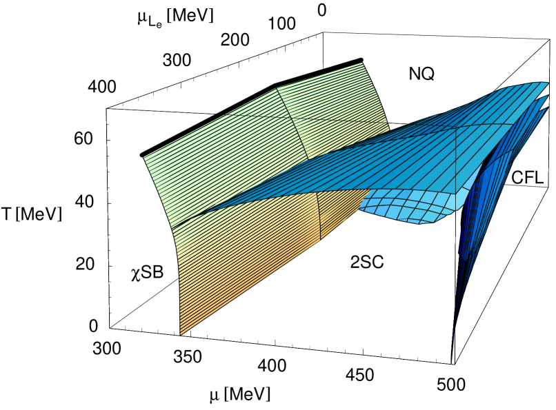
Figure 2.20: The phase diagram of neutral three-flavor quark matter in the three-dimensional space spanned by the quark chemical potential $\mu$, the lepton-number chemical potential $\mu_{L_{e}}$, and the temperature $T$.

In order to discuss the structure of the phase diagram in more details I proceed by showing several two-dimensional slices of it. These are obtained by keeping one of the chemical potentials, $\mu$ or $\mu_{L_{e}}$, fixed and varying the other two parameters.

The $\boldsymbol{T}$–$\boldsymbol{\mu}$ phase diagram

The phase diagrams at two fixed values of the lepton-number chemical potential, $\mu_{L_{e}}=200$ MeV and $\mu_{L_{e}}=400$ MeV are presented in Figs. 2.21 and 2.22. The phase diagram at $\mu_{L_{e}}=0$ MeV, see Fig. 2.12, has already been discussed in Sec. 2.2. The general effects of neutrino trapping can be understood by analyzing the similarities and differences between these three phase diagrams. In this section, I use the same convention for line styles as in Sec. 2.2: thick and thin solid lines denote first-order and second-order phase transitions, respectively; dashed lines indicate the (dis-)appearance of gapless modes in different phases.

Here it is appropriate to note that, in the same model, a schematic version of the $T$–$\mu$ phase diagram at $\mu_{L_{e}}=200$ MeV was first presented in Ref. [133], see the right panel of Fig. 4 there. If one ignores the complications due to the presence of the uSC phase and various gapless phases, the results of Ref. [133] are in qualitative agreement with my findings.

Figure 2.21: The phase diagram of neutral quark matter at a fixed lepton-number chemical potential $\mu_{L_{e}}=200$ MeV.

Figure 2.22: The phase diagram of neutral quark matter at a fixed lepton-number chemical potential $\mu_{L_{e}}=400$ MeV.

In order to understand the basic characteristics of different phases in the phase diagrams in Figs. 2.21 and 2.22, I also present the results for the dynamical quark masses, the gap parameters, and the charge chemical potentials. These are plotted as functions of the quark chemical potential in Figs. 2.23 and 2.24, for two different values of the temperature in the case of $\mu_{L_{e}}=200$ MeV and $\mu_{L_{e}}=400$ MeV, respectively.

Figure 2.23: Dependence of the quark masses, of the gap parameters, and of the electric and color charge chemical potentials on the quark chemical potential at a fixed temperature, $T=0$ MeV (three upper panels) and $T=40$ MeV (three lower panels). The lepton-number chemical potential is kept fixed at $\mu_{L_{e}}=200$ MeV.

In each of the diagrams, there are roughly four distinct regimes. At low temperature and low quark chemical potential, there is a region in which the approximate chiral symmetry is spontaneously broken by large $\bar{\psi}\psi$-condensates. The corresponding phase is denoted by $\chi$SB. In this regime, quarks have relatively large constituent masses which are close to the vacuum values, see Figs. 2.23 and 2.24. Here, the density of all quark flavors is very low and even vanishes at $T=0$. There is no diquark pairing in this phase. The $\chi$SB phase is rather insensitive to the presence of a nonzero lepton-number chemical potential. With increasing $\mu_{L_{e}}$ the phase boundary is only slightly shifted to lower values of $\mu$. This is just another manifestation of the strengthening of the 2SC phase due to neutrino trapping.

With increasing temperature, the $\bar{\psi}\psi$-condensates melt and the $\chi$SB phase turns into the NQ phase where the quark masses are relatively small. Because of the explicit breaking of the chiral symmetry by the current quark masses, there is no need for a phase transition between the two regimes. In fact, at low chemical potentials, I find only a smooth crossover, whereas there is a first-order phase transition in a limited region, 320 MeV $\lesssim\mu\lesssim$ 360 MeV. In contrast to the $\chi$SB regime, the high-temperature NQ phase extends to arbitrary large values of $\mu$. All these qualitative features are little affected by the lepton-number chemical potential.

The third regime is located at relatively low temperatures but at quark chemical potentials higher than in the $\chi$SB phase. In this region, the masses of the up and down quarks have already dropped to values well below their respective chemical potentials while the strange quark mass is still large, see left columns of panels in Figs. 2.23 and 2.24. As a consequence, up and down quarks are quite abundant but strange quarks are essentially absent.

Figure 2.24: Dependence of the quark masses, of the gap parameters, and of the electric and color charge chemical potentials on the quark chemical potential at a fixed temperature, $T=0$ MeV (three upper panels) and $T=40$ MeV (three lower panels). The lepton-number chemical potential is kept fixed at $\mu_{L_{e}}=400$ MeV.

It turns out that the detailed phase structure in this region is very sensitive to the lepton-number chemical potential. At $\mu_{L_{e}}=0$, as discussed in Sec. 2.2, the pairing between up and down quarks is strongly hampered by the constraints of neutrality and $\beta$ equilibrium. As a consequence, there is no pairing at low temperatures, $T\lesssim 10$ MeV, and g2SC-type pairing appears at moderate temperatures, 10 MeV $\lesssim T<T_{c}$ with the value of $T_{c}$ in the range of several dozen MeV, see Fig. 2.12. The situation changes dramatically with increasing the value of the lepton-number chemical potential. Eventually, the low-temperature region of the normal phase of quark matter is replaced by the (g)2SC phase (e.g., at $\mu=400$ MeV, this happens at $\mu_{L_{e}}\simeq 110$ MeV). With $\mu_{L_{e}}$ increasing further, no qualitative changes happen in this part of the phase diagram, except that the area of the (g)2SC phase expands slightly.

Finally, the region in the phase diagram at low temperatures and large quark chemical potentials corresponds to phases in which the cross-flavor strange-nonstrange Cooper pairing becomes possible. In general, as the strength of pairing increases with the quark chemical potential, the system passes through regions of the gapless uSC (guSC), uSC, and gCFL phases and finally reaches the CFL phase. (Of course, the intermediate phases may not always be realized.) The effect of neutrino trapping, which grows with increasing lepton-number chemical potential, is to push out the location of the strange-nonstrange pairing region to larger values of $\mu$. Of course, this is in agreement with the general arguments in Sec. 2.3.2.

Phase	Gapless modes	$\Delta_{1}$	$\Delta_{2}$	$\Delta_{3}$
g2SC	$ru$–$gd$, $gu$–$rd$	$-$	$-$	$\checkmark$
g2SC′	$rd$–$gu$, $gd$–$ru$	$-$	$-$	$\checkmark$
guSC	$rs$–$bu$	$-$	$\checkmark$	$\checkmark$
gCFL	$gs$–$bd$	$\checkmark$	$\checkmark$	$\checkmark$
gCFL′	$rs$–$bu$	$\checkmark$	$\checkmark$	$\checkmark$
gCFL′′	$gs$–$bd$, $rs$–$bu$	$\checkmark$	$\checkmark$	$\checkmark$

Table 2.2: The classification of gapless phases in color-superconducting quark matter. The unmarked gap parameters ($-$) are zero while the checkmarked gap parameters ($\checkmark$) are nonzero in the respective gapless color-superconducting quark phases. The gapless modes $a\alpha$–$b\beta$ are defined by their dispersion relations which interpolate between the dispersion relations of hole-type excitations of $a\alpha$-quarks at small momenta, $k\ll\mu_{\alpha}^{a}$, and particle-type excitations of $b\beta$-quarks at large momenta, $k\gg\mu_{\beta}^{b}$.

Figure 2.25: Dependence of the electron family lepton fraction $Y_{L_{e}}$ for $\mu_{L_{e}}=200$ MeV (thick lines) and $\mu_{L_{e}}=400$ MeV (thin lines) on the quark chemical potential at a fixed temperature, $T=0$ MeV (solid lines), $T=20$ MeV (dashed lines), and $T=40$ MeV (dotted lines).

It is interesting to note that the growth of the strangeness content with increasing quark chemical potential could indirectly be deduced from the behavior of the electric charge chemical potential $\mu_{Q}$ at $T=0$, see the solid lines in the right panels of Figs. 2.23 and 2.24. The value of $\mu_{Q}$ reaches its minimum somewhere in a range of values of the quark chemical potential around $\mu\simeq 440$ MeV. This corresponds to the point where the strange quark chemical potential, $\mu_{s}\simeq\mu-\mu_{Q}/3$, reaches the value of the strange quark mass (see left panels). Hence, there are essentially no strange quarks at lower values of $\mu$, and a rapidly increasing amount of strange quarks at higher values of $\mu$. Since the latter contribute to the electric neutralization, this is a natural explanation for the drop of $|\mu_{Q}|$ above this point.

Figure 2.26: The phase diagram of neutral quark matter in the plane of temperature and lepton-number chemical potential at a fixed value of the quark chemical potential, $\mu=400$ MeV. This phase diagram corresponds to the outer stellar core.

As I mentioned earlier, the presence of the lepton-number chemical potential $\mu_{L_{e}}$ leads to a change of the quark Fermi momenta. This change, in turn, affects Cooper pairing of quarks, facilitating the appearance of some phases and suppressing others. As it turns out, there is also another qualitative effect due to a nonzero value of $\mu_{L_{e}}$. In particular, I find several new variants of gapless phases which do not exist at vanishing $\mu_{L_{e}}$. In Figs. 2.21, 2.22, 2.26, and 2.27, these are denoted by the same names, g2SC or gCFL, but with one or two primes added.

I define the g2SC^′ as the gapless two-flavor color-superconducting phase in which the gapless excitations correspond to $rd$–$gu$ and $gd$–$ru$ modes instead of the usual $ru$–$gd$ and $gu$–$rd$ ones, i.e., $u$ and $d$ flavors are exchanged as compared to the usual g2SC phase. The g2SC^′ phase becomes possible only when the value of $(\mu_{u}^{r}-\mu_{d}^{g})/2\equiv(\mu_{Q}+\mu_{3})/2$ is positive and larger than $\Delta_{3}$. The other phases are defined in a similar manner. In particular, the gCFL^′ phase, which was already introduced in Sec. 2.3.2, is indicated by the gapless $rs$–$bu$ mode, while the gCFL^′′ phase has both, $gs$–$bd$ (as in the gCFL phase) and $rs$–$bu$ gapless modes. The definitions of all gapless phases are summarized in Table 2.2.

The lepton fraction $\boldsymbol{Y_{L_{e}}}$

The numerical results for the lepton fraction $Y_{L_{e}}$ are shown in Fig. 2.25. The thick and thin lines correspond to two different fixed values of the lepton-number chemical potential, $\mu_{L_{e}}=200$ MeV and $\mu_{L_{e}}=400$ MeV, respectively. For a fixed value of $\mu_{L_{e}}$, I find that the lepton fraction changes only slightly with temperature. This is concluded from the comparison of the results at $T=0$ MeV (solid lines), $T=20$ MeV (dashed lines), and $T=40$ MeV (dotted lines) in Fig. 2.25.

Figure 2.27: The phase diagram of neutral quark matter in the plane of temperature and lepton-number chemical potential at a fixed value of the quark chemical potential, $\mu=500$ MeV. This phase diagram corresponds to the inner stellar core. The triangle denotes the transition point from the CFL phase to the gCFL^′ phase at $T=0$.

As is easy to check, at $T=40$ MeV, i.e., when Cooper pairing is not so strong, the $\mu$ dependence of $Y_{L_{e}}$ does not differ very much from the prediction in the simple two-flavor model in Sec. 2.3.2. By saying this, of course, one should not undermine the fact that the lepton fraction in Fig. 2.25 has a visible structure in the dependence on $\mu$ at $T=0$ MeV and $T=20$ MeV. This indicates that quark Cooper pairing plays a nontrivial role in determining the value of $Y_{L_{e}}$.

My numerical study shows that it is hard to achieve values of the lepton fraction more than about $0.05$ in the CFL phase. Gapless versions of the CFL phases, on the other hand, could accommodate the lepton fraction up to about $0.2$ or so, provided the quark and lepton-number chemical potentials are sufficiently large.

From Fig. 2.25, one can also see that the value of the lepton fraction $Y_{L_{e}}\approx 0.4$, i.e., the value expected at the center of the protoneutron star right after its creation, requires a lepton-number chemical potential $\mu_{L_{e}}$ in the range somewhere between $200$ MeV and $400$ MeV, or slightly higher. The larger the quark chemical potential $\mu$, the larger a lepton-number chemical potential $\mu_{L_{e}}$ is needed. Then, in a realistic construction of a protoneutron star, this is likely to result in a noticeable gradient of the lepton-number chemical potential at the initial time. This gradient may play an important role in the subsequent deleptonization due to neutrino diffusion through dense matter.

The $\boldsymbol{T}$–$\boldsymbol{\mu_{L_{e}}}$ phase diagram

Now let me explore the phase diagrams in the plane of temperature and lepton-number chemical potential, keeping the quark chemical potential fixed. Two such slices of the phase diagram are presented in Figs. 2.26 and 2.27. The first one corresponds to a not very large value of the quark chemical potential, $\mu=400$ MeV. This could be loosely termed as the outer stellar core phase diagram. The second one corresponds to $\mu=500$ MeV, and one could associate it with the inner stellar core case. Note, however, that the terms outer stellar core and inner stellar core should not be interpreted literally here. The central densities of (proto-)neutron stars are subject to large theoretical uncertainties and, thus, are not known very well. In the model at hand, the outer stellar core case corresponds to a range of densities around $4n_{0}$, while the inner stellar core case corresponds to a range of densities around $10n_{0}$. These values are of the same order of magnitude that one typically obtains in models (see, e.g., Ref. [48]).

Figure 2.28: Dependence of the quark masses, of the gap parameters, and of the electric and color charge chemical potentials on the temperature at a fixed value of the lepton-number chemical potential, $\mu_{L_{e}}=0$ MeV (three upper panels), $\mu_{L_{e}}=200$ MeV (three middle panels), and $\mu_{L_{e}}=400$ MeV (three lower panels). The quark chemical potential is $\mu=400$ MeV (outer stellar core case).

Figure 2.29: Dependence of the quark masses, of the gap parameters, and of the electric and color charge chemical potentials on the temperature at a fixed value of the lepton-number chemical potential, $\mu_{L_{e}}=0$ MeV (three upper panels), $\mu_{L_{e}}=200$ MeV (three middle panels), and $\mu_{L_{e}}=400$ MeV (three lower panels). The quark chemical potential is $\mu=500$ MeV (inner stellar core case).

In addition to the phase diagrams, I also show the results for the dynamical quark masses, the gap parameters, and the charge chemical potentials. These are plotted as functions of temperature in Fig. 2.28 ($\mu=400$ MeV, outer stellar core case) and in Fig. 2.29 ($\mu=500$ MeV, inner stellar core case), for three different values of the lepton-number chemical potential, $\mu_{L_{e}}=0$ MeV (upper panels), $\mu_{L_{e}}=200$ MeV (middle panels), and $\mu_{L_{e}}=400$ MeV (lower panels).

At first sight, the two phase diagrams in Figs. 2.26 and 2.27 look so different that no obvious connection between them could be made. It is natural to ask, therefore, how such a dramatic change could happen with increasing the value of the quark chemical potential from $\mu=400$ MeV to $\mu=500$ MeV. In order to understand this, it is useful to place the corresponding slices of the phase diagram in the three-dimensional phase diagram in Fig. 2.20.

The $\mu=500$ MeV phase diagram corresponds to the right-hand side surface of the bounding box in Fig. 2.20. This contains almost all complicated phases with strange-nonstrange cross-flavor pairing. The $\mu=400$ MeV phase diagram, on the other hand, is obtained by cutting the three-dimensional phase diagram with a plane parallel to the bounding surface, but going through the middle of the phase diagram. This part of the phase diagram is dominated by the 2SC and NQ phases. Keeping in mind the general structure of the three-dimensional phase diagram, it is also not difficult to understand how the two phase diagrams in Figs. 2.26 and 2.27 transform into each other.

Several comments are in order regarding the zero-temperature phase transition from the CFL to gCFL^′ phase, shown by a small black triangle in the phase diagram at $\mu=500$ MeV, see Fig. 2.27. The appearance of this transition is in agreement with the analytical result in Sec. 2.3.2. Moreover, the critical value of the lepton-number chemical potential also turns out to be very close to the estimate in Eq. (2.188). Indeed, by taking into account that $M_{s}\approx 214$ MeV and $\Delta_{2}\approx 76$ MeV, I obtain $\mu_{L_{e}}^{\mathrm{(cr)}}=\Delta_{2}-M_{s}^{2}/(2\mu)\approx 30$ MeV which agrees well with the numerical value.

In order to estimate how the critical value of $\mu_{L_{e}}$ changes with decreasing the quark chemical potential below $\mu=500$ MeV, one can use the zero-temperature numerical results for $M_{s}$ and $\Delta_{2}$ from Sec. 2.2. Then, one arrives at the following power-law fit for the $\mu$-dependence of the critical value:

$$\mu_{L_{e}}^{\mathrm{(cr)}}\approx 0.00575\leavevmode\nobreak\ \mathrm{MeV}^{-1}\left(\mu-457.4\leavevmode\nobreak\ \mathrm{MeV}\right)\left(622.1\leavevmode\nobreak\ \mathrm{MeV}-\mu\right)\;,$$ (2.190)

for 457.4 MeV $\leq\mu\leq$ 500 MeV. Note that the CFL phase does not appear at $T=0$ when $\mu<457.4$ MeV, cf. Fig. 2.12. With increasing the values of the quark chemical potential above $\mu=500$ MeV, one expects that the critical value of $\mu_{L_{e}}$ should continue to increase for a while, and then decrease when the effects of the cutoff start to suppress the size of the gap $\Delta_{2}$. However, the validity of the fit in Eq. (2.190) is questionable there because no numerical data for $\mu>500$ MeV was used in its derivation.

A schematic version of the phase diagram in the $T$–$\mu_{L_{e}}$ plane was presented earlier in Ref. [133], see the left panel in Fig. 4 there. In Ref. [133], the value of the quark chemical potential was $\mu=460$ MeV, and therefore a direct comparison with my results is not easy. One can see, however, that the diagram of Ref. [133] fits naturally into the three-dimensional diagram in Fig. 2.20. Also, the diagram of Ref. [133] is topologically close to my version of the phase diagram at $\mu=500$ MeV which is shown in Fig. 2.27. The quantitative difference is not surprising: the region of the (g)CFL phase is considerably larger at $\mu=500$ MeV than at $\mu=460$ MeV.

Chapter 3 Conclusions

The phase diagram of neutral quark matter was poorly understood as I began with the research on this topic in 2003, see Fig. 1.1. The task of my thesis is to illuminate the phase structure of neutral quark matter. From the phase diagram of neutral quark matter, one can predict in which state is neutral quark matter in the cores of neutron stars which are most probably the candidates for neutral color-superconducting quark matter in nature.

3.1 Summary and discussion

In Chapter 1, I gave an introduction to quark matter, color superconductivity, and stellar evolution. I presented the most important color-superconducting quark phases and explained how stars evolve and become neutron stars. At extremely large densities which are probably present in the cores of neutron stars, there is a dominant attractive interaction between the quarks that causes the formation of quark Cooper pairs [10, 11, 12]. This causes color superconductivity. Since quarks are spin-$\frac{1}{2}$ fermions which appear in various colors and flavors, there are many possibilities of forming quark Cooper pairs. This is why there exist many different color-superconducting quark phases.

In order to predict which of these phases are energetically preferred in nature, it is necessary to compute the phase diagram of neutral quark matter and to determine which phases are dominant at a given temperature and quark chemical potential. The phase diagram of neutral quark matter consisting of up, down, and strange quarks is presented in Chapter 2. In this context, it is important to consider neutral quark matter because otherwise there would occur repulsive Coulomb forces which lead to the explosion of the neutron stars. Quark matter has to be color neutral because color-charged objects have never been seen in nature. Besides, color-charged neutron stars would be unstable. Matter inside neutron stars is in $\beta$ equilibrium which means that neutron-star matter is in equilibrium with respect to weak interactions.

In Sec. 2.1, I studied massless neutral three-flavor quark matter at large baryon densities within an NJL model. The effects of the strange quark mass were incorporated by a shift of the chemical potential of strange quarks, see Eq. (2.35). This shift reflects the reduction of the Fermi momenta of strange quarks due to their mass. Such an approach is certainly reliable at small values of the strange quark mass. In Ref. [113], where the strange quark mass was properly taken into account, I confirmed that it is also qualitatively correct at large values of the strange quark mass. I obtained a very rich phase structure by varying the strange quark mass, the quark chemical potential, and the temperature.

At $T=0$, there are two main possibilities for the strange quark matter ground state: the CFL and gCFL phases. These findings confirm the results of Refs. [90, 91] concerning the existence of the gCFL phase, the estimate of the critical value of the strange quark mass $m_{s}$, and the dependence of the chemical potentials on $m_{s}$. I also confirmed that it is the color-neutrality condition, controlled by the color chemical potential $\mu_{8}$ which drives the transition from the CFL to the gCFL phase [90, 91]. This is in contrast to gapless two-flavor color superconductivity which results from electrical neutrality [84, 85].

Because I use a nine-parameter ansatz for the gap matrix, see Eq. (2.53), the results of Sec. 2.1 are more general than those of Refs. [90, 91]. For example, I was able to explicitly study the effects of the symmetric pairing channel, described by the sextet gap parameters, that were neglected in Refs. [90, 91]. As one might have expected, these latter modify the quasiparticle dispersion relations only slightly. This check was important, however, to see that the zero-temperature phase transition from the CFL phase to the gCFL phase, which is not associated with any symmetry, is robust against such a deformation of the quark system.

In Sec. 2.1, I also studied the temperature dependence of the gap parameters and the quasiparticle spectra. In particular, this study revealed that there exist several different phases of neutral three-flavor quark matter that have been predicted in the framework of the Ginzburg-Landau-type effective theory in Ref. [111]. My results extend the near-critical behavior discussed in Ref. [111] to all temperatures. Also, I show how this behavior evolves with changing the value of the strange quark mass. The only real qualitative difference between my results and the results of Refs. [111, 112] is that, instead of the dSC phase, I find the uSC phase in the phase diagram. In Ref. [113], I confirmed the results of Sec. 2.1 regarding the existence of several different phases of neutral three-flavour quark matter at nonzero temperature. I also confirmed the order in which they appear. In particular, I observed the appearance of the uSC phase as an intermediate state in the melting of the (g)CFL phase into the 2SC phase. Formally, this is different from the prediction of Ref. [111]. I find, however, that the difference is connected with the choice of the model parameters. In the NJL model with a cutoff parameter of 800 MeV used in Ref. [112], there is a non-vanishing (although rather small) region of the dSC phase. On the other hand, in the NJL model with a relatively small cutoff parameter of 653.3 MeV, no sizeable window of the dSC phase can be found. Therefore, I conclude that the appearence of the uSC or dSC phase, repectively, is very sensitive to the choice of the model parameters, or more precisely, it depends strongly on the cutoff parameter.

The main result of Sec. 2.1 is the complete phase diagram of massless neutral three-flavor quark matter in the $T$–$m_{s}^{2}/\mu$ and $T$–$\mu$ plane, shown in Fig. 2.11. In this figure, all symmetry-related phase transitions are denoted by solid lines. (The symmetries of all phases appearing in this figure were discussed in Ref. [111].) The dashed lines in Fig. 2.11 separate the mCFL and regular 2SC phases from the gCFL and g2SC phases. These cannot be real phase transitions, but are at most smooth crossovers. At $T=0$, there is an insulator-metal phase transition between the CFL and the gCFL phase [90, 91]. At nonzero temperature, there exists a similar insulator-metal-type transition between the CFL and the mCFL phase, given by the dotted lines in Fig. 2.11.

In Sec. 2.2, I studied the $T$–$\mu$ phase diagram of neutral three-flavor quark matter within the NJL model of Ref. [136] in which chiral symmetry is broken explicitly by small but nonzero current quark masses. As in the previous study in Sec. 2.1, I used the mean-field approximation in the analysis. In contrast to Sec. 2.1, in Sec. 2.2, the constituent quark masses were treated self-consistently as dynamically generated quantities. The main results were summarized in Figs. 2.12 and 2.13.

By comparing the phase diagram of massless quarks shown in the right panel of Fig. 2.11 with the phase diagram shown in Fig. 2.12, I noticed several important differences. First of all, I observed that a self-consistent treatment of quark masses strongly influences the competition between different quark phases. As was noticed earlier in Ref. [139], there exists a subtle interplay between the two main effects. On the one hand, the actual values of the quark masses directly influence the competition between different normal and color-superconducting phases. On the other hand, competing phases themselves determine the magnitude of the masses. Very often, this leads to first-order phase transitions in which certain regions in the mass-parameter space become inaccessible.

Some differences to the results in Sec. 2.1 and Sec. 2.2 are related to a different choice of model parameters. Most importantly, the value of the diquark coupling $G_{D}=\frac{3}{4}G_{S}$ is considerably weaker in the NJL model of Sec. 2.2. This can be easily seen by comparing the magnitude of the zero-temperature gap at a given value of the quark chemical potential, say at $\mu=500$ MeV, in the two models. It is $\Delta_{0}^{\mathrm{(500)}}\approx 140$ MeV in Sec. 2.1 and $\Delta_{0}^{\mathrm{(500)}}\approx 76$ MeV in Sec. 2.2. (Note that the strength of the diquark pairing in Ref. [112] is even weaker, corresponding to $\Delta_{0}^{\mathrm{(500)}}\approx 20$ MeV.) It should be noted that even the strong coupling $G_{D}=G_{S}$ which leads to $\Delta_{0}^{\mathrm{(500)}}\approx 120$ MeV, is still slightly weaker than that in Sec. 2.1. In this case, however, the corresponding results differ mostly because the quark masses are treated very differently.

Because of the weaker diquark coupling strength, the Cooper instabilities in Fig. 2.12 occur systematically at higher values of the quark chemical potential than in the right panel of Fig. 2.11. In particular, this is most clearly seen from the critical lines of the transition to the (g)CFL phase. Another consequence of the weaker interaction is the possibility of a thermal enhancement of the (g)2SC Cooper pairing at intermediate values of the quark chemical potential. This kind of enhancement was studied in detail in Refs. [84, 85]. Making use of the same arguments, one can tell immediately how the phase diagram in Fig. 2.12 should change with increasing or decreasing the diquark coupling strength.

In particular, with increasing (decreasing) the diquark coupling strength, the region of the (g)2SC phase at intermediate values of the quark chemical potential should expand (shrink) along the temperature direction. The regions covered by the other (i.e., uSC and CFL) phases should have qualitatively the same shape, but shift to lower (higher) values of the quark chemical potential and to higher (lower) values of the temperature. In the case of strong coupling, in particular, these general arguments are confirmed by my numerical calculations. The corresponding phase diagram is shown in Fig. 2.13.

Several comments are in order regarding the choice of the NJL model used in Sec. 2.2. The model is defined by the set of parameters in Eq. (2.119) which were fitted to reproduce several important QCD properties in vacuum [136]. (Note that the same model also was used in Ref. [133].) It is expected, therefore, that this is a reasonable effective model of QCD that captures the main features of both, chiral and color-superconducting pairing dynamics. Also, a relatively small value of the cutoff parameter in the model, see Eq. (2.119), should not necessarily be viewed as a bad feature of the model. In fact, this might simply mimic a natural property of the full theory in which the coupling strength of relevant interactions is quenched at large momenta.

In this relation, note that the approach of Ref. [112] regarding the cutoff parameter in the NJL model is very different. It is said there that a large value of this parameter is beneficial in order to extract results which are insensitive to a specific choice of the cutoff. However, I do not find any physical argument that would support this requirement. Instead, I insist on having an effective model that describes reasonably well the QCD properties at zero quark chemical potential. I do not pretend, of course, that a naïve extrapolation of the model to large densities can be rigorously justified. In absence of a better alternative, however, this seems to be the only sensible choice.

The results of Sec. 2.2 might be relevant for understanding the physics of (hybrid) neutron stars with quark cores, in which the deleptonization is completed. In order to obtain a phase diagram that could be applied to protoneutron stars, one has to generalize the analysis to take into account neutrino trapping.

In Sec. 2.3, I studied the effect of neutrino trapping on the phase diagram of neutral three-flavor quark matter within the NJL model of Ref. [136]. The results were obtained in the mean-field approximation, treating constituent quark masses as dynamically generated quantities. The overall structure of the phase diagram in the space of three parameters, namely temperature $T$, quark chemical potential $\mu$ and lepton-number chemical potential $\mu_{L_{e}}$, was summarized in Fig. 2.20. This was further detailed in several two-dimensional slices of the phase diagram, including phase diagrams in the plane of temperature and quark chemical potential (see Figs. 2.21 and 2.22) and in the plane of temperature and lepton-number chemical potential (see Figs. 2.26 and 2.27).

By making use of simple model-independent arguments, as well as detailed numerical calculations in the framework of the NJL model, I found that neutrino trapping helps Cooper pairing in the 2SC phase and suppresses the CFL phase. In essence, this is the consequence of satisfying the electric neutrality constraint in the quark system. In two-flavor quark matter, the (positive) lepton-number chemical potential $\mu_{L_{e}}$ helps to provide extra electrons without inducing a large mismatch between the Fermi momenta of up and down quarks. With reducing the mismatch, of course, Cooper pairing gets stronger. This is in sharp contrast to the situation in the CFL phase of quark matter, which is neutral in the absence of electrons. Additional electrons due to large $\mu_{L_{e}}$ can only put extra stress on the system.

In application to protoneutron stars, my findings in Sec. 2.3 strongly suggests that the CFL phase is very unlikely to appear during the early stage of the stellar evolution before the deleptonization is completed. If color superconductivity occurs there, the 2SC phase is the best candidate for the ground state. In view of this finding, it might be quite natural to suggest that matter inside protoneutron stars contains little or no strangeness (just as the cores of the progenitor stars) during the early times of their evolution. In this connection, it is appropriate to recall that neutrino trapping also suppresses the appearance of strangeness in the form of hyperonic matter and kaon condensation [48]. My finding, therefore, is a special case of a generic property.

The authors of Ref. [83] claimed that the 2SC phase is absent in compact stars and underpinned their claim by using a very simple model-independent calculation. The phase diagrams which were created by using more precise NJL-type models and which are shown in my thesis are the best evidence that there indeed could exist a 2SC phase in compact stars and that the 2SC phase in general is not absent. This is always the case in protoneutron stars and in cold neutron stars at large diquark coupling constants. But in the limit of weak diquark coupling and zero temperature in which the simple model-independent calculation in Ref. [83] is valid, the statement seems to be true that the 2SC phase is absent, cf. Fig. 2.12.

After the deleptonization occurs, it is possible that the ground state of matter at high density in the central region of neutron stars is the CFL phase. This phase contains a large number of strange quarks. Therefore, an abundant production of strangeness should happen right after the deleptonization in protoneutron stars. If realized in nature, in principle this scenario may have observational signatures.

3.2 Open questions and outlook

The quark sector of the phase diagram of strongly interacting matter was poorly understood in 2003, see Fig. 1.1. With my investigations of this subject, I made the first attempt to illuminate the phase structure in the quark sector of the phase diagram of strongly interacting matter within the framework of an NJL model. In Fig. 3.1, I finally show the status of knowledge about the phase diagram of strongly interacting matter in 2005.

With my investigations I took the first step in order to study the phase diagram of neutral quark matter, see Ref. [110] and Sec. 2.1. I further improved my result for the phase diagram of neutral quark matter by properly incorporating the strange quark mass [113]. The next step in my investigation was to treat the quark masses self-consistently as dynamically generated quantities, see Ref. [114] and Sec. 2.2, and finally to incorporate a nonzero lepton-number chemical potential, see Ref. [116] and Sec. 2.3.

Here, I restricted my study to spin-zero color-superconducting phases only which seem to be the most preferred color-superconducting states because they have the highest pressure. Therefore, I do not expect that other than these color-superconducting states which I have investigated in this thesis will occur in the phase diagram of neutral quark matter. But if the pressures of one or more of these other color-superconducting quark phases are larger than those of the spin-zero color-superconducting quark phases so that these other color-superconducting quark phases indeed will occur in the phase diagram of neutral quark matter, then I expect that the regions of such color-superconducting phases in the phase diagram are small so that the phase diagram in Fig. 2.12 will not be changed very much. In order to avoid misunderstandings, I want to say that I do not expect that such color-superconducting states occur in the phase diagram of neutral quark matter. I do not say that such color-superconducting phases are absent.

An example for a possible occurrence of a color-superconducting phase which I have not considered in my investigations is the spin-one color-superconducting transverse CSL phase (the most preferred spin-one color-superconducting quark phase [39]). This phase has good chances to occur very close to the axis of the quark chemical potential in the region of the normal quark phase in the phase diagram of neutral quark matter in Fig. 2.12. If one will find that this is really true then the phase diagram of neutral quark matter shown in Fig. 2.12 will not be changed much because spin-one color-superconducting quark phases like the transverse CSL phase will be destroyed even at small temperatures. Therefore, the line width of the axis of the quark chemical potential is possibly thicker than the region of the spin-one color-superconducting transverse CSL phase in the phase diagram of neutral quark matter. Nevertheless, the CSL phase could occur in cold neutron stars [38].

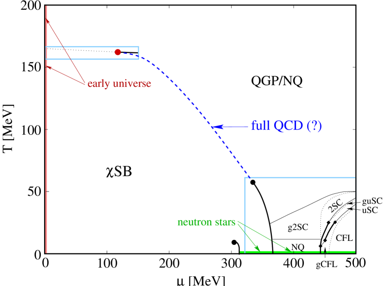
Figure 3.1: The knowledge about the phase diagram of strongly interacting matter in 2005. The upper left part shows the critical endpoint of the quark-hadron phase transition which is obtained by lattice QCD calculations [5]. The lower right part shows the phase diagram of neutral three-flavor quark matter [114], where quark masses are treated self-consistently, see Fig. 2.12. The dashed line shows the discrepancy between the critical endpoint of the quark-hadron phase transition in the NJL model with that obtained in lattice QCD calculations. This discrepancy could be resolved by using full QCD. In addition, there is shown the state of the early universe and of cold neutron stars after deleptonization.

In Ref. [143], another possible spin-zero color-superconducting quark phase, the A-phase, was checked if it occurs in the phase diagram of neutral quark matter. The result was that this phase always has a lower pressure than the phases which I have investigated in my thesis. Therefore, the A-phase does not appear in the phase diagram of neutral quark matter.

However, it will be very important to check if other than these color-superconducting phases which I have investigated in this thesis indeed occur in the phase diagram of neutral quark matter (see Ref. [144], where some of these other color-superconducting quark phases are shown). Such an investigation is outside the scope of my thesis. Much work concerning this check has to be done in future. The pressures of all competing phases have to be compared. The phase with the highest value of the pressure is the preferred one and therefore appears in the phase diagram of neutral quark matter.

Despite the progress in understanding the phase diagram of neutral quark matter, there still exists a fundamental problem. Gapless color-superconducting quark phases are unstable in some regions of the phase diagram of neutral quark matter because of chromomagnetic instabilities [92] so that another phase will be the preferred state. Chromomagnetic instabilities occur even in regular color-superconducting quark phases. The author of Ref. [93] shows that chromomagnetic instabilities occur only at low temperatures in neutral color-superconducting quark matter. The author of Ref. [94] points out that the instabilities might be caused by using BCS theory in mean-field approximation, where phase fluctuations have been neglected. With the increase of the mismatch between the Fermi surfaces of paired fermions, phase fluctuations play more and more an important role, and soften the superconductor. Strong phase fluctuations will eventually quantum-disorder the superconducting state, and turn the system into a phase-decoherent pseudogap state. By using an effective theory of the CFL state, the author of Ref. [95] demonstrates that the chromomagnetic instability is resolved by the formation of an inhomogeneous meson condensate. The authors of Ref. [96] describe a new phase in neutral two-flavor quark matter within the framework of the Ginzburg-Landau approach, in which gluonic degrees of freedom play a crucial role. They call it a gluonic phase. In this phase, gluon condensates cure a chromomagnetic instability in the 2SC solution and lead to spontaneous breakdown of the color gauge symmetry, the $[U(1)_{\mathrm{em}}]$ and the rotational $SO(3)$ group. In other words, the gluonic phase describes an anisotropic medium in which color and electric superconductivity coexist. In Ref. [97], it was suggested that the chromomagnetic instability in gapless color-superconducting phases indicates the formation of the LOFF phase [98] which is discussed in Ref. [99] in the context of quark matter. Other possibilities could be the formation of a spin-one color-superconducting quark phase, a mixed phase, or a completely new state. The authors of Ref. [100] suggest that a mixed phase composed of the 2SC phase and the normal quark phase may be more favored if the surface tension is sufficiently small [101]. The authors of Ref. [102] suggest a single first-order phase transition between CFL and nuclear matter. Such a transition, in space, could take place either through a mixed phase region or at a single sharp interface with electron-free CFL and electron-rich nuclear matter in stable contact. The authors of Ref. [102] constructed a model for such an interface.

Another possibility in order to avoid gapless color-superconducting quark phases is to set the diquark coupling constant to such high values that gapless phases will not occur in the phase diagram [118]. But then it is another question if such large diquark coupling constants indeed occur in nature. My personal opinion is that one should not increase the diquark coupling constant to such high values in order to get rid of the problem but use the standard value of the diquark coupling constant in Eq. (2.120) which is predicted by the Fierz transformation in vacuum.

Whether gapless phases can indeed exist as color-superconducting quark phases or whether they will be unstable because of chromomagnetic instabilities is not known yet. Also, if they are unstable, it is not yet known which states will be formed in the respective regions of the phase diagram. Such an investigation is outside the scope of my thesis, and much work has to be done in future to solve this problem. The pressures of all competing quark phases have to be determined in these regions of the phase diagram. The phase with the highest value of the pressure is the preferred one.

Another problem which has to be solved is the discrepancy between the critical endpoint of the quark-hadron phase transition which is obtained by lattice QCD calculations [5] and NJL models [106, 114, 115, 116, 118, 138, 139], see also Fig. 3.1. It is appropriate to mention here that the location of the critical endpoint might be affected very much by fluctuations of the composite chiral fields. These are not included in the mean-field studies of the NJL model. In fact, this is probably the main reason for their inability to pin down the location of the critical endpoint consistent for example, with lattice QCD calculations [5]. It is fair to mention that the current lattice QCD calculations are not very reliable at nonzero $\mu$ either. Therefore, the predictions of my thesis, as well as of those in Refs. [106, 114, 115, 116, 118, 138, 139], regarding the critical endpoint cannot be considered as very reliable. One definitely will be able to say where exactly the critical endpoint is located and how the phase diagram of neutral quark matter looks like if one uses full QCD. Such an investigation is outside the scope of my thesis and has to be done in future. Since the NJL-type models used in my thesis fulfill at least some important key features of QCD, I expect that the phase diagram of neutral quark matter which is shown in Fig. 2.12 will be changed only quantitatively so that the overall phase structure does not change if one computes a more realistic phase diagram of neutral quark matter by using full QCD.

In the context of compact stars, it is not known yet if their cores reach chemical potentials which make color superconductivity possible. It is of great importance to resolve this issue. Neutron stars are the most likely candidates for color superconductivity in nature and therefore, one expects that they contain color-superconducting quark cores. Therefore, one has to find an experimental proof for color-superconducting quark matter. This can be done by detecting neutrino and $\gamma$-emissions of protoneutron stars and in colliders.

Since one does not know yet how large the lepton-number chemical potential in protoneutron stars is during their evolution from the supernova explosion until they become a cold neutron star, it is difficult to say exactly, through which phases they go in the three-dimensional phase diagram shown in Fig. 2.20. Therefore, it would be very interesting to study the precise evolution path of protoneutron stars in the three-dimensional phase diagram.

I note that the analysis in this thesis is restricted to locally neutral phases only. This automatically excludes, for example, crystalline [99] and mixed [101, 100, 120] phases. Also, in the mean field approximation utilized here, I cannot get any phases with meson condensates [28, 29, 30].

In nature, phase transitions can take place either through sharp boundaries between pure phases which are located next to each other or through mixed-phase regions. In this thesis, I considered only the former possibility, where each phase has the highest pressure in its region of the phase diagram and where the pressures of the phases are equal only at the sharp phase boundaries. Such phase transitions are obtained by so-called Maxwell constructions. It would be interesting to study the possibility of mixed phases by making so-called Gibbs constructions [145], in which the pressures and the chemical potentials of the phases are equal and continuous in contrast to Maxwell constructions.

Another interesting investigation in the context of compact stars would be to create a phase-radius diagram that shows which phase occurs at which radius of the compact star. Such a diagram would directly show the composition and structure of a compact star.

Appendix A Definitions of matrices

In this chapter of the Appendix, I present some definitions such as the Pauli and $\gamma$-matrices, and the generatores of the $SU(3)$ group. I also show the chirality, energy, energy-chirality, and the spin projectors as well as their properties.

A.1 The Pauli matrices

The Pauli matrices are defined as:

$$\sigma_{1} =\left(\begin{array}[]{r@{\hspace{4mm}}r}0\hskip 11.38109pt&1\\ 1\hskip 11.38109pt&0\end{array}\right)\;, \sigma_{2} =\left(\begin{array}[]{rr}0&-i\\ i&0\end{array}\right)\;,$$ (A.1)

$$\sigma_{3} =\left(\begin{array}[]{rr}1&0\\ 0&-1\end{array}\right)\;, \boldsymbol{\sigma} =\left(\sigma_{1},\sigma_{2},\sigma_{3}\right)\;.$$

The Pauli matrices are hermitian,

$$\sigma_{i}^{\dagger}=\sigma_{i}\;.$$ (A.2)

The following relations are valid:

$$\sigma_{i}^{2}=1\;,\qquad\sigma_{i}\sigma_{j}=i\sigma_{k}\;,\qquad\left[\sigma_{i},\sigma_{j}\right]=2i\sigma_{k}\;,\qquad\left\{\sigma_{i},\sigma_{j}\right\}=2\delta_{ij}\;.$$ (A.3)

A.1.1 Spin projectors

The spin projectors are defined as

$$\mathcal{P}_{s}\left(\mathbf{k}\right)=\frac{1}{2}\,(1+s\boldsymbol{\sigma}\cdot\hat{\mathbf{k}})\;,$$ (A.4)

where $s=\pm$ corresponds to the projections onto spin up or spin down states, respectively, and $\boldsymbol{\sigma}$ are the Pauli matrices. The spin projectors fulfill the properties of completeness and orthogonality,

$$\mathcal{P}_{+}\left(\mathbf{k}\right)+\mathcal{P}_{-}\left(\mathbf{k}\right) = 1\;,$$ (A.5a)

$$\mathcal{P}_{s}\left(\mathbf{k}\right)\mathcal{P}_{s^{\prime}}\left(\mathbf{k}\right) = \delta_{ss^{\prime}}\mathcal{P}_{s^{\prime}}\left(\mathbf{k}\right)\;.$$ (A.5b)

The spin projectors are hermitian,

$$\mathcal{P}_{s}^{\dagger}\left(\mathbf{k}\right)=\mathcal{P}_{s}\left(\mathbf{k}\right)\;.$$ (A.6)

The following relations are valid:

$$\mathcal{P}_{+}\left(\mathbf{k}\right)-\mathcal{P}_{-}\left(\mathbf{k}\right) = \boldsymbol{\sigma}\cdot\hat{\mathbf{k}}\;,$$ (A.7)

$$\mathrm{Tr}\,\mathcal{P}_{s}\left(\mathbf{k}\right) = 1\;.$$ (A.8)

A.2 Matrices in Dirac space

The Dirac definition of the $\gamma$-matrices reads:

$$\gamma^{0} =\left(\begin{array}[]{r@{\hspace{2mm}}r}1\hskip 5.69054pt&0\\ 0\hskip 5.69054pt&-1\end{array}\right)\;, \gamma^{1} =\left(\begin{array}[]{c@{\hspace{2mm}}l}\ 0\hfil\hskip 5.69054pt&\sigma_{1}\\ -\sigma_{1}\hfil\hskip 5.69054pt&0\end{array}\right)\;,$$ (A.9)

$$\gamma^{2} =\left(\begin{array}[]{c@{\hspace{2mm}}l}\ 0\hfil\hskip 5.69054pt&\sigma_{2}\\ -\sigma_{2}\hfil\hskip 5.69054pt&0\end{array}\right)\;, \gamma^{3} =\left(\begin{array}[]{c@{\hspace{2mm}}l}\ 0\hfil\hskip 5.69054pt&\sigma_{3}\\ -\sigma_{3}\hfil\hskip 5.69054pt&0\end{array}\right)\;,$$

$$\boldsymbol{\gamma} =\left(\begin{array}[]{c@{\hspace{3mm}}l}\ \ 0\hfil\hskip 8.53581pt&\boldsymbol{\sigma}\\ -\boldsymbol{\sigma}\hfil\hskip 8.53581pt&0\end{array}\right)\;, \gamma_{5} =\left(\begin{array}[]{r@{\hspace{3mm}}r}0\hskip 8.53581pt&1\\ 1\hskip 8.53581pt&0\end{array}\right)=i\gamma^{0}\gamma^{1}\gamma^{2}\gamma^{3}\;.$$

The following relations are valid:

$$\begin{gathered}\gamma_{0}^{2}=1\;,\qquad\left(\gamma^{i}\right)^{2}=-1\;,\qquad\gamma_{5}^{2}=1\;,\\ \gamma^{\mu}=\left(\gamma^{0},\gamma^{1},\gamma^{2},\gamma^{3}\right)=\left(\gamma^{0},\boldsymbol{\gamma}\right)\;,\qquad\gamma_{0}\left(\gamma^{\mu}\right)^{\dagger}\gamma_{0}=\gamma^{\mu}\;,\qquad\left\{\gamma^{\mu},\gamma^{\nu}\right\}=2g^{\mu\nu}\;,\end{gathered}$$ (A.10)

where

$$g^{\mu\nu}=\mathrm{diag}\left(1,-1,-1,-1\right)$$ (A.11)

is the metric tensor. The charge-conjugation matrix in Dirac representation is defined as

$$C=i\gamma^{2}\gamma_{0}\;,$$ (A.12)

where $\gamma^{2}$ is given by Eq. (A.9). The following relations are valid:

$$C=-C^{-1} = -C^{T}=-C^{\dagger}\;,$$ (A.13a)

$$C\gamma^{\mu}C^{-1} = -\left(\gamma^{\mu}\right)^{T}\;,$$ (A.13b)

$$C\left(\gamma^{\mu}\right)^{T}C^{-1} = -\gamma^{\mu}\;.$$ (A.13c)

With the charge-conjugation matrix, one can introduce the charge-conjugate spinors in space-time,

$$\psi_{C}\left(X\right) =C\bar{\psi}^{T}\left(X\right)\;,$$ (A.14)

$$\bar{\psi}_{C}\left(X\right) =\psi^{T}\left(X\right)C\;,$$

$$\psi\left(X\right) =C\bar{\psi}_{C}^{T}\left(X\right)\;,$$

$$\bar{\psi}\left(X\right) =\psi_{C}^{T}\left(X\right)C\;,$$

and in energy-momentum space,

$$\psi_{C}\left(K\right) =C\bar{\psi}^{T}\left(-K\right)\;,$$ (A.15)

$$\bar{\psi}_{C}\left(K\right) =\psi^{T}\left(-K\right)C\;,$$

$$\psi\left(-K\right) =C\bar{\psi}_{C}^{T}\left(K\right)\;,$$

$$\bar{\psi}\left(-K\right) =\psi_{C}^{T}\left(K\right)C\;.$$

A.2.1 Projectors in Dirac space

In the limit of vanishing mass, the chirality, energy, and energy-chirality projectors are defined as:

$$\mathcal{P}_{c} = \textstyle\frac{1}{2}\displaystyle\,(1+c\gamma_{5})\;,$$ (A.16a)

$$\Lambda^{e}\left(\mathbf{k}\right) = \textstyle\frac{1}{2}\displaystyle\,(1+e\gamma_{0}\boldsymbol{\gamma}\cdot\hat{\mathbf{k}})\;,$$ (A.16b)

$$\mathcal{P}_{c}^{e}\left(\mathbf{k}\right) \equiv \mathcal{P}_{c}\,\Lambda^{e}\left(\mathbf{k}\right)=\textstyle\frac{1}{4}\displaystyle\,(1+c\gamma_{5})\,(1+e\gamma_{0}\boldsymbol{\gamma}\cdot\hat{\mathbf{k}})\;,$$ (A.16c)

where $c=\pm$ or $c=r,\ell$, respectively, stands for right-handed and left-handed projections, and $e=\pm$ for projections onto states of positive and negative energy. The chirality and energy projectors fulfill the properties of completeness and orthogonality,

$$\mathcal{P}_{r}+\mathcal{P}_{\ell} = 1\;,$$ (A.17a)

$$\Lambda^{+}\left(\mathbf{k}\right)+\Lambda^{-}\left(\mathbf{k}\right) = 1\;,$$ (A.17b)

$$\mathcal{P}_{c}\mathcal{P}_{c^{\prime}} = \delta_{c,c^{\prime}}\mathcal{P}_{c^{\prime}}\;,$$ (A.17c)

$$\Lambda^{e}\left(\mathbf{k}\right)\Lambda^{e^{\prime}}(\mathbf{k}) = \delta^{e,e^{\prime}}\Lambda^{e^{\prime}}(\mathbf{k})\;.$$ (A.17d)

These projectors are hermitian,

$$\mathcal{P}_{c}^{\dagger} = \mathcal{P}_{c}\;,$$ (A.18a)

$$\left[\Lambda^{e}\right]^{\dagger}\left(\mathbf{k}\right) = \Lambda^{e}\left(\mathbf{k}\right)\;,$$ (A.18b)

and they commute with each other,

$$\left[\mathcal{P}_{c},\Lambda^{e}\left(\mathbf{k}\right)\right]=0\;.$$ (A.19)

The energy-chirality projectors fulfill the properties of completeness and orthogonality,

$$\sum_{c,e}\mathcal{P}_{c}^{e}\left(\mathbf{k}\right) = 1\;,$$ (A.20a)

$$\mathcal{P}_{c}^{e}\left(\mathbf{k}\right)\mathcal{P}_{c^{\prime}}^{e^{\prime}}\left(\mathbf{k}\right) = \delta_{c,c^{\prime}}\delta^{e,e^{\prime}}\mathcal{P}_{c^{\prime}}^{e^{\prime}}\left(\mathbf{k}\right)\;.$$ (A.20b)

The energy-chirality projectors are hermitian,

$$\left[\mathcal{P}_{c}^{e}\right]^{\dagger}\left(\mathbf{k}\right)=\mathcal{P}_{c}^{e}\left(\mathbf{k}\right)\;.$$ (A.21)

The following relations are valid:

$$\mathcal{P}_{-c}^{-e}\left(\mathbf{k}\right) = \gamma_{0}\mathcal{P}_{c}^{e}\left(\mathbf{k}\right)\gamma_{0}\;,$$ (A.22)

$$\Lambda^{+}\left(\mathbf{k}\right)-\Lambda^{-}\left(\mathbf{k}\right) = \gamma_{0}\boldsymbol{\gamma}\cdot\hat{\mathbf{k}}\;,$$ (A.23)

$$\mathrm{Tr}\,\mathcal{P}_{c}^{e}\left(\mathbf{k}\right) = 1\;,$$ (A.24)

$$\mathcal{P}_{c}\gamma^{\mu} = \gamma^{\mu}\mathcal{P}_{-c}\;.$$ (A.25)

A.3 The generators of the SU(3) group

The generators of the $SU(3)$ group are defined as:

$$T_{1} =\frac{1}{2}\left(\begin{array}[]{r@{\hspace{4mm}}r@{\hspace{4mm}}r}0\hskip 11.38109pt&1\hskip 11.38109pt&0\\ 1\hskip 11.38109pt&0\hskip 11.38109pt&0\\ 0\hskip 11.38109pt&0\hskip 11.38109pt&0\end{array}\right)\;, T_{2} =\frac{1}{2}\left(\begin{array}[]{rr@{\hspace{4mm}}r}0&-i\hskip 11.38109pt&0\\ i&0\hskip 11.38109pt&0\\ 0&0\hskip 11.38109pt&0\end{array}\right)\;,$$ (A.26)

$$T_{3} =\frac{1}{2}\left(\begin{array}[]{rr@{\hspace{4mm}}r}1&0\hskip 11.38109pt&0\\ 0&-1\hskip 11.38109pt&0\\ 0&0\hskip 11.38109pt&0\end{array}\right)\;, T_{4} =\frac{1}{2}\left(\begin{array}[]{r@{\hspace{3mm}}r@{\hspace{3mm}}r}0\hskip 8.53581pt&0\hskip 8.53581pt&1\\ 0\hskip 8.53581pt&0\hskip 8.53581pt&0\\ 1\hskip 8.53581pt&0\hskip 8.53581pt&0\end{array}\right)\;,$$

$$T_{5} =\frac{1}{2}\left(\begin{array}[]{r@{\hspace{3mm}}rr}0\hskip 8.53581pt&0&-i\\ 0\hskip 8.53581pt&0&0\\ i\hskip 8.53581pt&0&0\end{array}\right)\;, T_{6} =\frac{1}{2}\left(\begin{array}[]{r@{\hspace{3mm}}r@{\hspace{3mm}}r}0\hskip 8.53581pt&0\hskip 8.53581pt&0\\ 0\hskip 8.53581pt&0\hskip 8.53581pt&1\\ 0\hskip 8.53581pt&1\hskip 8.53581pt&0\end{array}\right)\;,$$

$$T_{7} =\frac{1}{2}\left(\begin{array}[]{r@{\hspace{3mm}}rr}0\hskip 8.53581pt&0&0\\ 0\hskip 8.53581pt&0&-i\\ 0\hskip 8.53581pt&i&0\end{array}\right)\;, T_{8} =\frac{1}{2\sqrt{3}}\left(\begin{array}[]{r@{\hspace{3mm}}rr}1\hskip 8.53581pt&0&0\\ 0\hskip 8.53581pt&1&0\\ 0\hskip 8.53581pt&0&-2\end{array}\right)\;.$$

The Gell-Mann matrices are defined by

$$\lambda_{a}\equiv 2T_{a}\;.$$ (A.27)

The following relations are valid:

$$\mathrm{Tr}\,T_{a}=0\;,\qquad T_{a}^{\dagger}=T_{a}\;,\qquad\left[T_{a},T_{b}\right]=i\sum_{c=1}^{8}f_{abc}T_{c}\;.$$ (A.28)

All $f_{abc}=0$, except,

$$f_{123} = 1\;,$$ (A.29a)

$$f_{147} = -f_{156}=f_{246}=f_{257}=f_{345}=-f_{367}=\textstyle\frac{1}{2}\displaystyle\;,$$ (A.29b)

$$f_{458} = f_{678}=\textstyle\frac{1}{2}\displaystyle\sqrt{3}\;.$$ (A.29c)

Appendix B Useful formulae

Several relations which are used in this thesis are derived and proven in this chapter of the Appendix.

B.1 Non-interacting massless fermions and antifermions at nonzero temperature

The pressure of non-interacting massless fermions and antifermions at nonzero temperature $T$ is given by

$$p=\frac{gT}{2\pi^{2}}\int_{0}^{\infty}\mathrm{d}k\,k^{2}\left\{\ln\left[1+\exp\left(-\frac{k-\mu}{T}\right)\right]+\ln\left[1+\exp\left(-\frac{k+\mu}{T}\right)\right]\right\}\;,$$ (B.1)

where $g$ is the degeneracy factor, $k\equiv\left|\mathbf{k}\right|$ is the momentum, and $\mu$ is the chemical potential of the fermions. The first term corresponds to the pressure of fermions while the second one corresponds to the pressure of antifermions. By an integration by parts one obtains,

$$p=\frac{g}{6\pi^{2}}\int_{0}^{\infty}\mathrm{d}k\,k^{3}\left[n_{F}\left(\frac{k-\mu}{T}\right)+n_{F}\left(\frac{k+\mu}{T}\right)\right]\;,$$ (B.2)

where

$$n_{F}\left(x\right)\equiv\frac{1}{\mathrm{e}^{x}+1}\;,$$ (B.3)

is the Fermi-Dirac distribution function.

With the substitutions $x^{\pm}=(k\pm\mu)/T$ one computes,

$$p=\frac{gT}{6\pi^{2}}\left[\int_{-\frac{\mu}{T}}^{\infty}\mathrm{d}x^{-}\left(Tx^{-}+\mu\right)^{3}n_{F}\left(x^{-}\right)+\int_{\frac{\mu}{T}}^{\infty}\mathrm{d}x^{+}\left(Tx^{+}-\mu\right)^{3}n_{F}\left(x^{+}\right)\right]\;.$$ (B.4)

The integrals can be split so that

$$p = \frac{gT}{6\pi^{2}}\bigg{[}\int_{0}^{\infty}\mathrm{d}x^{-}\left(Tx^{-}+\mu\right)^{3}n_{F}\left(x^{-}\right)+\int_{0}^{\infty}\mathrm{d}x^{+}\left(Tx^{+}-\mu\right)^{3}n_{F}\left(x^{+}\right)$$ (B.5)

$$\hskip 15.649pt+\int_{-\frac{\mu}{T}}^{0}\mathrm{d}x^{-}\left(Tx^{-}+\mu\right)^{3}n_{F}\left(x^{-}\right)+\int_{\frac{\mu}{T}}^{0}\mathrm{d}x^{+}\left(Tx^{+}-\mu\right)^{3}n_{F}\left(x^{+}\right)\bigg{]}\;.$$

The first two integrals can be joined. In the last integral, one can use the substitution $x^{+}=-\tilde{x}^{+}$. Then, also the last two integrals can be joined,

$$p=\frac{gT}{6\pi^{2}}\left\{\int_{0}^{\infty}\mathrm{d}x\,\frac{2T^{3}x^{3}+6Tx\mu^{2}}{\mathrm{e}^{x}+1}+\int_{-\frac{\mu}{T}}^{0}\mathrm{d}x\,\left(Tx+\mu\right)^{3}\left[n_{F}\left(x\right)+n_{F}\left(-x\right)\right]\right\}\;,$$ (B.6)

where I renamed $x^{+}$, $\tilde{x}^{+}$, and $x^{-}$ in $x$. With the relation $n_{F}\,(x)+n_{F}\,(-x)=1$, the integrals [130, 131],

$$\int_{0}^{\infty}\mathrm{d}x\,\frac{x^{3}}{\mathrm{e}^{x}+1}=\frac{7}{120}\pi^{4}\;,\qquad\int_{0}^{\infty}\mathrm{d}x\,\frac{x}{\mathrm{e}^{x}+1}=\frac{1}{12}\pi^{2}\;,$$ (B.7)

and the substitution, $z=Tx+\mu$, one obtains for the pressure of non-interacting massless fermions and antifermions at nonzero temperature [80],

$$p=\frac{g}{24\pi^{2}}\left(\mu^{4}+2\pi^{2}\mu^{2}T^{2}+\frac{7}{15}\pi^{4}T^{4}\right)\;.$$ (B.8)

B.2 The inverse Dirac propagator

The inverse tree-level propagator for quarks and charge-conjugate quarks, respectively, is given by

$${[\mathcal{G}_{0}^{+}]}^{-1}\left(X,Y\right) \equiv \,(iD\hbox to0.0pt{\hss$\diagup$}_{X}+\hat{\mu}\gamma_{0}-\hat{m})\,\delta^{\left(4\right)}\left(X-Y\right)\;,$$ (B.9a)

$${[\mathcal{G}_{0}^{-}]}^{-1}\left(X,Y\right) \equiv \,(iD\hbox to0.0pt{\hss$\diagup$}_{X}^{C}-\hat{\mu}\gamma_{0}-\hat{m})\,\delta^{\left(4\right)}\left(X-Y\right)\;,$$ (B.9b)

where $D_{\mu}=\partial_{\mu}-igA_{\mu}^{a}T_{a}$ and $D_{\mu}^{C}=\partial_{\mu}+igA_{\mu}^{a}T_{a}^{T}$ are the covariant derivatives for quarks and charge-conjugate quarks, respectively, $\hat{\mu}$ is the color-flavor matrix of the chemical potentials, and $\hat{m}$ is the quark-mass matrix. By using the charge-conjugate spinors (A.14), the relation

$$\bar{\psi}\left(X\right)\,[\mathcal{G}_{0}^{+}]^{-1}\left(X,Y\right)\psi\left(Y\right)=\bar{\psi}_{C}\left(Y\right)\,[\mathcal{G}_{0}^{-}]^{-1}\left(Y,X\right)\psi_{C}\left(X\right)$$ (B.10)

can be proven:

$$\bar{\psi}\left(X\right)\,[\mathcal{G}_{0}^{+}]^{-1}\left(X,Y\right)\psi\left(Y\right) = \psi_{C}^{T}\left(X\right)C\,[\mathcal{G}_{0}^{+}]^{-1}\left(X,Y\right)C\bar{\psi}_{C}^{T}\left(Y\right)$$ (B.11)

$$= -\psi_{C}^{T}\left(X\right)C\,[iD\hbox to0.0pt{\hss$\diagup$}_{X}+\hat{\mu}\gamma_{0}-\hat{m}]\,\delta^{\left(4\right)}\left(X-Y\right)C^{-1}\bar{\psi}_{C}^{T}\left(Y\right)$$

$$= -\psi_{C}^{T}\left(X\right)\,[iC\gamma^{\mu}C^{-1}D_{\mu}+\hat{\mu}C\gamma_{0}C^{-1}-\hat{m}]\,\delta^{\left(4\right)}\left(X-Y\right)\bar{\psi}_{C}^{T}\left(Y\right)$$

$$= -\psi_{C}^{T}\left(X\right)\,[-i\left(\gamma^{\mu}\right)^{T}D_{\mu}-\hat{\mu}\gamma_{0}-\hat{m}]\,\delta^{\left(4\right)}\left(X-Y\right)\bar{\psi}_{C}^{T}\left(Y\right)$$

$$= \bar{\psi}_{C}\left(Y\right)\big{\{}[-i\left(\gamma^{\mu}\right)^{T}D_{\mu}-\hat{\mu}\gamma_{0}-\hat{m}]\big{\}}^{T}\delta^{\left(4\right)}\left(Y-X\right)\psi_{C}\left(X\right)$$

$$= \bar{\psi}_{C}\left(Y\right)\,[iD\hbox to0.0pt{\hss$\diagup$}_{X}^{C}-\hat{\mu}\gamma_{0}-\hat{m}]\,\delta^{\left(4\right)}\left(Y-X\right)\psi_{C}\left(X\right)$$

$$= \bar{\psi}_{C}\left(Y\right)\,[\mathcal{G}_{0}^{-}]^{-1}\left(Y,X\right)\psi_{C}\left(X\right)\;.$$

B.3 The tree-level quark propagator

The inverse tree-level quark propagator in Nambu-Gorkov space is given by

$$\mathcal{S}^{-1}=\left(\begin{array}[]{cc}[\mathcal{G}_{0}^{+}]^{-1}+\Sigma^{+}&\Phi^{-}\\ \Phi^{+}&[\mathcal{G}_{0}^{-}]^{-1}+\Sigma^{-}\end{array}\right)\;,$$ (B.12)

where $[\mathcal{G}_{0}^{\pm}]^{-1}$ is the inverse tree-level propagator for quarks or charge-conjugate quarks, respectively, $\Sigma^{\pm}$ are the regular quark self-energies, and $\Phi^{\pm}$ are the gap matrices. From this expression, the tree-level quark propagator in Nambu-Gorkov space,

$$\mathcal{S}\equiv\left(\begin{array}[]{cc}\mathcal{G}^{+}&\Xi^{-}\\ \Xi^{+}&\mathcal{G}^{-}\end{array}\right)\;,$$ (B.13)

can be obtained by using the relation $\mathcal{S}\mathcal{S}^{-1}=\mathcal{S}^{-1}\mathcal{S}=1$,

$$\left(\begin{array}[]{cc}\mathcal{G}^{+}&\Xi^{-}\\ \Xi^{+}&\mathcal{G}^{-}\end{array}\right)\left(\begin{array}[]{cc}[\mathcal{G}_{0}^{+}]^{-1}+\Sigma^{+}&\Phi^{-}\\ \Phi^{+}&[\mathcal{G}_{0}^{-}]^{-1}+\Sigma^{-}\end{array}\right)=\left(\begin{array}[]{@{\extracolsep{1mm}}cc}1&0\\ 0&1\end{array}\right)\;,$$ (B.14)

where $\mathcal{G}^{\pm}$ is the propagator for quasiquarks or charge-conjugate quasiquarks, respectively, and $\Xi^{\pm}$ are the anomalous propagators. This can also be written in the form,

$$\mathcal{G}^{+}\left([\mathcal{G}_{0}^{+}]^{-1}+\Sigma^{+}\right)+\Xi^{-}\Phi^{+} = 1\;,$$ (B.15a)

$$\mathcal{G}^{+}\Phi^{-}+\Xi^{-}\left([\mathcal{G}_{0}^{-}]^{-1}+\Sigma^{-}\right) = 0\;,$$ (B.15b)

$$\Xi^{+}\left([\mathcal{G}_{0}^{+}]^{-1}+\Sigma^{+}\right)+\mathcal{G}^{-}\Phi^{+} = 0\;,$$ (B.15c)

$$\Xi^{+}\Phi^{-}+\mathcal{G}^{-}\left([\mathcal{G}_{0}^{-}]^{-1}+\Sigma^{-}\right) = 1\;.$$ (B.15d)

From Eqs. (B.15b) and (B.15c) one gets

$$\Xi^{\pm}=-\,\mathcal{G}^{\mp}\Phi^{\pm}\left([\mathcal{G}_{0}^{\pm}]^{-1}+\Sigma^{\pm}\right)^{-1}\;.$$ (B.16)

By inserting these relations into Eqs. (B.15a) and (B.15d), one obtains

$$\mathcal{G}^{\pm}=\left\{[\mathcal{G}_{0}^{\pm}]^{-1}+\Sigma^{\pm}-\Phi^{\mp}\left([\mathcal{G}_{0}^{\mp}]^{-1}+\Sigma^{\mp}\right)^{-1}\Phi^{\pm}\right\}^{-1}\;.$$ (B.17)

In the same way, one proceeds with

$$\left(\begin{array}[]{cc}[\mathcal{G}_{0}^{+}]^{-1}+\Sigma^{+}&\Phi^{-}\\ \Phi^{+}&[\mathcal{G}_{0}^{-}]^{-1}+\Sigma^{-}\end{array}\right)\left(\begin{array}[]{cc}\mathcal{G}^{+}&\Xi^{-}\\ \Xi^{+}&\mathcal{G}^{-}\end{array}\right)=\left(\begin{array}[]{@{\extracolsep{1mm}}cc}1&0\\ 0&1\end{array}\right)\;,$$ (B.18)

and gets

$$\Xi^{\pm}=-\left([\mathcal{G}_{0}^{\mp}]^{-1}+\Sigma^{\mp}\right)^{-1}\Phi^{\pm}\mathcal{G}^{\pm}\;.$$ (B.19)

By inserting these results into Eq. (B.18), one again obtains for $\mathcal{G}^{+}$ and $\mathcal{G}^{-}$ the relations (B.17). For $\Xi^{\pm}$, one obtains

$$\Xi^{\pm}=-\left([\mathcal{G}_{0}^{\mp}]^{-1}+\Sigma^{\mp}\right)^{-1}\Phi^{\pm}\mathcal{G}^{\pm}=-\,\mathcal{G}^{\mp}\Phi^{\pm}\left([\mathcal{G}_{0}^{\pm}]^{-1}+\Sigma^{\pm}\right)^{-1}\;.$$ (B.20)

B.4 The Feynman gauged gluon propagator

The QCD Lagrangian density is given by

$$\mathcal{L}=\bar{\psi}\left(iD\hbox to0.0pt{\hss$\diagup$}-\hat{m}\right)\psi-\frac{1}{4}F_{\mu\nu}^{a}F_{a}^{\mu\nu}+\mathcal{L}_{\mathrm{gauge}}\;.$$ (B.21)

In this section, I focus on the contribution of gluons to the QCD Lagrangian density,

$$\mathcal{L}_{A}\equiv-\frac{1}{4}F_{\mu\nu}^{a}F_{a}^{\mu\nu}\;.$$ (B.22)

The gluon field-strength tensor is defined as

$$F_{a}^{\mu\nu}=\partial^{\mu}A_{a}^{\nu}-\partial^{\nu}A_{a}^{\mu}+gf_{abc}A_{b}^{\mu}A_{c}^{\nu}\;.$$ (B.23)

By neglecting the gluon self-interaction, the gluon field-strength tensor simplifies to

$$F_{a}^{\mu\nu}=\partial^{\mu}A_{a}^{\nu}-\partial^{\nu}A_{a}^{\mu}\;,$$ (B.24)

which breaks $[SU(3)_{c}]$ gauge invariance. The Abelian part of the gluon Lagrangian density is

$$\mathcal{L}_{A}=-\frac{1}{4}F_{\mu\nu}^{a}F_{a}^{\mu\nu} = -\frac{1}{4}\left(\partial_{\mu}A_{\nu}^{a}-\partial_{\nu}A_{\mu}^{a}\right)\left(\partial^{\mu}A_{a}^{\nu}-\partial^{\nu}A_{a}^{\mu}\right)$$ (B.25)

$$= -\frac{1}{4}\left(\partial_{\mu}A_{\nu}^{a}\,\partial^{\mu}A_{a}^{\nu}-\partial_{\mu}A_{\nu}^{a}\,\partial^{\nu}A_{a}^{\mu}-\partial_{\nu}A_{\mu}^{a}\,\partial^{\mu}A_{a}^{\nu}+\partial_{\nu}A_{\mu}^{a}\,\partial^{\nu}A_{a}^{\mu}\right)$$

$$= -\frac{1}{2}\left(\partial_{\mu}A_{\nu}^{a}\,\partial^{\mu}A_{a}^{\nu}-\partial_{\mu}A_{\nu}^{a}\,\partial^{\nu}A_{a}^{\mu}\right)\;.$$

After integration by parts, and discarding surface terms, the Abelian part of the gluon Lagrangian density reads [146],

$$\mathcal{L}_{A}=\frac{1}{2}\left(A_{\nu}^{a}\partial_{\mu}\partial^{\mu}A_{a}^{\nu}-A_{\nu}^{a}\partial_{\mu}\partial^{\nu}A_{a}^{\mu}\right)=\frac{1}{2}A_{a}^{\mu}\left(g_{\mu\nu}\square-\,\partial_{\mu}\partial_{\nu}\right)A_{a}^{\nu}\;.$$ (B.26)

By choosing Lorentz gauge, $\partial_{\mu}A_{a}^{\mu}=0$, one obtains,

$$\mathcal{L}_{A}=\frac{1}{2}A_{a}^{\mu}g_{\mu\nu}\square\,A_{a}^{\nu}\;.$$ (B.27)

One gets the same result if one sets the gauge-fixing term of the QCD Lagrangian density to

$$\mathcal{L}_{\mathrm{gauge}}=-\frac{1}{2}\left(\partial_{\mu}A_{a}^{\mu}\right)^{2}\;,$$ (B.28)

which leads to the QCD Lagrangian density in Feynman gauge. The Feynman gauged gluon Lagrangian density can be rewritten as

$$\mathcal{L}_{A}=\frac{1}{2}A_{a}^{\mu}\,[D^{-1}]_{\mu\nu}^{ab}\,A_{b}^{\nu}\;.$$ (B.29)

The quantity

$$[D^{-1}]_{\mu\nu}^{ab}=\delta^{ab}g_{\mu\nu}\square$$ (B.30)

is called the inverse Feynman gauged gluon propagator. Inverting yields

$$D_{\mu\nu}^{ab}=\delta^{ab}g_{\mu\nu}\square^{-1}\;.$$ (B.31)

In momentum space, the Feynman gauged gluon propagator reads

$$D_{\mu\nu}^{ab}=-\delta^{ab}\frac{g_{\mu\nu}}{\Lambda^{2}}\;.$$ (B.32)

B.5 The determinant of the inverse quark propagator

In space-time, the contribution of the kinetic term to the grand partition function reads up to irrelevant constants [7, 128]

$$\mathcal{Z}_{\mathrm{kin}}=\int\mathcal{D}\bar{\psi}\mathcal{D}\psi\exp\left\{I_{\mathrm{kin}}\left[\bar{\Psi},\Psi\right]\right\}\;,$$ (B.33)

where the action of the kinetic term is

$$I_{\mathrm{kin}}\left[\bar{\Psi},\Psi\right]=\frac{1}{2}\int_{X,Y}\bar{\Psi}\left(X\right)S^{-1}\left(X,Y\right)\Psi\left(Y\right)\;.$$ (B.34)

The inverse quark propagator (without regular self-energies)

$$S^{-1}=\left(\begin{array}[]{cc}[G_{0}^{+}]^{-1}&\Phi^{-}\\ \Phi^{+}&[G_{0}^{+}]^{-1}\end{array}\right)$$ (B.35)

is a $2\times 2$-matrix in Nambu-Gorkov space, where

$$\bar{\Psi}\equiv\left(\bar{\psi},\bar{\psi}_{C}\right)\;,\qquad\Psi\equiv\left(\begin{array}[]{c}\psi\\ \psi_{C}\end{array}\right)\;,$$ (B.36)

are the Nambu-Gorkov quark spinors. The Fourier transforms of the quark spinors read

$$\psi\left(X\right) = \frac{1}{\sqrt{V}}\sum_{K}e^{-iKX}\psi\left(K\right)\;,$$ (B.37a)

$$\bar{\psi}\left(X\right) = \frac{1}{\sqrt{V}}\sum_{K}e^{iKX}\bar{\psi}\left(K\right)\;,$$ (B.37b)

$$\psi_{C}\left(X\right) = \frac{1}{\sqrt{V}}\sum_{K}e^{-iKX}\psi_{C}\left(K\right)\;,$$ (B.37c)

$$\bar{\psi}_{C}\left(X\right) = \frac{1}{\sqrt{V}}\sum_{K}e^{iKX}\bar{\psi}_{C}\left(K\right)\;.$$ (B.37d)

By assuming translational invariance, the Fourier transform of the inverse quark propagator is given by

$$S^{-1}\left(X,Y\right)=\frac{T}{V}\sum_{K}e^{-iK\left(X-Y\right)}S^{-1}\left(K\right)\;.$$ (B.38)

By Fourier transforming the kinetic term of the action, the integration measure has to be rewritten,

$$\mathcal{D}\bar{\psi}\mathcal{D}\psi \equiv \prod_{K}\mathrm{d}\bar{\psi}\left(K\right)\mathrm{d}\psi\left(K\right)$$ (B.39)

$$= \prod_{\left(K,-K\right)}\mathrm{d}\bar{\psi}\left(K\right)\mathrm{d}\bar{\psi}\left(-K\right)\mathrm{d}\psi\left(K\right)\mathrm{d}\psi\left(-K\right)$$

$$= \tilde{\mathcal{N}}\prod_{\left(K,-K\right)}\mathrm{d}\bar{\psi}\left(K\right)\mathrm{d}\psi_{C}\left(K\right)\mathrm{d}\psi\left(K\right)\mathrm{d}\bar{\psi}_{C}\left(K\right)\;,$$

where $\tilde{\mathcal{N}}$ is an irrelevant constant Jacobian which arises from charge conjugation of quark spinors. The Fourier-transformed kinetic term of the action is

$$I_{\mathrm{kin}}\left[\bar{\Psi},\Psi\right] = \frac{T}{2V^{2}}\sum_{K,P,Q}\int_{X,Y}\bar{\Psi}\left(K\right)S^{-1}\left(Q\right)\Psi\left(P\right)\mathrm{e}^{iKX}\mathrm{e}^{-iPY}\mathrm{e}^{-iQ\left(X-Y\right)}$$ (B.40)

$$= \frac{T}{2V^{2}}\sum_{K,P,Q}\int_{X}\mathrm{e}^{i\left(K-Q\right)X}\int_{Y}\mathrm{e}^{i\left(Q-P\right)Y}\bar{\Psi}\left(K\right)S^{-1}\left(Q\right)\Psi\left(P\right)$$

$$= \frac{T}{2V^{2}}\sum_{K,P,Q}\frac{V}{T}\delta^{\left(4\right)}_{K,Q}\frac{V}{T}\delta^{\left(4\right)}_{Q,P}\bar{\Psi}\left(K\right)S^{-1}\left(Q\right)\Psi\left(P\right)$$

$$= \frac{1}{2}\sum_{K}\bar{\Psi}\left(K\right)\frac{S^{-1}\left(K\right)}{T}\Psi\left(K\right)\equiv\sum_{\left(K,-K\right)}\bar{\Psi}\left(K\right)\frac{S^{-1}\left(K\right)}{T}\Psi\left(K\right)\;.$$

Therefore, the contribution of the kinetic term to the grand partition function in energy-momentum space reads [146]

$$\mathcal{Z}_{\mathrm{kin}}=\int\mathcal{D}\bar{\psi}\mathcal{D}\psi\exp\left\{I_{\mathrm{kin}}\left[\bar{\Psi},\Psi\right]\right\}\equiv\tilde{\mathcal{N}}\det_{\left(K,-K\right)}\left(\frac{S^{-1}}{T}\right)=\tilde{\mathcal{N}}\left[\det_{K}\left(\frac{S^{-1}}{T}\right)\right]^{1/2}\;.$$ (B.41)

Up to irrelevant constants, the logarithm of the kinetic part of the grand partition function is

$$\ln\mathcal{Z}_{\mathrm{kin}} \equiv \ln\left[\det_{K}\left(\frac{S^{-1}}{T}\right)\right]^{1/2}=\frac{1}{2}\ln\det_{K}\left(\frac{S^{-1}}{T}\right)=\frac{1}{2}\ln\left[\prod_{K}\det\left(\frac{S^{-1}}{T}\right)\right]$$ (B.42)

$$= \frac{1}{2}\sum_{K}\ln\det\left(\frac{S^{-1}}{T}\right)\equiv\frac{1}{2}\sum_{K}\mathrm{Tr}\ln\left(\frac{S^{-1}}{T}\right)\;.$$

The relation in the last of line of this equation is proven in Sec. B.6.

B.6 The logarithm of the determinant

The following relation is to be proven:

$$\ln\det M=\mathrm{Tr}\ln M\;.$$ (B.43)

The quadratic matrix $M$ with dimension $d$ is diagonalizable if a matrix $S$ exists, which fulfills the property [129],

$$SMS^{-1}=\mathrm{diag}\,\lambda_{i}\;,$$ (B.44)

where $\lambda_{i}$ are the eigenvalues of the matrix $M$. Therefore, one can write,

$$\ln\det M=\ln\det\,(SMS^{-1})=\ln\prod_{i=1}^{d}\lambda_{i}=\sum_{i=1}^{d}\ln\lambda_{i}=\mathrm{Tr}\ln\lambda_{i}\;.$$ (B.45)

The logarithm can be expanded as

$$\ln\left(1+x\right)=\sum_{n=1}^{\infty}\frac{\left(-1\right)^{n-1}}{n}\,x^{n}=x-\frac{1}{2}x^{2}+\frac{1}{3}x^{3}-\frac{1}{4}x^{4}\pm\ldots\;,$$ (B.46)

so that Eq. (B.45) becomes,

$$\ln\det M = \sum_{n=1}^{\infty}\frac{\left(-1\right)^{n-1}}{n}\,\mathrm{Tr}\,\mathrm{diag}\left\{\left(\lambda_{i}-1\right)^{n}\right\}$$ (B.47)

$$= \sum_{n=1}^{\infty}\frac{\left(-1\right)^{n-1}}{n}\,\mathrm{Tr}\left\{\left[S\left(M-1\right)S^{-1}\right]^{n}\right\}$$

$$= \sum_{n=1}^{\infty}\frac{\left(-1\right)^{n-1}}{n}\,\mathrm{Tr}\left[S\left(M-1\right)^{n}S^{-1}\right]\;.$$

Since $\mathrm{Tr}\,(AB)=\mathrm{Tr}\,(BA)$ and because of Eq. (B.46), one obtains that

$$\ln\det M=\sum_{n=1}^{\infty}\frac{\left(-1\right)^{n-1}}{n}\,\mathrm{Tr}\,\left(M-1\right)^{n}=\mathrm{Tr}\ln M\;.$$ (B.48)

B.7 The Dirac trace

By using the Minkowski space part of the gluon propagator (B.32),

$$D_{\mu\nu}=-\frac{g_{\mu\nu}}{\Lambda^{2}}\;,$$ (B.49)

one obtains,

$$\mathrm{Tr}\,[\mathcal{P}_{c}\Lambda^{e}\left(\mathbf{k}\right)\gamma^{\mu}\Lambda^{-e^{\prime}}\left(\mathbf{p}\right)\gamma^{\nu}]\,{D}_{\mu\nu}=\frac{1}{\Lambda^{2}}\left\{-\mathrm{Tr}\,[\mathcal{P}_{c}\Lambda^{e}\left(\mathbf{k}\right)\Lambda^{e^{\prime}}\left(\mathbf{p}\right)]+\mathrm{Tr}\,[\mathcal{P}_{c}\Lambda^{e}\left(\mathbf{k}\right)\gamma^{i}\Lambda^{-e^{\prime}}\left(\mathbf{p}\right)\gamma^{i}]\right\}\;.$$ (B.50)

Expanding the projectors yields,

$$\mathcal{P}_{c}\Lambda^{e}\left(\mathbf{k}\right)\Lambda^{\pm e^{\prime}}\left(\mathbf{p}\right) = \textstyle\frac{1}{8}\displaystyle\,(1\pm e^{\prime}\gamma_{0}\boldsymbol{\gamma}\cdot\hat{\mathbf{p}}+e\gamma_{0}\boldsymbol{\gamma}\cdot\hat{\mathbf{k}}\mp ee^{\prime}\boldsymbol{\gamma}\cdot\hat{\mathbf{k}}\cdot\boldsymbol{\gamma}\cdot\hat{\mathbf{p}}$$ (B.51)

$$\hskip 2.84526pt+\,c\gamma_{5}\pm ce^{\prime}\gamma_{5}\gamma_{0}\boldsymbol{\gamma}\cdot\hat{\mathbf{p}}+ce\gamma_{5}\gamma_{0}\boldsymbol{\gamma}\cdot\hat{\mathbf{k}}\mp cee^{\prime}\gamma_{5}\boldsymbol{\gamma}\cdot\hat{\mathbf{k}}\cdot\boldsymbol{\gamma}\cdot\hat{\mathbf{p}})\;.$$

With the relation,

$$-\boldsymbol{\gamma}\cdot\hat{\mathbf{k}}\cdot\boldsymbol{\gamma}\cdot\hat{\mathbf{p}}=-\gamma^{i}\gamma^{j}\hat{k}^{i}\hat{p}^{j}=-\textstyle\frac{1}{2}\displaystyle\left(\{\gamma^{i},\gamma^{j}\}+[\gamma^{i},\gamma^{j}]\right)\hat{k}^{i}\hat{p}^{j}=\hat{\mathbf{k}}\cdot\hat{\mathbf{p}}-\textstyle\frac{1}{2}\displaystyle\,[\gamma^{i},\gamma^{j}]\,\hat{k}^{i}\hat{p}^{j}\;,$$ (B.52)

one computes the trace of the product of these projectors,

$$\mathrm{Tr}\,[\mathcal{P}_{c}\Lambda^{e}\left(\mathbf{k}\right)\Lambda^{\pm e^{\prime}}\left(\mathbf{p}\right)]=\textstyle\frac{1}{2}\displaystyle\,(1\pm ee^{\prime}\hat{\mathbf{k}}\cdot\hat{\mathbf{p}})\;.$$ (B.53)

Herewith, the first trace in Eq. (B.50) is solved. From the second trace in Eq. (B.50), one gets,

$$\mathrm{Tr}\,[\mathcal{P}_{c}\Lambda^{e}\left(\mathbf{k}\right)\gamma^{i}\Lambda^{-e^{\prime}}\left(\mathbf{p}\right)\gamma^{i}] = \textstyle\frac{1}{2}\displaystyle\mathrm{Tr}\,[\mathcal{P}_{c}\Lambda^{e}\left(\mathbf{k}\right)\,(\gamma^{i}-e^{\prime}\gamma^{i}\gamma_{0}\boldsymbol{\gamma}\cdot\hat{\mathbf{p}})\gamma^{i}]$$ (B.54)

$$= \textstyle\frac{1}{2}\displaystyle\mathrm{Tr}\,[\mathcal{P}_{c}\Lambda^{e}\left(\mathbf{k}\right)\,(\gamma^{i}+e^{\prime}\gamma_{0}\gamma^{i}\gamma^{j}\hat{p}^{j})\gamma^{i}]\;,$$

which can be rewritten as

$$\textstyle\frac{1}{2}\displaystyle\mathrm{Tr}\,[\mathcal{P}_{c}\Lambda^{e}\left(\mathbf{k}\right)(\gamma^{i}+e^{\prime}\gamma_{0}\{-\gamma^{j}\gamma^{i}-2\delta_{ij}\}\hat{p}^{j})\gamma^{i}]$$ (B.55)

$$= \textstyle\frac{1}{2}\displaystyle\mathrm{Tr}\,[\mathcal{P}_{c}\Lambda^{e}\left(\mathbf{k}\right)(\gamma^{i}\gamma^{i}-e^{\prime}\gamma_{0}\boldsymbol{\gamma}\cdot\hat{\mathbf{p}}\,\gamma^{i}\gamma^{i}-2e^{\prime}\gamma_{0}\delta_{ij}\hat{p}^{j}\gamma^{i})]\;.$$

Summing over all $i$ yields,

$$\mathrm{Tr}\,[\mathcal{P}_{c}\Lambda^{e}\left(\mathbf{k}\right)\,(-3\Lambda^{-e^{\prime}}\left(\mathbf{p}\right)-e^{\prime}\gamma_{0}\boldsymbol{\gamma}\cdot\hat{\mathbf{p}})]=-3\,\mathrm{Tr}\,[\mathcal{P}_{c}\Lambda^{e}\left(\mathbf{k}\right)\Lambda^{-e^{\prime}}\left(\mathbf{p}\right)]-\mathrm{Tr}\,[\mathcal{P}_{c}\Lambda^{e}\left(\mathbf{k}\right)e^{\prime}\gamma_{0}\boldsymbol{\gamma}\cdot\hat{\mathbf{p}}]\;.$$ (B.56)

The first of these two traces is already known by Eq. (B.53). The second one is determined by using the relation (B.52),

$$\mathrm{Tr}\,[\mathcal{P}_{c}\Lambda^{e}\left(\mathbf{k}\right)e^{\prime}\gamma_{0}\boldsymbol{\gamma}\cdot\hat{\mathbf{p}}]$$ (B.57)

$$= \textstyle\frac{1}{4}\displaystyle\mathrm{Tr}\,[(1+c\gamma_{5})\,(1+e\gamma_{0}\boldsymbol{\gamma}\cdot\hat{\mathbf{k}})e^{\prime}\gamma_{0}\boldsymbol{\gamma}\cdot\hat{\mathbf{p}}]$$

$$= \textstyle\frac{1}{4}\displaystyle\mathrm{Tr}\,[(1+e\gamma_{0}\boldsymbol{\gamma}\cdot\hat{\mathbf{k}}+c\gamma_{5}+ce\gamma_{5}\gamma_{0}\boldsymbol{\gamma}\cdot\hat{\mathbf{k}})e^{\prime}\gamma_{0}\boldsymbol{\gamma}\cdot\hat{\mathbf{p}}]$$

$$= \textstyle\frac{1}{4}\displaystyle\mathrm{Tr}\,[(e^{\prime}\gamma_{0}\boldsymbol{\gamma}\cdot\hat{\mathbf{p}}-ee^{\prime}\boldsymbol{\gamma}\cdot\hat{\mathbf{k}}\cdot\boldsymbol{\gamma}\cdot\hat{\mathbf{p}}+ce^{\prime}\gamma_{5}\gamma_{0}\boldsymbol{\gamma}\cdot\hat{\mathbf{p}}-cee^{\prime}\gamma_{5}\boldsymbol{\gamma}\cdot\hat{\mathbf{k}}\cdot\boldsymbol{\gamma}\cdot\hat{\mathbf{p}})]$$

$$= ee^{\prime}\hat{\mathbf{k}}\cdot\hat{\mathbf{p}}\;.$$

Herewith, one obtains the second trace in Eq. (B.50),

$$\mathrm{Tr}\,[\mathcal{P}_{c}\Lambda^{e}\left(\mathbf{k}\right)\gamma^{i}\Lambda^{-e^{\prime}}\left(\mathbf{p}\right)\gamma^{i}]=-\textstyle\frac{1}{2}\displaystyle\,(3-ee^{\prime}\hat{\mathbf{k}}\cdot\hat{\mathbf{p}})\;.$$ (B.58)

Therefore, one calculates for the Dirac trace (B.50),

$$\mathrm{Tr}\,[\mathcal{P}_{c}\Lambda^{e}\left(\mathbf{k}\right)\gamma^{\mu}\Lambda^{-e^{\prime}}\left(\mathbf{p}\right)\gamma^{\nu}]\,{D}_{\mu\nu}\left(K-P\right)=-\frac{2}{\Lambda^{2}}\;.$$ (B.59)

B.8 The trace of the logarithm

The relation,

$$\mathrm{Tr}\ln\sum_{i=1}^{m}a_{i}\mathcal{P}_{i}=\sum_{i=1}^{m}\ln a_{i}\mathrm{Tr}\,\mathcal{P}_{i}\;,$$ (B.60)

is to be proven. Each trace in this section is taken over a $d\times d$ matrix. The $\mathcal{P}_{i}$ are projectors, which fulfill the properties of completeness, $\sum_{i}\mathcal{P}_{i}=1$, and orthogonality, $\mathcal{P}_{i}\mathcal{P}_{j}=\delta_{ij}\mathcal{P}_{j}$, and the $a_{i}$ are factors, where $1\leq i\leq m$ and $1\leq j\leq m$. Because of the completeness of the projectors, one gets,

$$\mathrm{Tr}\ln\sum_{i=1}^{m}a_{i}\mathcal{P}_{i}=\mathrm{Tr}\ln\left(a_{1}\mathcal{P}_{1}+\sum_{i=2}^{m}a_{i}\mathcal{P}_{i}\right)=\mathrm{Tr}\ln\left[a_{1}\left(1-\sum_{i=2}^{m}\mathcal{P}_{i}\right)+\sum_{i=2}^{m}a_{i}\mathcal{P}_{i}\right]\;,$$ (B.61)

which can be rewritten as

$$\mathrm{Tr}\ln\sum_{i=1}^{m}a_{i}\mathcal{P}_{i} = \mathrm{Tr}\ln\left[a_{1}+\sum_{i=2}^{m}\left(a_{i}-a_{1}\right)\mathcal{P}_{i}\right]$$ (B.62)

$$= \mathrm{Tr}\ln\left\{a_{1}\left[1+\sum_{i=2}^{m}\left(\frac{a_{i}}{a_{1}}-1\right)\mathcal{P}_{i}\right]\right\}$$

$$= \mathrm{Tr}\ln a_{1}+\mathrm{Tr}\ln\left[1+\sum_{i=2}^{m}\left(\frac{a_{i}}{a_{1}}-1\right)\mathcal{P}_{i}\right]\;.$$

With the expansion of the logarithm,

$$\ln\left(1+x\right)=\sum_{n=1}^{\infty}\frac{\left(-1\right)^{n-1}}{n}\,x^{n}\;,$$ (B.63)

Eq. (B.62) reads,

$$\mathrm{Tr}\ln\sum_{i=1}^{m}a_{i}\mathcal{P}_{i} = d\ln a_{1}+\mathrm{Tr}\sum_{n=1}^{\infty}\frac{\left(-1\right)^{n-1}}{n}\left[\sum_{i=2}^{m}\left(\frac{a_{i}}{a_{1}}-1\right)\mathcal{P}_{i}\right]^{n}$$ (B.64)

$$= \ln a_{1}^{d}+\mathrm{Tr}\sum_{n=1}^{\infty}\frac{\left(-1\right)^{n-1}}{n}\sum_{i=2}^{m}\left(\frac{a_{i}}{a_{1}}-1\right)^{n}\mathcal{P}_{i}$$

$$= \ln a_{1}^{d}+\sum_{n=1}^{\infty}\frac{\left(-1\right)^{n-1}}{n}\sum_{i=2}^{m}\left(\frac{a_{i}}{a_{1}}-1\right)^{n}\mathrm{Tr}\,\mathcal{P}_{i}\;.$$

This equation can be rewritten as

$$\mathrm{Tr}\ln\sum_{i=1}^{m}a_{i}\mathcal{P}_{i} = \ln a_{1}^{d}+\sum_{i=2}^{m}\mathrm{Tr}\,\mathcal{P}_{i}\ln\frac{a_{i}}{a_{1}}$$ (B.65)

$$= \ln a_{1}^{d}+\sum_{i=2}^{m}\ln\left[\left(\frac{a_{i}}{a_{1}}\right)^{\mathrm{Tr}\,\mathcal{P}_{i}}\right]=\ln\left[a_{1}^{d}\prod_{i=2}^{m}\left(\frac{a_{i}}{a_{1}}\right)^{\mathrm{Tr}\,\mathcal{P}_{i}}\right]\;.$$

Further calculations yield

$$\mathrm{Tr}\ln\sum_{i=1}^{m}a_{i}\mathcal{P}_{i} = \ln\left(a_{1}^{d}a_{1}^{-\sum_{i=2}^{m}\mathrm{Tr}\,\mathcal{P}_{i}}\prod_{i=2}^{m}a_{i}^{\mathrm{Tr}\,\mathcal{P}_{i}}\right)$$ (B.66)

$$= \ln\left(a_{1}^{d}a_{1}^{-\mathrm{Tr}\sum_{i=2}^{m}\mathcal{P}_{i}}\prod_{i=2}^{m}a_{i}^{\mathrm{Tr}\,\mathcal{P}_{i}}\right)$$

$$= \ln\left(a_{1}^{d}a_{1}^{-\mathrm{Tr}\,\left(1-\mathcal{P}_{1}\right)}\prod_{i=2}^{m}a_{i}^{\mathrm{Tr}\,\mathcal{P}_{i}}\right)\;.$$

Finally, one obtains,

$$\mathrm{Tr}\ln\sum_{i=1}^{m}a_{i}\mathcal{P}_{i}=\ln\left(a_{1}^{d}a_{1}^{-d}a_{1}^{\mathrm{Tr}\,\mathcal{P}_{1}}\prod_{i=2}^{m}a_{i}^{\mathrm{Tr}\,\mathcal{P}_{i}}\right)=\ln\prod_{i=1}^{m}a_{i}^{\mathrm{Tr}\,\mathcal{P}_{i}}=\sum_{i=1}^{m}\ln a_{i}\mathrm{Tr}\,\mathcal{P}_{i}\;.$$ (B.67)

B.9 Cubic equations

In this section, I show Cardano’s formulae which are the roots of the general cubic equation,

$$A_{3}x^{3}+A_{2}x^{2}+A_{1}x+A_{0}=0\;,$$ (B.68)

where $A_{3}\neq 0$ [132, 147, 148].

Recall that a polynomial of degree $n$ has $n$ roots. The roots can be real or complex, and they might not be distinct. If the coefficients of the polynomial are real, then complex roots will occur in pairs that are complex conjugates, i.e., if $x_{1}=a+ib$ is a root then $x_{2}=a-ib$ will also be a root. When the coefficients are complex, the complex roots need not be related.

The solution to the cubic (as well as the quartic) equation was published by Gerolamo Cardano (1501–1576) in his treatise Ars Magna. However, Cardano was not the original discoverer of either of these results. The hint for the cubic equation had been provided by Niccolò Tartaglia, while the quartic equation had been solved by Ludovico Ferrari. However, Tartaglia himself had probably caught wind of the solution from another source. The solution was apparently first arrived at by a little-remembered professor of mathematics at the University of Bologna by the name of Scipione del Ferro (ca. 1465–1526). While del Ferro did not publish his solution, he disclosed it to his student Antonio Maria Fior [149]. This is apparently where Tartaglia learned of the solution around 1541.

The general cubic equation always can be brought into the normal form,

$$x^{3}+a_{2}x^{2}+a_{1}x+a_{0}=0\;,$$ (B.69)

where

$$a_{2}\equiv\frac{A_{2}}{A_{3}}\;,\qquad a_{1}\equiv\frac{A_{1}}{A_{3}}\;,\qquad a_{0}\equiv\frac{A_{0}}{A_{3}}\;.$$ (B.70)

With the substitution $x=y+s$, the cubic equation in normal form assumes the form,

$$y^{3}+\left(3s+a_{2}\right)y^{2}+\left(3s^{2}+2a_{2}s+a_{1}\right)y+s^{3}+a_{2}s^{2}+a_{1}s+a_{0}=0\;.$$ (B.71)

By setting $s=-a_{2}/3$ the quadratic term disappears. Thereby, one obtains with the substitution,

$$x=y-\frac{a_{2}}{3}\;,$$ (B.72)

the cubic equation in standard form,

$$y^{3}+qy+r=0\;,$$ (B.73)

where

$$q = a_{1}-\frac{1}{3}a_{2}^{2}\;,$$ (B.74a)

$$r = \frac{2}{27}a_{2}^{3}-\frac{1}{3}a_{2}a_{1}+a_{0}\;.$$ (B.74b)

The cubic equation in standard form can be rewritten as

$$y^{3}+3Qy-2R=0\;,$$ (B.75)

where

$$Q\equiv\frac{q}{3}\;,\qquad R\equiv-\frac{r}{2}\;.$$ (B.76)

Let $B$ and $C$ be, for the moment, arbitrary constants. The cubic equation in standard form (B.75) can be decomposed into a linear and a quadratic term,

$$(y-B)\,(y^{2}+By+C)=y^{3}+y\,(C-B^{2})-BC=0\;,$$ (B.77)

so that one easiliy recognizes by comparing the coefficients that

$$3Q = C-B^{2}\;,$$ (B.78)

$$2R = BC\;.$$ (B.79)

Solving Eq. (B.78) for $C$ yields,

$$C=B^{2}+3Q\;.$$ (B.80)

Inserting this result into Eq. (B.79) gives,

$$B^{3}+3QB=2R\;.$$ (B.81)

Therefore, if one can find an expression for $B$ which satisfies this identity, one has factored a linear term from the cubic equation, thus reducing it to a quadratic equation. The trial solution accomplishing this miracle turns out to be the symmetrical expression,

$$B\equiv S^{+}+S^{-}\;,$$ (B.82)

where

$$S^{\pm}\equiv\sqrt[3]{R\pm\sqrt{D}}\;.$$ (B.83)

The discriminant is given by

$$D\equiv R^{2}+Q^{3}\;.$$ (B.84)

Now, the remaining quadratic equation has to be solved. Inserting Eq. (B.80) into the quadratic part of Eq. (B.77) leads to

$$y^{2}+By+B^{2}+3Q=0\;.$$ (B.85)

Solving this quadratic equation gives the solutions,

$$y=-\frac{B}{2}\pm\frac{1}{2}\sqrt{3}\,i\sqrt{B^{2}+4Q}\;.$$ (B.86)

With the definition,

$$A\equiv S^{+}-S^{-}\;,$$ (B.87)

one can find out that

$$A^{2}=B^{2}+4Q\;.$$ (B.88)

Therefore, with the substitution (B.72), the roots of the general cubic equation (B.68), which are called Cardano’s formulae, are given by

$$x_{1} = -\frac{a_{2}}{3}+B\;,$$ (B.89a)

$$x_{2} = -\frac{a_{2}}{3}-\frac{B}{2}+\frac{1}{2}i\sqrt{3}A\;,$$ (B.89b)

$$x_{3} = -\frac{a_{2}}{3}-\frac{B}{2}-\frac{1}{2}i\sqrt{3}A\;.$$ (B.89c)

In the case of real-valued coefficients in the general cubic equation (B.68), one can distinguish the following three cases:

$\boldsymbol{D>0}$:

one real and two complex solutions,

$$x_{1}\in\mathbb{R}\;,\qquad x_{2},x_{3}\in\mathbb{C}\;,\qquad x_{3}=x_{2}^{*}\;,$$ (B.90)

$\boldsymbol{D=0}$:

three real solutions,

$\boldsymbol{R\neq 0}$:

one single and one double solution,

$$x_{1}=-\frac{a_{2}}{3}+2\sqrt[3]{R}\;,\qquad x_{2}=x_{3}=-\frac{a_{2}}{3}-\sqrt[3]{R}\;,$$ (B.91)

$\boldsymbol{R=0}$:

one triple solution,

$$x_{1}=x_{2}=x_{3}=-\frac{a_{2}}{3}\;,$$ (B.92)

$\boldsymbol{D<0}$:

casus irreducibilis, three different real solutions,

$$x_{i}=2\sqrt{-Q}\cos\left(\frac{\varphi+2\left(i-1\right)\pi}{3}\right)-\frac{a_{2}}{3}\;,$$ (B.93)

where

$$\cos\varphi\equiv\frac{R}{\sqrt{-Q^{3}}}\;.$$ (B.94)

The equations for $D<0$ in which $i=1,2,3$ first appear in Chapter VI of François Viète’s treatise De emendatione, published in 1615.

B.10 Summation over the fermionic Matsubara frequencies

The following kinetic term of a fermionic logarithmic grand partition function is given:

$$\ln\mathcal{Z}_{\mathrm{kin}}=\sum_{K}\ln\left[\frac{(k_{0}-\delta\mu)^{2}-\epsilon^{2}}{T^{2}}\right]\;,$$ (B.95)

which can be split into two parts,

$$\ln\mathcal{Z}_{\mathrm{kin}}=\sum_{K}\left[\ln\left(\frac{k_{0}-\delta\mu+\epsilon}{T}\right)+\ln\left(\frac{k_{0}-\delta\mu-\epsilon}{T}\right)\right]\;.$$ (B.96)

This is up to irrelevant constants,

$$\ln\mathcal{Z}_{\mathrm{kin}}=\sum_{K}\left(\int_{1}^{b^{-}}\frac{\mathrm{d}x}{\frac{k_{0}}{T}+x}-\int_{1}^{b^{+}}\frac{\mathrm{d}x}{\frac{k_{0}}{T}-x}\right)\;,$$ (B.97)

where

$$b^{\pm}=\frac{\epsilon\pm\delta\mu}{T}\;.$$ (B.98)

One uses the relation,

$$T\sum_{n}g^{\pm}\left(k_{0}\right)=\frac{1}{4\pi i}\oint\mathrm{d}k_{0}\tanh\left(\frac{k_{0}}{2T}\right)g^{\pm}\left(k_{0}\right)\;,$$ (B.99)

where

$$g^{\pm}\left(k_{0}\right)=\frac{\mathrm{e}^{-\eta x}}{k_{0}\pm Tx}\;,$$ (B.100)

and integrates over the fermionic poles,

$$k_{0}=-i\left(2n+1\right)\pi T=-i\omega_{n}\;,$$ (B.101)

on the imaginary axis. The $\omega_{n}$ are called fermionic Matsubara frequencies. The factor $\mathrm{e}^{-\eta x}$ in Eq. (B.100) is needed as a damping factor so that the sum over all $n$ does not diverge, $\eta>0$. In the end of the calculation, one sets $\eta=0$. Because of the symmetry around the imaginary axis, see left panel in Fig. B.1, one obtains,

$$T\sum_{n}g^{\pm}\left(k_{0}\right)=\frac{1}{4\pi i}\oint_{-i\infty+\delta}^{+i\infty+\delta}\mathrm{d}k_{0}\tanh\left(\frac{k_{0}}{2T}\right)\left[g^{\pm}\left(k_{0}\right)+g^{\pm}\left(-k_{0}\right)\right]\;.$$ (B.102)

With the relation,

$$\tanh\left(\frac{x}{2}\right)=1-2n_{F}\left(x\right)\;,$$ (B.103)

where

$$n_{F}\left(x\right)=\frac{1}{\mathrm{e}^{x}+1}$$ (B.104)

is the Fermi-Dirac distribution function, one gets

$$T\sum_{n}g^{\pm}\left(k_{0}\right)=\frac{1}{2\pi i}\oint_{-i\infty+\delta}^{+i\infty+\delta}\mathrm{d}k_{0}\left[\frac{1}{2}-n_{F}\left(\frac{k_{0}}{T}\right)\right]\left(\frac{\mathrm{e}^{-\eta x}}{k_{0}\pm Tx}+\frac{\mathrm{e}^{-\eta x}}{-k_{0}\pm Tx}\right)\;.$$ (B.105)

In this equation, one uses the theorem of residues of first order,

$$\frac{1}{2\pi i}\oint f\left(z\right)=\sum_{i}\lim_{z\rightarrow z_{i}}\left[f\left(z\right)\left(z-z_{i}\right)\right]=\sum_{i}\mathrm{Res}\,f\left(z\right)\Big{|}_{z=z_{i}}\;.$$ (B.106)

 

Figure B.1: Integration over the fermionic poles. Left panel: integration over the fermionic poles on the imaginary axis. Right panel: integration over the fermionic pole on the positive real axis.

In this connection, one has to note that contour integrations are done anticlockwise. But the contour integration in Eq. (B.105) has to be done clockwise, see right panel in Fig. B.1. Therefore, the result has to be multiplied by minus one. One also has to note that the respective pole is on the positive real axis. Therefore, an extra Heaviside function has to be included in the result,

$$\mathrm{Res}\,g^{\pm}\left(k_{0}\right)\big{|}_{k_{0}=Tx} = -\theta\left(Tx\right)\left[\frac{1}{2}-n_{F}\left(x\right)\right]$$ (B.107a)

$$\times\left[\frac{\mathrm{e}^{-\eta x}}{k_{0}\pm Tx}\left(k_{0}-Tx\right)+\frac{\mathrm{e}^{-\eta x}}{-k_{0}\pm Tx}\left(k_{0}-Tx\right)\right]\Bigg{|}_{k_{0}=Tx}$$

$$\stackrel{{\scriptstyle\eta\rightarrow 0}}{{=}} \pm\theta\left(Tx\right)\left[\frac{1}{2}-n_{F}\left(x\right)\right]=\pm\frac{1}{2}\tanh\left(\frac{x}{2}\right)\theta\left(Tx\right)\;,$$

$$\mathrm{Res}\,g^{\pm}\left(k_{0}\right)\big{|}_{k_{0}=-Tx} = -\theta\left(-Tx\right)\left[\frac{1}{2}-n_{F}\left(-x\right)\right]$$ (B.107b)

$$\times\left[\frac{\mathrm{e}^{-\eta x}}{k_{0}\pm Tx}\left(k_{0}+Tx\right)+\frac{\mathrm{e}^{-\eta x}}{-k_{0}\pm Tx}\left(k_{0}+Tx\right)\right]\Bigg{|}_{k_{0}=-Tx}$$

$$\stackrel{{\scriptstyle\eta\rightarrow 0}}{{=}} \mp\theta\left(-Tx\right)\left[\frac{1}{2}-n_{F}\left(-x\right)\right]=\mp\frac{1}{2}\tanh\left(-\frac{x}{2}\right)\theta\left(-Tx\right)$$

$$= \pm\frac{1}{2}\tanh\left(\frac{x}{2}\right)\theta\left(-Tx\right)\;.$$

Summing up the two residua for each sign in Eq. (B.105) leads to the result,

$$T\sum_{n}g^{\pm}\left(k_{0}\right)=\pm\left[\frac{1}{2}-n_{F}\left(x\right)\right]\;.$$ (B.108)

Therefore, one obtains for Eq. (B.97)

$$\ln\mathcal{Z}_{\mathrm{kin}}=\sum_{\mathbf{k}}\left\{\int_{1}^{b^{-}}\mathrm{d}x\left[\frac{1}{2}-n_{F}\left(x\right)\right]+\int_{1}^{b^{+}}\mathrm{d}x\left[\frac{1}{2}-n_{F}\left(x\right)\right]\right\}\;.$$ (B.109)

Up to irrelevant constants, one computes,

$$\ln\mathcal{Z}_{\mathrm{kin}}=\sum_{\mathbf{k}}\left\{\frac{\epsilon}{T}+\ln\left[1+\exp\left(-\frac{\epsilon-\delta\mu}{T}\right)\right]+\ln\left[1+\exp\left(-\frac{\epsilon+\delta\mu}{T}\right)\right]\right\}\;.$$ (B.110)

Anhang C Zusammenfassung

Das Phasendiagramm von neutraler Quarkmaterie war, bis ich mit meinen Forschungen auf diesem Gebiet im Jahr 2003 begonnen hatte, nur unzureichend bekannt, siehe Abb. 1.1. Für meine Dissertation war dieses Thema daher besonders gut geeignet. Meine Aufgabe war es, das Phasendiagramm von neutraler Quarkmaterie zu erstellen.

Im Kapitel 1 wird man in das Themengebiet Quarkmaterie, Farbsupraleitung und Sterne eingeführt. Neutronensterne sind in der Natur die wohl wahrscheinlichsten Plätze, in denen farbsupraleitende Quarkmaterie vorkommen könnte. Daher gehe ich in Kapitel 1 nicht nur auf die wichtigsten Phasen der Farbsupraleitung, sondern auch auf das Thema Sternentwicklung ein, um dann schließlich die Entstehung von Neutronensternen zu erklären, deren Kerne möglicherweise aus sehr dichter, neutraler, farbsupraleitender Quarkmaterie bestehen. Bei extrem hohen Dichten, wie sie wahrscheinlich in Neutronensternkernen vorkommen, herrscht eine attraktive Wechselwirkung in Quarkmaterie vor, die die Bildung von Quark-Cooper-Paaren bewirkt [10, 11, 12]. Dies verursacht Farbsupraleitung. Da Quarks als Spin-$\frac{1}{2}$ Fermionen in verschiedener Farbe und Flavor vorkommen, gibt es viele Möglichkeiten, um Quark-Cooper-Paare zu bilden. Daher gibt es viele unterschiedliche farbsupraleitende Quarkphasen.

In der 2-flavor color-superconducting (2SC)-Phase paaren sich rote up mit grünen down Quarks und rote down mit grünen up Quarks und bilden antiblaue Quark-Cooper-Paare. Die blauen up und down Quarks bleiben ungepaart und sind daher gaplose Quasiteilchen, die einen großen Beitrag zur spezifischen Wärme, zur elektrischen Leitung und zur Wärmeleitung leisten. Die gaplosen blauen Quarks sind außerdem für eine starke Neutrinoemission verantwortlich, die durch $\beta$-Prozesse verursacht wird.

Die Beiträge der vier gegappten Quasiteilchen zu allen Transport- und vielen thermodynamischen Größen ist bei niedrigen Temperaturen durch den exponentiell kleinen Faktor $\exp\left(-\Delta/T\right)$ unterdrückt [9]. Die Gluonen sind Bosonen, und daher ist deren Teilchenzahldichte bei niedrigen Temperaturen klein. In der 2SC-Phase ist die $[SU(3)_{c}]$ Eichsymmetrie zu $[SU(2)_{c}]$ gebrochen. (Eichsymmetrien sind durch eckige Klammern gekennzeichnet.) Daher gibt es in der 2SC-Phase $8-3=5$ gebrochene Generatoren. Diese führen zu fünf massiven Gluonen in der 2SC-Phase. Daher haben diese Gluonen nur geringe Einflüsse auf die Eigenschaften der Quarkmaterie in der 2SC-Phase. Die ungepaarten blauen Quarks sind für die Abwesenheit von Baryonsuperfluidität verantwortlich. Nur die antiblauen Quasiteilchen tragen eine von Null verschiedene Baryonenzahl. In der 2SC-Phase existiert kein elektromagnetischer Meißnereffekt, und das ist der Grund dafür, warum ein Magnetfeld aus der farbsupraleitenden Region nicht herausgedrängt werden würde. Die 2SC-Phase ist ein sogenannter $\tilde{Q}$-Leiter, weil ihre elektrische Leitfähigkeit aufgrund der ungepaarten blauen up Quarks groß ist.

Wenn das chemische Potential der strange Quarks die strange Quarkmasse übersteigt, dann treten auch die strange Quarks in der Quarkmaterie bei der Temperatur $T=0$ auf. Dadurch ist es möglich, daß auch die strange Quarks bei der Bildung von Quark-Cooper-Paaren beteiligt sind. Das Kondensat bricht $[SU(3)_{c}]\times SU(3)_{r+\ell}$ zur vektoriellen Untergruppe $SU(3)_{c+r+\ell}$ und ist noch immer invariant unter Vektortransformationen im Farb- und Flavorraum. Das bedeutet, daß eine Transformation in Farbe eine gleichzeitige Transformation in Flavor voraussetzt, um die Invarianz des Kondensates zu bewahren. Deswegen nannten die Entdecker [18] diese Phase auch color–flavor-locked (CFL)-Phase.

Bei hohen Dichten und niedrigen Temperaturen ist die CFL-Phase der wahre Grundzustand von Quarkmaterie, da sie den höchsten Druck hat und weil alle Quarks gegappt sind. Im Gegensatz zur 2SC-Phase mit ihren Antitriplettgaps $\Delta$ existieren in der CFL-Phase neben ihren Antitriplettgaps $\Delta_{\left(\bar{3},\bar{3}\right)}$ auch symmetrische Sextettgaps $\Delta_{\left(6,6\right)}$. In den Quasiteilchenspektra treten sowohl der Singlettgap $\Delta_{1}$, als auch der Oktettgap $\Delta_{2}$ auf. Wenn man den kleinen repulsiven Sextettgap vernachlässigt, dann findet man heraus, daß $\Delta_{1}=2\Delta_{2}\equiv 2\Delta$ ist. In der CFL-Phase existieren keine gaplosen Quarks.

Die Beiträge der Quasiteilchen zu allen Transport- und vielen thermodynamischen Größen ist bei niedrigen Temperaturen durch den exponentiell kleinen Faktor $\exp\left(-\Delta/T\right)$ unterdrückt [9]. Der Einfluß der Gluonen ist vernachlässigbar, da in der CFL-Phase alle Gluonen gegappt sind. Im Gegensatz zur 2SC-Phase ist die CFL-Phase superfluid, weil die $U(1)_{B}$ Baryonzahlsymmetrie gebrochen ist. Aber die CFL-Phase besitzt eine ungebrochene $[U(1)_{\mathrm{em}}]$ Eichsymmetrie und ist daher, wie die 2SC-Phase, kein elektromagnetischer Supraleiter. Daher drängt die CFL-Phase auch kein Magnetfeld aus ihrem Inneren heraus. Die CFL-Phase ist ein $\tilde{Q}$-Isolator, da alle Quarks gegappt sind und keine elektrische Ladung verbleibt, wie das bei den ungegappten blauen up Quarks in der 2SC-Phase der Fall ist. Daher ist die CFL-Phase elektrisch ladungsneutral. Bei $T=0$ sind in der CFL-Phase keine Elektronen vorhanden [20]. Bei niedrigen Temperaturen wird die elektrische Leitfähigkeit in der CFL-Phase durch thermisch angeregte Elektronen und Positronen gewährleistet. Ein Phasenübergang zu einer CFL-Phase mit einem Mesonkondensat ist möglich, falls $M_{s}\gtrsim M_{u}^{1/3}\Delta^{2/3}$ [26, 27, 28, 29, 30], wobei $M_{u}$ und $M_{s}$ die up bzw. strange Quarkmasse sind.

Die 2SC- und die CFL-Phase sind farbsupraleitende Phasen, deren Kondensate einen Spin $J=0$ haben. Die Bildung von Quark-Cooper-Paaren bei $J=0$ für nur einen Flavor ist wegen des Pauliprinzips nicht erlaubt. Aber dies ist möglich bei $J=1$, d.h. bei Spin-Eins-Farbsupraleitung. Spin-Eins-Farbsupraleitung ist jedoch viel schwächer als Spin-Null-Farbsupraleitung. Während der Gap in den Phasen der Spin-Null-Farbsupraleitung ca. 100 MeV groß ist, beträgt er in den Phasen der Spin-Eins-Farbsupraleitung nur ca. 100 keV. Solch ein kleiner Gap hat keine großen Einflüsse auf Transport- und viele thermodynamische Eigenschaften von Quarkmaterie [9]. Spin-Eins-Farbsupraleitung ist weniger energetisch bevorzugt als Spin-Null-Farbsupraleitung, da die letztere einen höheren Druck besitzt. Daher ist es auch nicht zu erwarten, daß Spin-Eins-Farbsupraleitung im Phasendiagramm von neutraler Quarkmaterie auftritt. Jedoch könnte Spin-Eins-Farbsupraleitung bevorzugt werden, wenn der Unterschied zwischen den Fermioberflächen bei Spin-Null-Farbsupraleitung zu groß ist.

Die wichtigsten Phasen der Spin-Eins-Farbsupraleitung sind die A-Phase, die color–spin-locked (CSL)-Phase, die polare Phase und die planare Phase. In Spin-Eins-Farbsupraleitern kann, im Gegensatz zu Spin-Null-Farbsupraleitern, ein elektromagnetischer Meißnereffekt auftreten. Dies ist z.B. der Fall in der CSL-Phase. Die am meisten energetisch bevorzugte Phase der Spin-Eins-Farbsupraleitung ist die transverse CSL-Phase, da sie den höchsten Druck hat [39].

Sterne entstehen in interstellaren Gaswolken. Sie sind nukleare Fusionsfabriken, da in ihnen leichtere Kerne zu schwereren Kernen verbrannt werden. Nachdem alle Fusionsreaktionen abgeschlossen sind, werden Sterne entweder zu Weißen Zwergen, Neutronensternen oder Schwarzen Löchern. Ein Neutronenstern entsteht, wenn ein Roter Überriese seine Fusionsreaktionen beendet hat. Dann kollabiert dieser, weil der Innendruck fehlt und daher die Gravitation überwiegt, bis schließlich der Druck von entarteten Neutronen den Kollaps zum Erliegen bringt. Die äußeren Schichten fallen auf den entstandenen Protoneutronenstern, prallen zurück und erzeugen dadurch eine Supernova vom Typ II. Durch den Kollaps wird eine riesige Anzahl von Neutrinos produziert, die im Protoneutronenstern zunächst gefangen sind. Dies wird als Neutrinotrapping bezeichnet. Der zunächst heiße Protoneutronenstern kühlt durch Neutrinoemission und später durch Photoemission ab. Neutronensterne werden als Pulsare detektiert. Diese senden wegen des sogenannten Leuchtturmeffekts sehr präzise Radiopulse aus und besitzen ein starkes Magnetfeld. Ihre Rotationsperiode liegt im Millisekunden- bis Sekundenbereich.

Neutronensterne bestehen nicht etwa, wie der Name vermuten läßt, nur aus Neutronen. Sie bestehen jedoch hauptsächlich aus Neutronen. Es gibt in Neutronensternen bei verschiedenen Massendichten unterschiedliche Grundzustände. Die Materie in Neutronensternen ist im Gleichgewicht bezüglich der schwachen Wechselwirkung, im sogenannten $\beta$-Gleichgewicht. Zudem sind Neutronensterne ladungsneutral, d.h. sie tragen keine elektrische Ladung und keine Farbladung, denn ansonsten würden sie instabil sein.

Neutronensterne besitzen eine Atmosphäre, die aus Elektronen, Kernen und Atomen besteht. Falls der Neutronenstern eine Temperatur $T\gtrsim 100$ eV besitzt, dann ist seine Oberflächenschicht flüssig. Sie besteht aus Kernen und Elektronen. Bei einer Massendichte $\rho\sim 10^{4}$ g/cm³ beginnt die äußere Kruste von Neutronensternen, die aus Elektronen und Kernen besteht, wobei letztere in einem body-centered cubic (bcc) lattice angeordnet sind, wodurch ein günstigerer Energiezustand eingenommen wird. Mit zunehmender Massendichte werden die Kerne immer neutronenreicher, bis bei $\rho\simeq 4.3\cdot 10^{11}$ g/cm³ die sogenannte Neutrondripline erreicht wird, bei der die Neutronen beginnen, sich von den Kernen zu lösen. Das Ende der äußeren Kruste ist damit erreicht. Die innere Kruste von Neutronensternen besteht aus Kernen, Neutronen und Elektronen. Bei höheren Massendichten zerfallen die Kerne in ihre Bestandteile, Protonen und Neutronen. Diese werden superfluid. Auch Myonen treten in diesen Neutronensternschichten auf. In welcher Phase sich die Kerne von Neutronensternen befinden, hängt von deren Zentraldichte ab. Neutronensterne mit geringerer Zentraldichte bestehen in ihrem Inneren nur aus Protonen, Neutronen, Elektronen und Myonen. Neutronensterne mit größerer Zentraldichte könnten in ihrem Inneren aus Pionen und Hyperonen bestehen, während sich bei Neutronensternen mit riesigen Zentraldichten die Protonen, Neutronen und Hyperonen in ihre Bestandteile auflösen: Quarks, die in den Kernen von Neutronensternen wahrscheinlich farbsupraleitend sind.

Bei großen strange Quarkmassen kann neutrale Quarkmaterie bestehend aus up und down Quarks im $\beta$-Gleichgewicht einen eher ungewöhnlichen Grundzustand einnehmen, den man gaplose 2SC (g2SC)-Phase nennt. Die Symmetrie im g2SC-Grundzustand ist dieselbe wie in der regulären 2SC-Phase. Jedoch weist das Quasiteilchenspektrum in der g2SC-Phase eine gapfreie Mode auf. Gapfreie Moden entstehen, wenn der Unterschied zwischen den Fermiimpulsen von sich paarenden Quarks groß wird. Deswegen existiert auch eine gaplose CFL (gCFL)-Phase. Jedoch weisen sowohl die gaplosen, als auch die regulären farbsupraleitenden Quarkphasen bei niedrigen Temperaturen chromomagnetische Instabilitäten auf [93].

Um nun vorhersagen zu können, welche Phasen in der Natur energetisch bevorzugt werden, ist es notwendig, das Phasendiagramm von neutraler Quarkmaterie zu erstellen, in das diejenigen Phasen eingetragen werden, die bei vorgegebenen Temperaturen und quarkchemischen Potentialen vorherrschen. In diesem Zusammenhang ist es wichtig, neutrale Quarkmaterie zu betrachten, da ansonsten repulsive Coulombkräfte auftreten würden, die die Neutronensterne zur Explosion zwingen würden. Zudem muß Quarkmaterie auch farbladungsneutral sein, weil farbgeladene Objekte noch niemals in der Natur gesehen worden sind und auch farbgeladene Neutronensterne instabil wären. Zudem befindet sich die Materie in Neutronensternen im $\beta$-Gleichgewicht. Das Phasendiagramm von neutraler Quarkmaterie, bestehend aus up, down und strange Quarks im $\beta$-Gleichgewicht, habe ich im Kapitel 2 erstellt.

Im Abschnitt 2.1 habe ich masselose neutrale Quarkmaterie bestehend aus up, down und strange Quarks bei hohen Dichten untersucht. Die Effekte der strange Quarkmasse $m_{s}$ sind durch eine Verschiebung im chemischen Potential der strange Quarks berücksichtigt worden, $\mu_{s}\rightarrow\mu_{s}-m_{s}^{2}/\left(2\mu\right)$. Diese Verschiebung spiegelt die Reduktion der Fermiimpulse der strange Quarks wegen der strange Quarkmasse wider. Solch eine Näherung ist sicherlich zuverlässig bei kleinen Werten der strange Quarkmasse. In Ref. [113], wo die strange Quarkmasse richtig miteinbezogen wurde, bestätige ich, daß sie auch qualitativ korrekte Ergebnisse bei großen strange Quarkmassen liefert. Ich habe eine sehr mannigfaltige Phasenstruktur durch Variieren der strange Quarkmasse, des quarkchemischen Potentials und der Temperatur erhalten.

Bei $T=0$ gibt es zwei Möglichkeiten für den Grundzustand von Quarkmaterie: die CFL- und die gCFL- Phase [90, 91]. Ich bestätige, daß das farbchemische Potential $\mu_{8}$ dafür verantwortlich ist, daß die CFL-Phase bei einem kritischen Wert der strange Quarkmasse in die gCFL-Phase übergeht. Da ich einen neunparametrischen Ansatz für die Gapmatrix benutze, bin ich in der Lage, auch die Effekte der repulsiven Sextettgaps zu untersuchen. Wie zu erwarten war, modifizieren diese die Quasiteilchendispersionsrelationen nur geringfügig. Jedoch ist diese Untersuchung wichtig gewesen, um zu kontrollieren, ob die Sextettgaps vielleicht ungeahnte Auswirkungen auf den Übergang von der CFL- zur gCFL-Phase haben.

Im Abschnitt 2.1 habe ich auch die Temperaturabhängigkeit der Gapparameter und der Quasiteilchenspektra untersucht. Ich habe gezeigt, daß viele unterschiedliche Phasen existieren, die in Ref. [111] vorhergesagt wurden. Jedoch erhalte ich, im Gegensatz zu den Autoren von Ref. [111, 112], die die dSC-Phase erhalten, in der alle down Quarks gepaart sind, die uSC-Phase, in der alle up Quarks gepaart sind. In Ref. [113] habe ich mein Resultat bestätigt, daß die uSC-Phase und nicht die dSC-Phase im Phasendiagramm von neutraler Quarkmaterie auftritt. Das Auftreten der dSC-Phase hängt stark von den Modellparametern, genauer gesagt vom Cutoff, ab. Wählt man nämlich einen größeren Cutoff als in Ref. [111, 112], dann erhält man in der Tat die dSC-Phase, und die uSC-Phase kommt im Phasendiagramm von neutraler Quarkmaterie im $\beta$-Gleichgewicht nicht mehr vor.

Das wichtigste Resultat in Abschnitt 2.1 ist das Phasendiagramm von masseloser neutraler Quarkmaterie bestehend aus up, down und strange Quarks im $\beta$-Gleichgewicht, siehe Abb. 2.11. In dieser Abbildung sind alle symmetriebezogenen Phasenübergänge mit durchgezogenen Linien gekennzeichnet. Die gestrichelten Linien kennzeichnen die Übergänge von regulären zu gaplosen Phasen. Dies sind jedoch keine echten Phasenübergänge, sondern weiche Übergänge. Bei $T=0$ existiert ein Isolator-Metall-Phasenübergang zwischen der CFL- und der gCFL-Phase [90, 91]. Bei höheren Temperaturen ist ein ähnlicher Isolator-Metall-Phasenübergang zwischen der CFL- und der metallischen CFL (mCFL)-Phase vorhanden. Dieser ist in Abb. 2.11 durch die gepunkteten Linien gekennzeichnet.

Im Abschnitt 2.2 habe ich das Phasendiagramm von neutraler Quarkmaterie mit Hilfe des Nambu–Jona-Lasinio (NJL)-Modells aus Ref. [136] untersucht. Wie in der vorangegangenen Untersuchung benutze ich eine Mean-Field-Näherung in der Analyse. Im Gegensatz zu Abschnitt 2.1 behandele ich jedoch in Abschnitt 2.2 die Quarkmassen selbstkonsistent als dynamisch generierte Größen. Die wichtigsten Resultate sind in Abb. 2.12 und Abb. 2.13 zusammengefaßt.

Beim Vergleichen des Phasendiagramms für masselose Quarks, siehe Abb. 2.11 rechts, mit dem Phasendiagramm in Abb. 2.12 bemerkt man einige wichtige Unterschiede. Es fällt auf, daß die selbstkonsistente Behandlung von Quarkmaterie das Auftreten der unterschiedlichen Quarkphasen stark beeinflußt [139]. Zudem bestimmen aber auch die Phasen ihrerseits wiederum die Größe der Quarkmassen. Dies führt sehr oft zu Phasenübergängen erster Ordnung.

Viele Unterschiede zu den Resultaten in den Abschnitten 2.1 und 2.2 sind auf das Verwenden von unterschiedlichen Modellparametern zurückzuführen. Der Wert der Diquarkkopplungskonstante $G_{D}=\frac{3}{4}G_{S}$ in Abschnitt 2.2 ist schwächer als jener in Abschnitt 2.1, was man sehr leicht sehen kann, indem man die Werte der Gaps bei $T=0$ und $\mu=500$ MeV vergleicht. Das sind $\Delta_{0}^{(500)}\approx 140$ MeV im Abschnitt 2.1 und $\Delta_{0}^{(500)}\approx 76$ MeV in Abschnitt 2.2. Im Vergleich hierzu ist der Wert der Diquarkkopplungskonstante in Ref. [112] noch viel schwächer, wo $\Delta_{0}^{(500)}\approx 20$ MeV ist. Im Fall von starker Kopplung im Abschnitt 2.2 mit $G_{D}=G_{S}$, wodurch $\Delta_{0}^{(500)}\approx 120$ MeV ist, ist $\Delta_{0}^{(500)}$ immer noch schwächer als im Abschnitt 2.1. In diesem Fall unterscheiden sich die Resultate hauptsächlich dadurch, daß die Quarkmassen unterschiedlich behandelt werden.

Wegen der niedrigen Diquarkkopplung geschehen die Cooperinstabilitäten in Abb. 2.12 bei größeren Werten des quarkchemischen Potentials als in Abb. 2.11 rechts. Das kann man am besten am Übergang zur (g)CFL-Phase erkennen. Eine andere Konsequenz der schwächeren Wechselwirkung ist die Möglichkeit eines thermal verursachten Anstiegs des (g)2SC-Cooperpaarens bei mittleren Werten des quarkchemischen Potentials. Diese Art des Anstiegs wurde in Ref. [84, 85] im Detail untersucht. Mit denselben Argumenten kann man sofort sagen, wie sich das Phasendiagramm in Abb. 2.12 durch die Zu- oder Abnahme der Diquarkkopplungskonstante ändern sollte.

Insbesondere sollte durch Zunahme (Abnahme) der Diquarkkopplungskonstante die Region der (g)2SC-Phase bei mittleren Werten des quarkchemischen Potentials expandieren (schrumpfen). Die Regionen, die durch die anderen (d.h. uSC- und CFL-) Phasen abgedeckt werden, sollten qualitativ dieselbe Form haben, sich jedoch zu niedrigeren (höheren) Werten des quarkchemischen Potentials und zu höheren (niedrigeren) Temperaturwerten verschieben.

Das NJL-Modell, das ich in Abschnitt 2.2 verwende, ist definiert durch einen Parametersatz, dessen Werte so angepaßt wurden, daß sie wichtige QCD-Eigenschaften im Vakuum reproduzieren. (Das gleiche Modell wurde auch in Ref. [133] verwendet.) Es ist daher zu erwarten, daß es ein gutes effektives Modell der QCD ist, das die beiden wichtigen Merkmale, chirale und farbsupraleitende Dynamik, abdeckt. Auch der relativ niedrige Wert des Cutoffs sollte nicht notwendigerweise als ein schlechtes Merkmal des Modells angesehen werden. Vielmehr könnte das eine Nachahmung der natürlichen Eigenschaft der vollständigen Theorie sein, in der die Kopplungsstärke von Wechselwirkungen bei großen Impulsen gering ist.

In diesem Zusammenhang ist es wichtig darauf hinzuweisen, daß die Näherung in Ref. [112] bezüglich des Cutoffs im NJL-Modell im Vergleich zu meiner sehr unterschiedlich ist. Dort wird nämlich behauptet, daß ein großer Wert für den Cutoff vorteilhaft sei, um Resultate zu erhalten, die unempfindlich auf eine spezielle Wahl des Cutoffs sind. Ich finde jedoch kein physikalisches Argument, das diese Voraussetzung unterstützt. Vielmehr bestehe ich darauf, ein effektives Modell zu verwenden, das die QCD-Eigenschaften bei verschwindendem quarkchemischen Potential gut beschreibt. Natürlich will ich damit nicht behaupten, daß eine Extrapolation des Modells zu großen Dichten damit zu rechtfertigen ist. Jedoch scheint mir das momentan die beste Lösung zu sein.

Die Resultate aus Abschnitt 2.2 könnten wichtig für das physikalische Verständnis von (hybriden) Neutronensternen mit Quarkkern sein, in denen die Deleptonisierung stattgefunden hat. Um ein Phasendiagramm zu erhalten, das auf Protoneutronensterne angewandt werden kann, muß man den Effekt von Neutrinotrapping berücksichtigen.

Im Abschnitt 2.3 habe ich den Effekt von Neutrinotrapping auf das Phasendiagramm von neutraler Quarkmaterie bestehend aus up, down und strange Quarks im $\beta$-Gleichgewicht mit Hilfe des NJL-Modells aus Ref. [136] untersucht. Die Resultate habe ich in der Mean-Field-Näherung erhalten. Die Quarkmassen sind als dynamisch generierte Größen behandelt worden. Die Gesamtstruktur der Phasen wird als dreidimensionales Diagramm im Raum von Temperatur $T$, quarkchemischem Potential $\mu$ und dem chemischen Potential der Leptonen $\mu_{L_{e}}$ in Abb. 2.20 dargestellt. Dieses Phasendiagramm wird zudem anhand von sämtlichen zweidimensionalen Teildiagrammen desselben detailliert diskutiert, siehe Abb. 2.21, 2.22, 2.26 und 2.27.

Sowohl anhand von einfachen modellunabhängigen Argumenten, als auch anhand von detaillierten numerischen Berechnungen mit Hilfe des NJL-Modells habe ich herausgefunden, daß Neutrinotrapping das Cooper-Paaren in der 2SC-Phase begünstigt und die CFL-Phase unterdrückt. Hauptsächlich kommt das durch das Erfüllen der elektrischen Neutralitätsbedingung zustande. In Quarkmaterie, die nur aus up und down Quarks im $\beta$-Gleichgewicht besteht, hilft das chemische Potential der Leptonen $\mu_{L_{e}}$, zusätzliche Elektronen zur Verfügung zu stellen, ohne einen großen Unterschied zwischen den Fermiimpulsen zu verursachen. Durch Verringern der Fermiimpulsunterschiede wird das Cooperpaaren natürlich stärker. Dies ist eine völlig andere Situation als in der CFL-Phase, in der die Quarkmaterie in Abwesenheit von Elektronen neutral ist. Zusätzliche Elektronen würden, wegen des großen chemischen Potentials der Leptonen, die CFL-Phase belasten.

Wendet man dieses Resultat auf Protoneutronensterne an, die farbsupraleitende Quarkkerne besitzen, dann bedeutet das, daß die CFL-Phase wohl kaum in Protoneutronensternen auftritt bevor die Deleptonisierung komplett ist. Daher ist die 2SC-Phase der wahrscheinlichste Grundzustand in Protoneutronensternen mit farbsupraleitenden Quarkkernen. Zudem habe ich festgestellt, daß Protoneutronensterne kaum strange Quarks enthalten.

Die Autoren von Ref. [83] behaupten, daß die 2SC-Phase in kompakten Sternen nicht vorkommt und untermauern ihre Behauptung mit Hilfe einer einfachen modellunabhängigen Berechnung. Die Phasendiagramme, die ich mit Hilfe des genaueren NJL-Modells erstellt habe und in meiner Dissertation zeige, sind der beste Beweis dafür, daß die 2SC-Phase wirklich in kompakten Sternen vorkommen kann. Falls kompakte Sterne farbsupraleitende Kerne besitzen, dann käme die 2SC-Phase auf jeden Fall in Protoneutronensternen und in kalten Neutronensternen mit großer Diquarkkopplungskonstante vor. Für kleine oder mittlere Werte der Diquarkkopplungskonstante und bei verschwindender Temperatur, für die die einfache modellunabhängige Berechnung in Ref. [83] gültig ist, scheint es jedoch richtig zu sein, daß die 2SC-Phase nicht auftritt. Wie dem auch sei, man sollte mit der Aussage, daß eine Phase nicht auftritt, sehr vorsichtig sein.

Nachdem die Deleptonisierung stattgefunden hat, ist es möglich, daß der Grundzustand im Inneren von farbsupraleitenden Neutronensternen die CFL-Phase ist. Diese Phase besitzt eine große Anzahl von strange Quarks. Deswegen sollte eine große Produktion von strange Quarks sofort nach der Deleptonisierung einsetzen. Dieser Vorgang könnte beobachtbar sein.

Im Kapitel 3 fasse ich meine Resultate zusammen und diskutiere sie. Zudem zeige ich offengebliebene Fragen auf und gebe einen Ausblick auf mögliche zukünftige Untersuchungen.

Im Anhang befinden sich nützliche Formeln und Definitionen, die in meiner Dissertation verwendet werden.

Lebenslauf

Name: Stefan Bernhard Rüster Geburtsdatum: 28. Juni 1978 Geburtsort: Alzenau-Wasserlos Mutter: Maria-Rita (Sekretärin) Vater: Karl Georg Jürgen (technischer Angestellter) Wohnort: Friedhofstraße 12, 63579 Freigericht-Horbach Grundschule: Schule der bunten Raben, Freigericht-Horbach (1984–1988) Gymnasium: Kopernikusschule Freigericht (1988–1994) Oberstufe: Kopernikusschule Freigericht (1994–1997) Leistungskurse: Mathematik und Physik Jugend Forscht: Zweiter Platz in Hessen und Sonderpreis (1996) Abitur: 27. Juni 1997 Immatrikulation: 4. August 1997 Universität: J. W. Goethe - Universität, Frankfurt am Main Studienfach: Physik (Diplom) Vordiplom: 22. September 1999 Institut: Institut für Theoretische Physik Arbeitsgruppe: Farbsupraleitung Diplomarbeitsthema: Farbsupraleitung in Quarksternen Betreuer: Prof. Dr. Rischke Diplom: 12. Februar 2003 Diplomgesamtnote: Sehr gut Wissenschaftlicher Mitarbeiter: 1. April 2003 Arbeitsgruppen: Farbsupraleitung und Astronomie/Astrophysik Doktorand: 29. April 2003 Promotionsthema: Das Phasendiagramm von neutraler Quarkmaterie Betreuer: Prof. Dr. Rischke Promotion: 14. Dezember 2006 Promotionsgesamtnote: Sehr gut Akademische Lehrer: Prof. Dr. Rischke HD PD Dr. Schaffner-Bielich Prof. Dr. Aßmus Prof. Dr. Becker Prof. Dr. Constantinescu Prof. Dr. Elze Prof. Dr. Fried Prof. Dr. Jelitto Prof. Dr. Kegel Prof. Dr. Klein Prof. Dr. Lynen Prof. Dr. Maruhn Prof. Dr. Mohler Prof. Dr. Roskos Prof. Dr. Schaarschmidt Prof. Dr. Schmidt-Böcking Prof. Dr. Stock Prof. Dr. Tetzlaff

References

- [1] D. J. Gross and F. Wilczek, Phys. Rev. Lett. 30, 1343 (1973); H. D. Politzer, Phys. Rev. Lett. 30, 1346 (1973).
- [2] J. C. Collins and M. J. Perry, Phys. Rev. Lett. 34, 1353 (1975).
- [3] D. H. Rischke, Prog. Part. Nucl. Phys. 52, 197 (2004).
- [4] See for instance: EOS Collaboration, Phys. Rev. Lett. 85, 1194 (2000); Phys. Rev. C 64, 054602 (2001); Phys. Rev. C 65, 054617 (2002); INDRA Collaboration J. D. Frankland et al., Nucl. Phys. A689, 905 (2001); S. Das Gupta, A. Z. Mekjian, M. B. Tsang, nucl-th/0009033 (submitted to Adv. Nucl. Phys.).
- [5] Z. Fodor and S. D. Katz, Phys. Lett. B 534, 87 (2002); J. High Energy Phys. 03 (2002) 014; J. High Energy Phys. 04 (2004) 050.
- [6] A. Chodos, R. L. Jaffe, K. Johnson, C. B. Thorn, and V. F. Weisskopf, Phys. Rev. D 9, 3471 (1974); A. Chodos, R. L. Jaffe, K. Johnson, and C. B. Thorn, Phys. Rev. D 10, 2599 (1974).
- [7] S. B. Rüster, diploma thesis: Farbsupraleitung in Quarksternen, Johann Wolfgang Goethe-Universität (2003), http://th.physik.uni-frankfurt.de/ruester.
- [8] S. B. Rüster and D. H. Rischke, Phys. Rev. D 69, 0450011 (2004).
- [9] I. A. Shovkovy, Found. Phys. 35, 1309 (2005).
- [10] B. C. Barrois, Nucl. Phys. B129, 390 (1977).
- [11] S. C. Frautschi, in: N. Cabibbo, and L. Sertorio (Eds.), Hadronic Matter at Extreme Density, Plenum Press (1980).
- [12] D. Bailin and A. Love, Phys. Rep. 107, 325 (1984).
- [13] J. Bardeen, L. N. Cooper, and J. R. Schrieffer, Phys. Rev. 106, 162 (1957); Phys. Rev. 108, 1175 (1957); J. R. Schrieffer, Theory of Superconductivity, Benjamin, New York (1964).
- [14] Y. Nambu and G. Jona-Lasinio, Phys. Rev. 122, 345 (1961); Phys. Rev. 124, 246 (1961).
- [15] M. G. Alford, K. Rajagopal, and F. Wilczek, Phys. Lett. B 422, 247 (1998); R. Rapp, T. Schäfer, E. Shuryak, and M. Velkovsky, Phys. Rev. Lett. 81, 53 (1998).
- [16] H. Stöcker, Taschenbuch der Physik, 3. Auflage, Verlag Harri Deutsch (1998).
- [17] V. A. Miransky, I. A. Shovkovy, and L. C. R. Wijewardhana, Phys. Lett. B 468, 270 (1999).
- [18] M. G. Alford, K. Rajagopal, and F. Wilczek, Nucl. Phys. B537, 443 (1999).
- [19] I. A. Shovkovy and L. C. R. Wijewardhana, Phys. Lett. B 470, 189 (1999).
- [20] K. Rajagopal and F. Wilczek, Phys. Rev. Lett. 86, 3492 (2001).
- [21] I. A. Shovkovy and P. J. Ellis, Phys. Rev. C 67, 048801 (2003).
- [22] C. Vogt, R. Rapp, and R. Ouyed, Nucl. Phys. A735, 543 (2004).
- [23] J. Gasser and H. Leutwyler, Nucl. Phys. B250, 465 (1985); Annals Phys. 158, 142 (1984); G. Ecker, Prog. Part. Nucl. Phys. 35, 1 (1995); A. Pich, Rept. Prog. Phys. 58, 563 (1995).
- [24] D. K. Hong, M. Rho, and I. Zahed, Phys. Lett. B 468, 261 (1999); R. Casalbuoni, and R. Gatto, Phys. Lett. B 464, 111 (1999).
- [25] I. A. Shovkovy and P. J. Ellis, Phys. Rev. C 66, 015802 (2002); C. Manuel, A. Dobado, and F. J. Llanes-Estrada, J. High Energy Phys. 09 (2005) 076.
- [26] T. Schäfer, Nucl. Phys. A728, 251 (2003).
- [27] D. K. Hong, Phys. Rev. Lett. B 473, 118 (2000); Nucl. Phys. B582, 451 (2000); G. Nardulli, Riv. Nuovo Cim. 25N3, 1 (2002); P. T. Reuter, Q. Wang, and D. H. Rischke, Phys. Rev. D 70, 114029 (2004), Erratum-ibid. D 71, 099901 (2005).
- [28] P. F. Bedaque and T. Schäfer, Nucl. Phys. A697, 802 (2002).
- [29] D. B. Kaplan and S. Reddy, Phys. Rev. D 65, 054042 (2002).
- [30] A. Kryjevski, D. B. Kaplan, and T. Schäfer, Phys. Rev. D 71, 034004 (2005).
- [31] D. Bailin and A. Love, Nucl. Phys. B190, 175 (1981); Nucl. Phys. B205, 119 (1982).
- [32] R. D. Pisarski and D. H. Rischke, Phys. Rev. D 61, 051501 (2000).
- [33] R. D. Pisarski and D. H. Rischke, Phys. Rev. D 61, 074017 (2000).
- [34] M. Iwasaki and T. Iwado, Phys. Lett. B 350, 163 (1995).
- [35] T. Schäfer, Phys. Rev. D 62, 094007 (2000); M. G. Alford, J. A. Bowers, J. M. Cheyne, and G. A. Cowan, Phys. Rev. D 67, 054018 (2003); M. Buballa, J. Hošek, and M. Oertel, Phys. Rev. Lett. 90, 182002 (2003).
- [36] A. Schmitt, Q. Wang, and D. H. Rischke, Phys. Rev. D 66, 114010 (2002); Phys. Rev. Lett. 91, 242301 (2003); Phys. Rev. D 69, 094017 (2004).
- [37] A. Schmitt, nucl-th/0405076.
- [38] M. G. Alford and G. A. Cowan, J. Phys. G 32, 511 (2006).
- [39] A. Schmitt, Phys. Rev. D 71, 054016 (2005).
- [40] H.-H. Voigt, Abriss der Astronomie, 5. Auflage, BI Wissenschaftsverlag (1991).
- [41] J. Herrmann, dtv-Atlas zur Astronomie, 10. Auflage, Deutscher Taschenbuch Verlag (1990).
- [42] G. Wolschin, Time, Quantum and Information, Springer Verlag, 115 (2003).
- [43] C. L. Critchfield and H. A. Bethe, Phys. Rev. 54, 248 (1938).
- [44] E. G. Adelberger et al., Rev. Mod. Phys. 70, 1265 (1998).
- [45] C. F. v. Weizsäcker, Physik. Zeitschr. 38, 176 (1937); C. F. v. Weizsäcker, Physik. Zeitschr. 39, 633 (1938); H. A. Bethe, Phys. Rev. 55, 434 (1938).
- [46] J. Schaffner-Bielich, lecture: Nuclear Astrophysics, Johann Wolfgang Goethe-University (WS 2003/2004); J. Schaffner-Bielich, lecture: Physics of Compact Objects, Johann Wolfgang Goethe-University (SS 2004).
- [47] A. Burrows and J. M. Lattimer, Astrophys. J. 307, 178 (1986); A. Burrows, Ann. Rev. Nucl. Sci. 40, 181 (1990).
- [48] M. Prakash, I. Bombaci, M. Prakash, P. J. Ellis, J. M. Lattimer, and R. Knorren, Phys. Rep. 280, 1 (1997).
- [49] M. Prakash, J. M. Lattimer, J. A. Pons, A. W. Steiner, and S. Reddy, Lect. Notes Phys. 578, 364 (2001).
- [50] R. C. Tolman, Phys. Rev. 55, 364 (1939); J. R. Oppenheimer and G. M. Volkoff, Phys. Rev. 55, 374 (1939).
- [51] M. Alford, J. A. Bowers, and K. Rajagopal, J. Phys. G 27, 541 (2001); Lect. Notes Phys. 578, 235 (2001).
- [52] R. P. Feynman, N. Metropolis, and E. Teller, Phys. Rev. 75, 1561 (1949).
- [53] E. F. Brown and L. Bildsten, Astrophys. J. 496, 915 (1998).
- [54] C. J. Pethick and D. G. Ravenhall, Annu. Rev. Nucl. Part. Sci. 45, 429 (1995)
- [55] G. Baym, C. Pethick, and P. Sutherland, Astrophys. J. 170, 299 (1971).
- [56] P. Haensel, J. L. Zdunik, and J. Dobaczewski, Astron. Astrophys. 222, 353 (1989); P. Haensel, and B. Pichon, Astron. Astrophys. 283, 313 (1994); P. Haensel, Neutron Star Crusts, Physics of Neutron Star Interiors, Lect. Notes Phys. 578, Springer Verlag, 127 (2001).
- [57] S. B. Rüster, M. Hempel, and J. Schaffner-Bielich, Phys. Rev. C 73, 035804 (2006).
- [58] F. Weber, Prog. Part. Nucl. Phys. 54, 193 (2005).
- [59] G. Baym, H. A. Bethe, C. J. Pethick, Nucl. Phys. A175, 225 (1971).
- [60] J. W. Negele and D. Vautherin, Nucl. Phys. A207, 298 (1973).
- [61] H. Shen, Phys. Rev. C 65, 035802 (2002).
- [62] B. Friedman and V. R. Pandharipande, Nucl. Phys. A361, 502 (1981); A. Akmal, V. R. Pandharipande, and D. G. Ravenhall, Phys. Rev. C 58, 1804 (1998); M. Baldo, G. F. Burgio, and H. J. Schulze, Phys. Rev. C 61, 055801 (2000); I. Vidaña, A. Polls, A. Ramos, L. Engvik, and M. Hjorth-Jensen, Phys. Rev. C 62, 035801 (2000).
- [63] B. D. Serot and J. D. Walecka, Adv. Nucl. Phys. 16, 1 (1986); B. D. Serot, Rep. Prog. Phys. 55, 1855 (1992).
- [64] N. K. Glendenning, Astrophys. J. 293, 470 (1985); P. J. Ellis, R. Knorren, and M. Prakash, Phys. Lett. B 349, 11 (1995); J. Schaffner and I. N. Mishustin, Phys. Rev. C 53, 1416 (1996); R. Knorren, M. Prakash, and P. J. Ellis, Phys. Rev. C 52, 3470 (1995); H. Huber, F. Weber, M. K. Weigel, and C. Schaab, Int. J. Mod. Phys. E 7, 301 (1998); S. Pal, M. Hanauske, I. Zakout, H. Stöcker, and W. Greiner, Phys. Rev. C 60, 015802 (1999); J. Schaffner-Bielich, M. Hanauske, H. Stöcker, and W. Greiner, Phys. Rev. Lett. 89, 171101 (2002).
- [65] M. Hanauske, D. Zschiesche, S. Pal, S. Schramm, H. Stöcker, and W. Greiner, Astrophys. J. 537, 958 (2000).
- [66] S. Schramm and D. Zschiesche, J. Phys. G 29, 531 (2003).
- [67] A. R. Bodmer, Phys. Rev. D 4, 1601 (1971); E. Witten, Phys. Rev. D 30, 272 (1984); C. Alcock, E. Farhi, and A. Olinto, Astrophys. J. 310, 261 (1986).
- [68] K. Rajagopal and F. Wilczek, Chapter 35 in the Festschrift in honor of B. L. Ioffe, At the Frontier of Particle Physics/Handbook of QCD, M. Shifman, ed., National Academies Press (June 2001), Vol. 3, p. 2061.
- [69] D. K. Hong, Acta Phys. Pol. B 32, 1253 (2001).
- [70] M. Alford, Ann. Rev. Nucl. Part. Sci. 51, 131 (2001).
- [71] T. Schäfer, hep-ph/0304281.
- [72] H.-C. Ren, hep-ph/0404074.
- [73] M. Huang, Int. J. Mod. Phys. E 14, 675 (2005).
- [74] N. K. Glendenning, Compact Stars, First edition, Springer Verlag (1996); Second edition, Springer Verlag (2000).
- [75] M. Buballa and I. A. Shovkovy, Phys. Rev. D 72, 097501 (2005).
- [76] A. Gerhold and A. Rebhan, Phys. Rev. D 68, 011502 (2003).
- [77] A. Kryjevski, Phys. Rev. D 68, 074008 (2003).
- [78] D. D. Dietrich and D. H. Rischke, Prog. Part. Nucl. Phys. 53, 305 (2004).
- [79] R. J. Jelitto, Theoretische Physik 6: Thermodynamik und Statistik, 2. Auflage, AULA-Verlag Wiesbaden (1989).
- [80] W. Greiner, L. Neise, and H. Stöcker, Theoretische Physik Band 9: Thermodynamik und Statistische Mechanik, Verlag Harri Deutsch (1993).
- [81] D. H. Rischke, lecture: Quantum Field Theory, Johann Wolfgang Goethe-University (SS 2001); lecture: Relativistic Quantum Mechanics I, Johann Wolfgang Goethe-University (WS 2001/02); lecture: Relativistic Quantum Mechanics II, Johann Wolfgang Goethe-University (SS 2002).
- [82] D.-H. Rischke and W. Greiner, Int. J. Mod. Phys. E 3, 1157 (1994).
- [83] M. Alford and K. Rajagopal, J. High Energy Phys. 06 (2002) 031.
- [84] I. Shovkovy and M. Huang, Phys. Lett. B 564, 205 (2003).
- [85] M. Huang and I. Shovkovy, Nucl. Phys. A729, 835 (2003).
- [86] D. Blaschke, S. Fredriksson, H. Grigorian, and A. M. Öztaş, Nucl. Phys. A736, 203 (2004).
- [87] E. Gubankova, W. V. Liu, and F. Wilczek, Phys. Rev. Lett. 91, 032001 (2003).
- [88] A. Mishra and H. Mishra, Phys. Rev. D 69, 014014 (2004).
- [89] J. F. Liao and P. F. Zhuang, Phys. Rev. D 68, 114016 (2003).
- [90] M. Alford, C. Kouvaris, and K. Rajagopal, Phys. Rev. Lett. 92, 222001 (2004).
- [91] M. Alford, C. Kouvaris, and K. Rajagopal, Phys. Rev. D 71, 054009 (2005).
- [92] M. Huang and I. A. Shovkovy, Phys. Rev. D 70, 051501 (2004); Phys. Rev. D 70, 094030 (2004); R. Casalbuoni, R. Gatto, M. Mannarelli, G. Nardulli, and M. Ruggieri, Phys. Lett. B 605, 362 (2005); M. Alford and Q. H. Wang, J. Phys. G 31, 719 (2005); K. Fukushima, Phys. Rev. D 72, 074002 (2005).
- [93] K. Fukushima, To appear in the proceedings of International School of Subnuclear Physics: Course: Towards New Milestones in our Quest to go Beyond the Standard Model; hep-ph/0510299.
- [94] M. Huang, Int. J. Mod. Phys. A 21, 910 (2006).
- [95] T. Schäfer, Phys. Rev. Lett. 96, 012305 (2006).
- [96] E. V. Gorbar, M. Hashimoto, and V. A. Miransky, Phys. Lett. B 632, 305 (2006).
- [97] I. Giannakis and H.-C. Ren, Phys. Lett. B 611, 137 (2005); I. Giannakis and H.-C. Ren, Nucl. Phys. B723, 255 (2005); I. Giannakis, D. F. Hou, and H.-C. Ren, Phys. Lett. B 631, 16 (2005).
- [98] A. I. Larkin and Yu. N. Ovchinnikov, Zh. Éksp. Teor. Fiz. 47, 1136 (1964) [Sov. Phys. JETP 20, 762 (1965)]; P. Fulde, and R. A. Ferrell, Phys. Rev. 135, A550 (1964).
- [99] M. G. Alford, J. A. Bowers, and K. Rajagopal, Phys. Rev. D 63, 074016 (2001); J. A. Bowers, J. Kundu, K. Rajagopal, and E. Shuster, Phys. Rev. D 64, 014024 (2001); R. Casalbuoni, R. Gatto, M. Mannarelli, and G. Nardulli, Phys. Rev. D 66, 014006 (2002); I. Giannakis, J. T. Liu, and H.-C. Ren, Phys. Rev. D 66, 031501 (2002); J. A. Bowers and K. Rajagopal, Phys. Rev. D 66, 065002 (2002); for a review on crystalline color superconductivity see J. A. Bowers, hep-ph/0305301.
- [100] I. Shovkovy, M. Hanauske, and M. Huang, Phys. Rev. D 67, 103004 (2003).
- [101] S. Reddy and G. Rupak, Phys. Rev. C 71, 025201 (2005).
- [102] M. G. Alford, K. Rajagopal, S. Reddy, and F. Wilczek, Phys. Rev. D 64, 074017 (2001).
- [103] T. Kunihiro and T. Hatsuda, Phys. Lett. B 206, 385 (1988).
- [104] S. P. Klevansky, Rev. Mod. Phys. 64, 3 (1992).
- [105] T. Hatsuda and T. Kunihiro, Phys. Rep. 247, 221 (1994).
- [106] M. Buballa, Phys. Rep. 407, 205 (2005).
- [107] W. E. Brown, J. T. Liu, and H.-C. Ren, Phys. Rev. D 61 (2000) 114012; Q. Wang and D. H. Rischke, Phys. Rev. D 65 (2002) 054005.
- [108] D. T. Son, Phys. Rev. D 59, 094019 (1999); T. Schäfer and F. Wilczek, Phys. Rev. D 60, 114033 (1999); D. K. Hong, V. A. Miransky, I. A. Shovkovy, L. C. R. Wijewardhana, Phys. Rev. D 61, 056001 (2000).
- [109] T. Schäfer, Nucl. Phys. B575, 269 (2000).
- [110] S. B. Rüster, I. A. Shovkovy, and D. H. Rischke, Nucl. Phys. A743, 127 (2004).
- [111] K. Iida, T. Matsuura, M. Tachibana, and T. Hatsuda, Phys. Rev. Lett. 93, 132001 (2004).
- [112] K. Fukushima, C. Kouvaris, and K. Rajagopal, Phys. Rev. D 71, 034002 (2005).
- [113] I. A. Shovkovy, S. B. Rüster, and D. H. Rischke, J. Phys. G 31, S849 (2005).
- [114] S. B. Rüster, V. Werth, M. Buballa, I. A. Shovkovy, and D. H. Rischke, Phys. Rev. D 72, 034004 (2005).
- [115] D. Blaschke, S. Fredriksson, H. Grigorian, A. M. Öztaş, and F. Sandin, Phys. Rev. D 72, 065020 (2005).
- [116] S. B. Rüster, V. Werth, M. Buballa, I. A. Shovkovy, and D. H. Rischke, Phys. Rev. D 73, 034025 (2006).
- [117] H. Abuki, M. Kitazawa, and T. Kunihiro, Phys. Lett. B 615, 102 (2005).
- [118] H. Abuki and T. Kunihiro, Nucl. Phys. A768, 118 (2006).
- [119] S. B. Rüster, V. Werth, M. Buballa, I. A. Shovkovy, and D. H. Rischke, Pairing in Fermionic Systems: Basic Concepts and Modern Applications, Series on Advances in Quantum Many-body Theory, Vol. 8, World Scientific Publishing, Singapore; nucl-th/0602018.
- [120] F. Neumann, M. Buballa, and M. Oertel, Nucl. Phys. A714, 481 (2003).
- [121] J. M. Cornwall, R. Jackiw, and E. Tomboulis, Phys. Rev. D 10, 2428 (1974); for a review of the CJT formalism see, for example, V. A. Miransky, Dynamical Symmetry Breaking in Quantum Field Theories, World Scientific, Singapore (1993).
- [122] J. I. Kapusta, Finite Temperature Field Theory, Cambridge University Press, Cambridge (1983).
- [123] M. Le Bellac, Thermal Field Theory, Cambridge University Press, Cambridge (1996).
- [124] V. A. Miransky, I. A. Shovkovy, and L. C. R. Wijewardhana, Phys. Rev. D 64, 096002 (2001).
- [125] S. Takagi, Prog. Theor. Phys. 109, 233 (2003).
- [126] H. Abuki, Prog. Theor. Phys. 110, 937 (2003).
- [127] A. L. Fetter and J. D. Walecka, Quantum Theory of Many Particle Systems, McGraw-Hill, New York (1971).
- [128] R. D. Pisarski and D. H. Rischke, Phys. Rev. D 60, 094013.
- [129] G. Fischer, Lineare Algebra, 11. Auflage, Vieweg Verlag (1997).
- [130] Maple, Waterloo Maple Inc.
- [131] Mathematica, Wolfram Research Inc.
- [132] W. H. Press, S. A. Teukolsky, W. T. Vetterling, and B. P. Flannery, Numerical Recipes in Fortran 77: The Art of Scientific Computing, Second edition, Cambridge University Press (2001), http://library.lanl.gov/numerical/bookfpdf.html; Numerical Recipes in C: The Art of Scientific Computing, Second edition, Cambridge University Press (2002), http://www.library.cornell.edu/nr/bookcpdf.html.
- [133] A. W. Steiner, S. Reddy, and M. Prakash, Phys. Rev. D 66, 094007 (2002).
- [134] M. Buballa, Phys. Lett. B 609, 57 (2005); M. M. Forbes, Phys. Rev. D 72, 094032 (2005).
- [135] G. ’t Hooft, Phys. Rep. 142, 357 (1986).
- [136] P. Rehberg, S. P. Klevansky, and J. Hüfner, Phys. Rev. C 53, 410 (1996).
- [137] R. Rapp, T. Schäfer, E. V. Shuryak, and M. Velkovsky, Ann. Phys. 280, 35 (2000).
- [138] M. Asakawa and K. Yazaki, Nucl. Phys. A504, 668 (1989); Nucl. Phys. B538, 215 (1999); O. Scavenius, A. Mocsy, I. N. Mishustin, and D. H. Rischke, Phys. Rev. C 64, 045202 (2001).
- [139] M. Buballa and M. Oertel, Nucl. Phys. A703, 770 (2002).
- [140] D. N. Aguilera, D. Blaschke, M. Buballa, and V. L. Yudichev, Phys. Rev. D 72, 034008 (2005).
- [141] D. K. Hong, hep-ph/0506097.
- [142] M. Huang, P. F. Zhuang, and W. Q. Chao, Phys. Rev. D 65, 076012 (2002); Phys. Rev. D 67, 065015 (2003).
- [143] H. Malekzadeh, Phys. Rev. D 74, 065011 (2006).
- [144] K. Rajagopal and A. Schmitt, Phys. Rev. D 73, 045003 (2006).
- [145] F. Weber, Pulsars as Astrophysical Laboratories for Nuclear and Particle Physics (Studies in High Energy Physics, Cosmology, and Gravitation), Institute of Physics Publishing (1999).
- [146] L. H. Ryder, Quantum Field Theory, Second edition, Cambridge University Press (1996).
- [147] E. W. Weisstein, Cubic Formula, http://mathworld.wolfram.com/CubicFormula.html.
- [148] H. Stöcker, Taschenbuch mathematischer Formeln und moderner Verfahren, Sonderausgabe der 4. Auflage, Verlag Harri Deutsch (2003).
- [149] C. B. Boyer and U. C. Merzbach, A History of Mathematics, Second edition, Wiley, New York (1991).