Non-identical particle femtoscopy in models with single freeze-out

Abstract

We present femtoscopic results from hydrodynamics-inspired thermal models with single freeze-out. Non-identical particle femtoscopy is studied and compared to results of identical particle correlations. Special emphasis is put on shifts between average space-time emission points of non-identical particles of different masses. They are found to be sensitive to both the spatial shift coming from radial flow, as well as average emission time difference coming from the resonance decays. The Therminator Monte-Carlo program was chosen for this study because it realistically models both of these effects. In order to analyze the results we present and test the methodology of non-identical particle correlations.

I Introduction

The single freeze-out approach Florkowski:2001fp ; Broniowski:2001we ; Broniowski:2002wp originates from thermal models of the heavy-ion collisions. It is based on thermal fits to particle yields and yield ratios. Since these fits are known to work well for RHIC collisions, the single freeze-out model is also reproducing them correctly. These ratios are not sensitive to the underlying geometry of the collision, which is what is measured by femtoscopy. The form of the freeze-out geometry must be postulated, and should give the overall volume of the system, which is reflected in absolute yields of particles, as well as detailed shape of the emission region which can be probed by two-particle correlations. We have postulated such a form of the freeze-out hypersurface which is motivated by hydrodynamics. It has been used to calculate femtoscopic observables, both for identical Kisiel:2006is and non-identical particles. The latter are especially interesting and are the focus of this work. They have been recently measured at RHIC Adams:2003qa . There have been very few theoretical predictions for these observables LisaRetiere . They contain a crucial and unique piece of information - the difference between the average emission points of two particle types Lednicky:1982 ; Lednicky:1995vk ; Voloshin:1997jh ; Lednicky:2005tb ; Kisiel:2006si . If the particles have different masses, we expect a spatial shift coming from collective flow of matter. If the particles are of different type, we expect very different pattern of emission times, since many particles come from strong decays of resonances. Both of these shifts are interconnected in the measured average emission point difference. Disentangling them is not a trivial task. Single freeze-out models with resonances are perfectly suited for it, as they include realistic modelling of both effects.

II Femtoscopy definitions

In this work we will analyze correlation functions between non-identical particles. Femtoscopic correlation function is usually defined as:

$$C(\vec{q},\vec{K})=\frac{P_{2}^{C}(\vec{q},\vec{K})}{P_{2}^{0}(\vec{q},\vec{K})}$$ (1)

where $P_{2}^{C}$ is the probability to observe two femtoscopically correlated particles at relative momentum $\vec{q}$. $P_{2}^{0}$ is such probability where the correlation between particles does not have the femtoscopic component. $\vec{K}$ is the average momentum of the pair. In heavy-ion experiments the $P_{2}^{C}$ is usually constructed from pairs coming from the same event; $P_{2}^{0}$ from pairs where each particle comes from a different event, but the events are as close to each other in global characteristics as possible.

In theoretical models one should, in principle, generate particles in such a way that they are already correlated due to their mutual and many-particle interactions. That is however usually computationally not possible. One then makes an assumption that the interaction between particles can be separated from the generation process and we write the most general form of the correlation function that can be used by models:

$$C(\vec{q},\vec{K})=\frac{\int S_{1,2}(\mathbb{r}^{*},\vec{q},\vec{K})\left|\Psi(\vec{q},\mathbb{r}^{*})\right|^{2}d^{4}\mathbb{r}^{*}}{\int S_{1,2}(\mathbb{r}^{*},\vec{q},\vec{K})d^{4}\mathbb{r}^{*}}$$ (2)

where $\mathbb{r}^{*}$ is the pair separation in the pair rest frame (PRF) and $S_{1,2}(\mathbb{r}^{*},\vec{q},\vec{K})$ is the pair separation distribution defined as:

$$S_{1,2}(\mathbb{r}^{*},\vec{q},\vec{K})=\int S_{1}(\mathbb{x}_{1},\vec{p}_{1})S_{2}(\mathbb{r}^{*}-\mathbb{x}_{2},\vec{p}_{2})\delta(\mathbb{r}^{*}-\mathbb{x}_{1}+\mathbb{x}_{2})d^{4}\mathbb{x}_{1}d^{4}\mathbb{x}_{2}$$ (3)

and $S(\mathbb{x},\vec{p})$ is the single-particle emission function provided by the model. For identical particles $S_{1}\equiv S_{2}$ and $S_{1,2}(\mathbb{r}^{*})$ is symmetric by definition, for non-identical particles it is not so and $S_{1,2}(\mathbb{r}^{*})$ is usually asymmetric. It is an important point which will be discussed later. We also note that the ordering of particles in the pair is important: $S_{1,2}(\mathbb{r})\equiv S_{2,1}(-\mathbb{r})$.

II.1 Wave-function of the pair

In this work we consider pairs of charged non-identical mesons and baryons. In such case the origin of femtoscopic correlations are Coulomb and strong interactions. However for pion-kaon and pion-proton systems, as well as for same-charge kaon-proton system, the strong interaction is much smaller than Coulomb. For opposite charge kaon-proton system, there is a significant strong potential, which is interesting in it’s own right, its detailed study is however beyond the scope of this paper. The strong interaction is not essential for our study, so we restrict our study to Coulomb interaction in same-charged pion-kaon, pion-proton and kaon-proton systems. The pair wave-function squared is then:

$$\left|\Psi(\vec{q},\mathbb{r}^{*})^{QC}\right|^{2} = A_{C}|\exp(-i\vec{k}^{*}\vec{r}^{*})F(-i\eta,1,i\xi)|^{2}$$ (4)

where $k^{*}$ is half of pair relative momentum in PRF, $A_{C}$ is the Gamow factor, $F$ is the confluent hypergeometric function, $\eta=1/k^{*}a_{c}$, $a_{c}$ is the pair Bohr radius and $\xi=k^{*}r^{*}+\vec{k}^{*}\vec{r}^{*}$. Please note that the wave-function is calculated in the PRF. $a_{c}$ is $248.5fm$, $222.6fm$ and $83.6fm$ for pion-kaon, pion-proton and kaon-proton pair respectively.

III Non-identical particle correlations

The correlation between a pair of non-identical particles arises from Coulomb and/or strong interaction. We will concentrate on the Coulomb interaction, but our conclusions hold for strong interaction as well. We will discuss the specifics of the correlations for pairs of unlike particles, emphasizing the differences and similarities to traditional identical particle femtoscopy.

The wave-function (4) is calculated in the pair rest frame and depends on relative momentum $k^{*}$, relative position $r^{*}$ and the angle $\theta^{*}$ between the two. It needs to be emphasized that low relative momentum in pair rest frame, corresponds to close velocities, but not momenta, in the laboratory frame. This is in contrast to the identical particle interferometry. This also means that particles from very different momentum ranges are correlated, e.g. pion with velocity $0.7$ has a momentum of $0.137GeV$, a close-velocity kaon has a momentum of $0.484GeV$ and a proton: $0.919GeV$. In experiment this often poses a problem, as one needs to have a large momentum acceptance to measure close-velocity pairs.

Looking in detail at the hypergeometric function $F$ from (4):

$$F=1+r^{*}(1+\cos\theta^{*})/a+...$$ (5)

one notices an important feature of the wave-function, namely that it is not symmetric with respect to the sign of $\cos\theta^{*}$. For same sign particles $A_{c}$ is less than 1.0 and $F$ is above 1.0, but since the correlation effect must be negative, $1-A_{c}>F-1$. For a given $k^{*}$ and $r^{*}$ one can have two cases: in one $\cos\theta^{*}<0$, for the other $\cos\theta^{*}>0$. The former will have a larger correlation effect (since $F$ is smaller and cannot overcome $A_{c}$) and the latter will have a smaller correlation effect. This asymmetry in the correlation effect can be understood with a help of a simple picture: negative $\cos\theta^{*}$ means that $k^{*}$ and $r^{*}$ are anti-aligned, which means that at first the particles will fly towards each other before they fly away, spending more time close together and thus developing a larger correlation. A positive $\cos\theta^{*}$ means they will fly away immediately, having no time to interact. This asymmetry is an intrinsic property of the Coulomb interaction and is also present for identical particles. However in that case the wave-function symmetrization requires one to add a second term to (4) which has the same asymmetry with opposite sign, so that the overall asymmetry is zero, as it must be.

If we were somehow able to divide pairs in two groups - one in which $\left<\cos\theta^{*}\right>>0$ and the other in which $\left<\cos\theta^{*}\right><0$ one would obtain two different correlation functions, out of which the latter would show a stronger correlation effect. Obviously we cannot select pairs based on the $\theta^{*}$ angle, as it is not measured. However we do have one angle on which we can select - the angle $\Psi$ between pair velocity $v$ and pair relative momentum $k^{*}$. In the transverse plane $\cos\Psi>0$ means that $k^{*}_{out}>0$. We also notice that in the transverse plane

$$\Psi=\theta^{*}+\phi$$ (6)

where $\phi$ is the angle between pair velocity $v$ and relative position $r^{*}$. This angle is not measured as well. One can also show that when one averages over all possible positions of $r^{*}$ one can write Kisiel:2004phd

$$sign\left<\cos\Psi\right>=sign\left<\cos\theta^{*}\right>sign\left<\cos\phi\right>.$$ (7)

One can then propose a measurement: to divide pairs into two groups, one with $k^{*}_{out}>0\equiv\cos\Psi>0$ and the other with $k^{*}_{out}<0\equiv\cos\Psi<0$. Then one constructs two correlation functions $C_{+}$ and $C_{-}$ from the two groups. If one observes that $|C_{+}-1|/|C_{-}-1.0|>1.0$ it can only happen if $\left<\cos\phi\right><0$ as can be seen from Eq. (7). In other words this can happen only if the average emission points of two particle species are, on the average, separated in the direction of pair velocity, and this separation is anti-aligned with the velocity. By the same reasoning, if $|C_{+}-1|/|C_{-}-1.0|<1.0$ this separation is aligned with velocity. Let us restate the conclusion of this paragraph: using the fact that the correlation effect is asymmetric with respect to the sign of $cos(\theta^{*})$ and the measured angle $\Psi$ we can tell whether an average emission position of two different particle species is the same or not, and if it is not, is the difference in or opposite to the direction of pair velocity $v$. More quantitative analysis shows, that the double ratio $C_{+}/C_{-}$ is also monotonously dependent on the value of this shift between particles, so the magnitude of the shift can be inferred from it. This a unique feature of non-identical particle correlations, such information cannot be obtained from any other measurement.

The above consideration has been done for the pair rest frame. Experimentally however, one would like to learn something about the source itself, which requires the knowledge of the source in it’s rest frame. One can write a simple formula for the relative separation in pair rest frame $r^{*}$ as a function of pair separation in source frame $r$:

$$r^{*}_{out} = \gamma_{t}(r_{out}+\beta_{t}\Delta t_{L})$$

$$r^{*}_{side} = r_{side}$$

$$r^{*}_{long} = \gamma_{l}(r_{long}+\beta_{l}\Delta t)$$

$$\Delta t_{L} = \gamma_{l}(\Delta t+\beta_{l}r_{long})$$ (8)

where the $long$ direction is defined as the one parallel to the velocity of the colliding nuclei, $out$ as parallel to the pair velocity in the transverse direction, and $side$ as perpendicular to the other two. Pair velocities $\beta_{l}=p_{l}/E$, $\gamma_{l}=1/\sqrt{1-\beta_{l}^{2}}$, $\beta_{t}=p_{\perp}/m_{\perp}$, $\gamma_{t}=1/\sqrt{1-\beta_{t}^{2}}$. One can see that the average shift in $r^{*}_{out}$ may mean non-zero average spatial shift $r_{out}$, non-zero average emission time difference $\Delta t$ or the combination of the two.

IV THERMINATOR

The Therminator program Kisiel:2005hn is the numerical implementation of the single freeze-out model Florkowski:2001fp ; Broniowski:2001we ; Broniowski:2002wp . It includes all particles listed by the Particle Data Group Eidelman:2004wy . We use the version of the model based on blast-wave type parametrization, which is hydrodynamics-inspired LisaRetiere . Therefore our model includes the effects of radial flow, which is apparent e.g. in the $m_{T}$ dependence of the pion “HBT radii” Kisiel:2006is . This is an important feature, as the space-momentum correlation coming from radial flow is one of the origins of the emission asymmetries between various particle species. The emission function is changed slightly from the version described in Kisiel:2005hn . A quasi-linear velocity profile as a function of $\rho$ is added. The freeze-out hypersurface is then defined as:

$$\tilde{\tau}=\tau=const,~{}~{}~{}~{}~{}v_{r}=\tanh\alpha_{\perp}(\zeta)=\frac{\rho/\rho_{max}}{v_{T}+\rho/\rho_{max}}$$ (9)

where $\tau$, $\rho_{max}$ and $v_{T}$ are parameters of the model. The quasi-linear velocity profile has the desired features - it is zero for $\rho=0$, is almost linear for reasonable values of $v_{T}$ and cannot go higher than 1.0. The emission function is then:

$$\frac{dN}{dyd\varphi p_{\perp}dp_{\perp}d\alpha_{\parallel}d\phi\rho d\rho}=\frac{\tau}{(2\pi)^{3}}m_{\perp}\cosh(\alpha_{\parallel}-y)\times$$ (10)

$$\left\{\exp\left[\beta\frac{m_{\perp}\cosh(\alpha_{\parallel}-y)-p_{\perp}v_{r}\cos(\varphi-\phi)}{\sqrt{1-v_{r}^{2}}}-\beta\mu\right]\pm 1\right\}$$

The fit to STAR Collaboration data Adams:2003qm has been performed with this model and the following values of the parameters were found to best reproduce the observed pion and kaon spectra in central AuAu collisions: $\tau=8.55fm$, $\rho_{max}=8.92fm$, $a=-0.5$, $v_{T}=1.41$. The thermodynamic parameters were the same as in Kisiel:2006is . The velocity profile for these parameters is shown in Fig. 1. The average velocity is $0.31$.

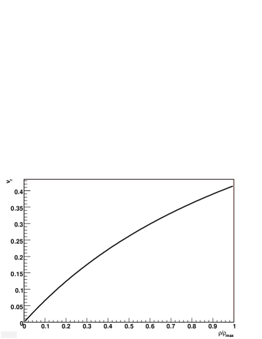
Figure 1: Radial velocity profile for the parameters used in this study.

Figure 2: Probability to emit a pion (green triangles), kaon (blue squares) and proton (red circles) as a function of time.

Table 1: Average emission times from Therminator

Particle species	Average emission time
pion	12.3 $fm/c$
kaon	10.7 $fm/c$
proton	7.9 $fm/c$

The simulation proceeds as follows. First, using a Monte-Carlo integration procedure as a particle generator, all particles (stable and unstable) are generated according to the emission function (10). Each particle is given an emission point on the freeze-out hypersurface and a momentum. Then all unstable particles decay after some random time dependent on their width. They propagate to the decay point, and this point is taken as the space-time origin of the daughter particles. Two- and three-particle decays are implemented. The process is repeated for cascade decays, until only stable particles remain. While each particle has emission point on the freeze-out hypersurface (we call such particles primordial) or at the decay point of the heavier resonance, the full history of decays can be reconstructed from the output files. This treatment of resonance propagation and decay is of crucial importance for non-identical particle correlations. It introduces delay in emission time, different for different particle species. It depends on the number of resonances that decay into the particle of interest, their widths and velocities. An illustration can be seen on Fig. 2. The Monte-Carlo procedure we used is the most efficient way of studying it, more precise results can only be obtained by using a full-fledged hadronic rescattering model. In our work hadronic rescattering is not taken into account, which is one of the simplifications assumed in the single freeze-out model.

IV.1 Calculating the correlation function

It is possible to use Eq. 2 to get the model correlation function. The integral is calculated numerically. One takes particles generated by Therminator. Then one combines them into pairs and creates two histograms - in one of them one stores the squared wave-function of the pair (4), in the other - unity for each pair. The result of the division of the two histograms is the average pair wave function in each bin, which is the correlation function per Eq. (2). This is the so-called “two-particle weight” method of calculating the correlation function from models. It is the only one which enables to take into account the two-particle Coulomb interaction exactly, a feature which is necessary for our study. In the procedure each pair is treated separately, for each of them one goes to the pair rest frame (different for each pair) as the calculation of the pair wave function is done most naturally in this system.

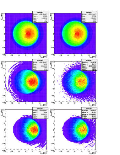
Figure 3: Distribution of emission points of pions (upper plots), kaons (center plots) and protons (lower plots) versus pair-wise out and side directions. Left and right side are emission points of the same particle from different system, but the same pair velocity range (for pions: left - $\pi K$, right - $\pi p$, for kaons: left - $\pi K$, right - $Kp$, for protons: left - $\pi p$, right - $Kp$

V Asymmetry analysis

In section III it was shown that non-identical particle correlations are sensitive to the shifts between average emission points of different particle species. However we have not discussed if and how such asymmetries could arise. In Fig. 3 average emission points of pions, kaons and protons from THERMINATOR where shown, for pairs which have similar velocity, pointing horizontally to the right. One sees right away that the average emission points of pions, kaons and protons is not the same in the $out$ direction, while it is 0 for the side direction for all of them. One can also see that the average size of the emission region is decreasing with particle mass, a known effect of radial flow, usually referred to as the “$m_{T}$ scaling” of HBT radii. The shift that we observe is also a direct but distinctly different consequence of radial flow present in our simulation. One can understand it by the following argument. Close velocity pions and protons have very different momenta. By inspecting Eq. (10) one observes that the correlation between space-momentum emission point direction $\phi$ and momentum direction $\varphi$ is controlled by the factor: $\exp(\beta p_{\perp}\cos(\varphi-\phi))$. So the higher the momentum, the stronger the correlation. Temperature $1/\beta$ is of course identical for both particle species. Therefore, in a close-velocity pair, proton emission direction will be much more correlated with its momentum direction. And the momentum, due to radial flow, is always pointing “outward”, so the emission points will tend to be concentrated near the edge of the system, in the direction of emission. For pions on the other hand, there is almost no correlation between the two directions, so they are emitted from the whole source. This is clearly seen in the figure, as a difference between mean emission points in the “out” direction:

$$r^{\pi p}_{out}=x^{\pi}_{out}-x^{p}_{out}$$ (11)

This is the spatial shift between particles in the source frame. Measuring it is the main goal of non-identical particle femtoscopy. Observing such shift in the experiment would be a direct evidence of the collective behaviour of matter, which is one of the necessary conditions to claim the discovery of the quark-gluon plasma.

One must remember that the asymmetries measured in the correlation function are averaged over the source. Therefore the connection between shift in laboratory frame and pair rest frame is:

$$\left<r^{*}_{out}\right>=\left<\gamma\left(r_{out}-\beta\Delta t\right)\right>$$ (12)

Table 2: Average space shifts from Therminator

$\beta_{t}$ of the pair	$r_{\pi K}$	$r_{\pi p}$	$r_{Kp}$
0.35 - 0.5	-1.9 fm	-2.5 fm	-0.6 fm
0.5 - 0.65	-2.4 fm	-3.4 fm	-0.9 fm
0.65 - 0.8	-2.9 fm	-3.9 fm	-1.1 fm
0.8 - 0.95	-3.0 fm	-4.3 fm	-1.2 fm

Table 3: Average time shifts from Therminator

$\beta_{t}$ of the pair	$\Delta t_{\pi K}$	$\Delta t_{\pi p}$	$\Delta t_{Kp}$
0.35 - 0.5	3.8 fm/c	6.2 fm/c	2.3 fm/c
0.5 - 0.65	3.6 fm/c	5.7 fm/c	2.1 fm/c
0.65 - 0.8	3.2 fm/c	5.1 fm/c	1.9 fm/c
0.8 - 0.95	2.6 fm/c	4.2 fm/c	1.5 fm/c

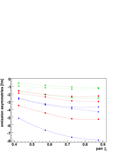
Figure 4: Components of the average shift between particle species in the laboratory frame. Dotted line is space component, dash-dotted line is time component, dashed line is full asymmetry. Red circles is $\pi K$ system, blue triangles is $\pi p$, green squares is $Kp$.

From Eq. (8) one sees that the measurable shift $r^{*}_{out}$ is a combination of spatial shift $r_{out}$, and emission time shift $\Delta t$. The former effect is of special interest and has been studied in detail in LisaRetiere . However the effect of time difference has not been adequately studied so far. The Therminator model has been chosen to perform this task, because it includes both effects in the same calculation in a self-consistent way. Fig. 2 shows the probability to emit a pion, a kaon or a proton at a given time. One sees that average emission times of this particle species, listed in Tab. 1, are different in the laboratory frame. This will affect the observed asymmetries.

In Fig. 4 one can see the components of the emission asymmetries in the laboratory frame, obtained directly from the emission functions $S_{1,2}$. The time and space components for all considered systems are compared. They are of the same order for all systems. The overall asymmetry is the combination of the two.

V.1 Obtaining femtoscopic information

The correlation function for non-identical particles is given by Eq. (2). In order to obtain femtoscopic information from the experimental correlation function one needs to perform a fit procedure. In traditional HBT measurement the integral analog to Eq. (2) can be performed analytically to obtain a simple fit function. It is not possible for the general case of non-identical particles, where the following procedure must be applied. Usually smoothness approximation is used, that is the emission function factorizes into a space and momentum components. A form of the spatial emission function is then assumed:

$$S(\vec{r})\approx exp\left(-\frac{(r_{out}-\mu_{out})^{2}+r_{side}^{2}+r_{long}^{2}}{2R^{2}}\right)$$ (13)

defined in the laboratory frame. Then momenta of pairs of particles are taken from the experiment. Their emission points are randomly generated according to (13), with some assumed values of source parameters: the gaussian source radius $R$ and the shift in the outwards direction $\mu_{out}$. For each pair the weight is then calculated according to (4), and the average of the weights over all pairs as a function of $k^{*}$ is constructed. This is a theoretical correlation function according to (2). This function can be compared via a $\chi^{2}$ test to the experimental correlation function being fitted. By varying parameters $R$ and $\mu_{out}$ a function can be found which best describes the input one. Parameters of the source which produce this function are taken as the best-fit values. In this way femtoscopic information is obtained from the non-identical particle correlation function. In this work the model correlation functions calculated according to Eq. 2 were treated as “pseudo-experimental” ones. A dedicated program Kisiel:2004phd ; Kisiel:Nukl has been used to perform a fit on them in a manner as closely resembling the experimental situation as possible. It was a direct test of the methodology of non-identical particle correlations.

V.2 Sum rule for shifts between different particle species

If we have three different particle species, we have three average emission point shifts that we can measure: $\mu^{\pi K}$, $\mu^{\pi p}$ and $\mu^{Kp}$. However, if we take the same group of e.g. pions for $\pi-K$ correlations and $\pi-p$ correlations (and similarly the same group of kaons and protons), we might expect that a simple sum rule holds:

$$\mu^{\pi p}=\mu^{\pi K}+\mu^{Kp}$$ (14)

and only two of the shifts are independent.

Non-identical particles are correlated if they have close velocities. If we select pairs of particles with some pair velocity, we expect that the correlated particles themselves also have velocities in this range. Therefore if we compare pions that form the $\pi-K$ correlation in the pair $\beta_{t}$ range between 0.5 and 0.65, and pions from the $\pi-p$ correlation in the same pair $\beta_{t}$ range we may assume that these are the same pions (providing that we construct the correlation functions from the same events). That shows that pair $\beta_{t}$ is the correct variable to select on, when studying momentum dependence of the femtoscopic parameters from non-identical particle correlations. It also shows that we should indeed expect the sum rule (14) to hold separately in each $\beta_{t}$ bin.

V.3 Two-particle versus single particle sizes

The size of the two-particle source is a combination of the individual single-particle source sizes:

$$\sigma_{\pi K} = \sqrt{\sigma_{\pi}^{2}+\sigma_{K}^{2}}$$

$$\sigma_{\pi p} = \sqrt{\sigma_{\pi}^{2}+\sigma_{p}^{2}}$$

$$\sigma_{Kp} = \sqrt{\sigma_{K}^{2}+\sigma_{p}^{2}}$$ (15)

where $\sigma$ is a width of a gaussian fitted to the corresponding emission function (either single- or two-particle). One can immediately see that the sizes are not independent, similar to shifts. One can also use the combination of the measured two-particle source sizes to obtain the single particle sizes:

$$\sigma_{\pi} = \sqrt{\frac{\sigma_{\pi K}^{2}+\sigma_{\pi p}^{2}-\sigma_{Kp}^{2}}{2}}$$

$$\sigma_{K} = \sqrt{\frac{\sigma_{\pi K}^{2}-\sigma_{\pi p}^{2}+\sigma_{Kp}^{2}}{2}}$$

$$\sigma_{p} = \sqrt{\frac{-\sigma_{\pi K}^{2}+\sigma_{\pi p}^{2}+\sigma_{Kp}^{2}}{2}}$$ (16)

They can then be compared to single-particle source sizes obtained from regular identical particle interferometry to see whether the size of the system is described self-consistently.

VI Results and discussion

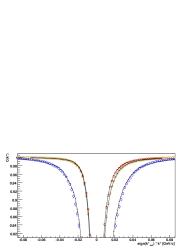
Figure 5: Correlation functions for pion-kaon (red), pion-proton (yellow) and kaon-proton (blue) for pairs with velocity between 0.5 and 0.65. The lines are fits to the correlation function.

The analysis of the correlation functions for pion-kaon, pion-proton and kaon-proton systems has been performed based on the Therminator model and the two particle weight method, described in the previous paragraphs. Examples of the obtained correlation functions are shown in Fig. 5. As expected for like-sign pairs they go below unity at low $k^{*}$. The correlation effect is the smallest for pion-kaon and largest for kaon-proton due to the difference in the Bohr radii of the pairs. It is a fortunate coincidence, as for kaon-proton one expects to have the smallest statistics in the experiment, but due to a large correlation effect the measurement should be doable for a data sample similar to the one in which pion-kaon measurement is possible.

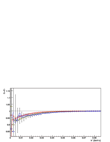
Figure 6: Double ratios for pion-kaon (red), pion-proton (yellow) and kaon-proton (blue) for pairs with velocity between 0.5 and 0.65. The lines are double ratios calculated from the fits to the correlation function.

In Fig. 6 examples of the asymmetry measurement - the double ratios $C_{+}/C_{-}$ for pion-kaon, pion-proton and kaon-proton systems, are shown. One can see a significant signal, which indicates that the correlation functions are indeed sensitive to the asymmetries described in the previous paragraph. In our analysis we have adopted a convention in which a lighter particle is always taken as first in the pair. All the double ratios go below unity, which means that, on average, particles which are lighter are emitted closer to the center of the system or later (or both). This is exactly consistent with the qualitative picture of spatial shifts coming from radial flow shown in Fig. 3 and with emission time differences coming from resonance decays, shown in Fig. 2 and Tab. 3.

The correlation functions have been fitted using the numerical Monte-Carlo procedure described in Sect. IV. Fig. 5 shows the resulting best-fit functions as solid lines. The fit is performed simultaneously to the positive $k^{*}_{out}$ and negative $k^{*}_{out}$ part of the correlation function. The lines in Fig. 6 are simply the two parts of the fit function from Fig. 5 divided by each other, they are not fit independently.

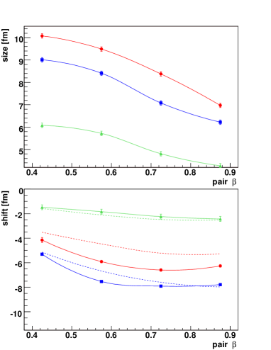
Figure 7: Parameters of the non-identical particle sources from fits. In the upper panel source size is shown, in the lower - shift between mean emission points in the direction of pair transverse momentum. Red circles are for pion-kaon, Blue squares for pion-proton, green triangles for kaon-proton. Dashed lines are input overall asymmetries from Fig. 4

The results of the fit are shown in Fig. 7. We find that the size of the emitting system decreases with pair velocity for all considered pair types. This is consistent with the “$m_{T}$ scaling” of the HBT radii observed in the identical particle femtoscopy calculations. The shifts between various particle species have an expected ordering - the larger the mass difference, the larger the shift. This means that for all observed systems the lighter particle is emitted, on the average, closer to the center and/or later than the heavier one. It also means that time differences do not change the qualitative behaviour of the observed asymmetries. However, consulting Tab. 3 and Fig. 4, one can see that they do contribute to the observed asymmetry. The dashed lines in Fig. 7 show the overall asymmetry from Fig. 4 as predicted directly from the emission functions $S_{1,2}(\mathbb{r})$ from the model. The agreement in absolute values and general trends between them and the final fit values is within $1.0fm$.

This is of crucial importance for the experiment. It means that by performing an advanced fit of all three combinations of non-identical particle correlation functions one can indeed infer the properties of the underlying two-particle emission functions, and therefore obtain a new, unique piece of information about the dynamics of the collision.

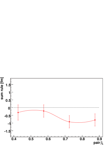
Figure 8: Test of the sum rule of mean shifts between various particle types.

One can also test the validity of the sum rule (14). The test using the fit values from Fig. 7 is shown in Fig. 8. One can see that the rule is valid for smaller pair velocity and holds only approximately for larger velocities. This should be compared to results in Tab. 2, where the shifts obtained from the separation distributions themselves follow the sum rule with the accuracy of $0.1fm$. Also one can expect deviations on the order of the differences between the input and fitted values of the shift shown in Fig. 7. One can see that within these systematic limits the agreement is acceptable. This is another important conclusion for the experiment. If shifts between all three combinations are measured in the comparable pair velocity window one expects the sum rule for the shifts (14) to hold. It can be used as a quality check on the data.

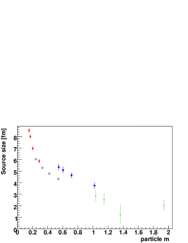
Figure 9: Single particle source sizes obtained from non-identical particle correlation fits, according to (16). Red circles are pions sizes, blue squares - kaon, green triangles - proton. Open circles are sizes obtained from identical-particle $\pi$ correlations.

One can also use the fitted two-particle radii for all systems to obtain the single particle radii according to (16). The results are shown in Fig. 9. The radii are reasonable and exhibit the expected “$m_{T}$ scaling” for all particle species. Therefore an experiment can extract the information not only about the asymmetries of emission but also about the size of the system. The comparison between the size estimates obtained from non-identical particle correlations and “HBT radii” obtained from identical pion interferometry was done. Both sizes for pions are consistent with each other. One must remember that in the case of Therminator model, the obtained source functions exhibit large long-range non-gaussian tails Kisiel:2006is . On the other hand, both identical and non-identical femtoscopic sizes were obtained assuming perfect gaussian source. Both of these measures can be sensitive to long-range tails in a different way, so the comparison must be done with caution.

VII Summary

We have presented the first complete set of calculations of non-identical particle correlations from the single freeze-out models with complete treatment of resonances. The non-identical particle femtoscopy method was shown to be sensitive to both the size and emission asymmetries in the system. The observed effects have been shown to be under control both qualitatively and quantitatively. The method to extract femtoscopic information from such correlation functions have been presented and employed to the “pseudo-experimental” functions obtained from the model. The results of the fit have been shown to be in agreement with the characteristics of the input source. Several consistency checks on the experimental data have been proposed and their validity tested. A method to test the consistency of identical and non-identical femtoscopy results has also been proposed.

The femtoscopic analysis of non-identical particle correlations has shown that the emission asymmetries between pions, kaons and protons are expected to occur in heavy-ion collisions. Spatial asymmetry coming from radial flow was observed. Time asymmetry coming from resonance propagation and decay was also estimated and found to be on the order of the space asymmetry in the laboratory frame and in the same direction for all tested systems. Therefore a realistic and self-consistent estimate of the two effects has been given for the first time. Consistency between identical and non-identical femtoscopic sizes was tested and found to be within 1.0 fm.

Predictions for both the size of the system as well as emission asymmetry has been given for the central AuAu collisions for pion-kaon, pion-proton and kaon-proton correlations.

Acknowledgements

This work was supported by Polish Ministry of Science and Higher Education, grants no. 0395/P03/2005/29 and 134/E-365/SPB/CERN/P-03/DWM 97/2004-2007. I would like to thank prof. W. Broniowski and prof. W. Florkowski for very fruitful discussions.

References

- (1) W. Florkowski, W. Broniowski and M. Michalec, “Thermal analysis of particle ratios and p(T) spectra at RHIC,” Acta Phys. Polon. B 33, 761 (2002) [arXiv:nucl-th/0106009].
- (2) W. Broniowski and W. Florkowski, “Explanation of the RHIC p(T)-spectra in a thermal model with expansion,” Phys. Rev. Lett. 87, 272302 (2001) [arXiv:nucl-th/0106050].
- (3) W. Broniowski, A. Baran and W. Florkowski, “Thermal model at RHIC. II: Elliptic flow and HBT radii,” AIP Conf. Proc. 660, 185 (2003) [arXiv:nucl-th/0212053].
- (4) A. Kisiel, W. Florkowski and W. Broniowski, “Femtoscopy in hydro-inspired models with resonances,” Phys. Rev. C 73, 064902 (2006) [arXiv:nucl-th/0602039].
- (5) J. Adams et al. [STAR Collaboration], “Pion kaon correlations in Au + Au collisions at s(NN)**(1/2) = 130-GeV,” Phys. Rev. Lett. 91, 262302 (2003) [arXiv:nucl-ex/0307025].
- (6) F. Retiere and M. A. Lisa, “Observable implications of geometrical and dynamical aspects of freeze-out in heavy ion collisions,” Phys. Rev. C 70, 044907 (2004) [arXiv:nucl-th/0312024].
- (7) R. Lednicky, V.L. Lyuboshitz, Yad. Fiz. 35 (1982) 1316 (Sov. J. Nucl. Phys. 35 (1982) 770); Proc. Int. Workshop on Paricle Correlations and Interferometry in Nuclear Collisions, CORINNE 90, Nantes, France 1990 (ed. D. Ardouin, World Scientific 1990) p. 42; Heavy Ion Physics 3 (1996) 1
- (8) R. Lednicky, V. L. Lyuboshits, B. Erazmus and D. Nouais, “How to measure which sort of particles was emitted earlier and which later,” Phys. Lett. B 373, 30 (1996).
- (9) S. Voloshin, R. Lednicky, S. Panitkin and N. Xu, “Relative space-time asymmetries in pion and nucleon production in noncentral nucleus nucleus collisions at high energies,” Phys. Rev. Lett. 79, 4766 (1997) [arXiv:nucl-th/9708044].
- (10) R. Lednicky, “Finite-size effects on two-particle production in continuous and discrete spectrum,” arXiv:nucl-th/0501065.
- (11) A. Kisiel, “Non-identical particle femtoscopy in heavy-ion collisions,” AIP Conf. Proc. 828, 603 (2006).
- (12) A. Kisiel, “Studies of non-identical meson-meson correlation at low relative velocities in relativistic heavy-ion collisions registered in the STAR experiment”, PhD Thesis, Warsaw Univeristy of Technology, Dec 2004
- (13) A. Kisiel, T. Taluc, W. Broniowski and W. Florkowski, “THERMINATOR: Thermal heavy-ion generator,” Comput. Phys. Commun. 174, 669 (2006) [arXiv:nucl-th/0504047].
- (14) S. Eidelman et al. [Particle Data Group], “Review of particle physics,” Phys. Lett. B 592, 1 (2004).
- (15) J. Adams et al. [STAR Collaboration], “Pion, kaon, proton and anti-proton transverse momentum distributions from p + p and d + Au collisions at s(NN)**1/2 = 200-GeV,” Phys. Lett. B 616, 8 (2005) [arXiv:nucl-ex/0309012].
- (16) A. Kisiel, “CorrFit - a program to fit arbitrary two-particle correlation functions” NUKLEONIKA 2004, 49(Supplement 2):s81-s83