Nuclear Superfluidity in Exotic Nuclei and Neutron Stars

Abstract

Nuclear superfludity in exotic nuclei close to the drip lines and in the inner crust matter of neutron stars have common features which can be treated with the same theoretical tools. In the first part of my lecture I discuss how two such tools, namely the HFB approach and the linear response theory can be used to describe the pairing correlations in weakly bound nuclei, in which the unbound part of the energy spectrum becomes important. Then, using the same models, I shall discuss how the nuclear superfluidity can affect the thermal properties of the inner crust of neutron stars.

1 Introduction

The basic features of nuclear superfluidity are the same in finite nuclei and in infinite Fermi systems such as neutron stars. Yet, in atomic nuclei the pairing correlations have special features related to the finite size of the system. The way how the finite size affects the pairing correlations depends on the position of the chemical potential. If the chemical potential is deeply bound, like in stable and heavy nuclei, the finite size influences the pairing correlations mainly through the shell structure induced by the spin-orbit interaction. The situation becomes more complex in weakly bound nuclei close to the drip lines, where the chemical potential approaches the continuum threshold. In this case the inhomogeneity of the pairing field can produce a strong coupling between the bound and the unbound part of the single-particle spectrum. This is an issue which will be discussed in the first part of my lecture. More precisely, I shall discuss how the continuum coupling and the pairing correlations can be treated in the framework of the Hartree-Fock-Bogoliubov (HFB) approach and linear response theory.

The neutron-drip line put a limit to the neutron-rich nuclei which can be produced in the laboratory or in supernova explosions (via rapid neutron-cupture processes). However, this limit can be overpassed in the inner crust of neutron stars since there the driped neutrons are kept together with the neutron-rich nuclei by the gravitational preasure.

The superfluid properties of the inner crust have been considered long ago in connection with post-glitch timing observations and colling processes [1, 2, 3]. However, although the neutron star matter superfluidity has been intensively studied in the last decades [4], so far only a few microscopic calculations have been done for the superfluidity of inner crust matter. The most sophisticated microscopic calculations done till now use the framework of HFB approach at finite temperature [5]. They will be discussed in the second part of my lecture. The discussion will be focused on the effects induced by the pairing correlations on the specific heat and on the cooling time of the inner curst of neutron stars.

2 Pairing correlations in exotic nuclei

2.1 Continuum-HFB approach

The tool commonly used for treating pairing correlations in exotic nuclei close to the drip lines is the Hartree-Fock-Bogoliubov (HFB) approach [6]. The novel feature of interest here is how within this approach one can treat properly the quasiparticle states belonging to the continuum spectrum [7]. This issue is discussed below.

The HFB equations for local fields and spherical symmetry have the form:

$$\begin{array}[]{c}\left(\begin{array}[]{cc}h(r)-\lambda&\Delta(r)\\ \Delta(r)&-h(r)+\lambda\end{array}\right)\left(\begin{array}[]{c}U_{i}(r)\\ V_{i}(r)\end{array}\right)=E_{i}\left(\begin{array}[]{c}U_{i}(r)\\ V_{i}(r)\end{array}\right)~{},\end{array}$$ (1)

where $\lambda$ is the chemical potential, $h(r)$ is the mean field hamiltonian and $\Delta(r)$ is the pairing field. The fields depend on particle density $\rho(r)$ and pairing density $\kappa(r)$ given by:

$$\rho(r)=\frac{1}{4\pi}\sum_{i}(2j_{i}+1)V_{i}^{*}(r)V_{i}(r),$$ (2)

$$\kappa(r)=\frac{1}{4\pi}\sum_{i}(2j_{i}+1)U_{i}^{*}(r)V_{i}(r).$$ (3)

In the calculations presented here the mean field is described with a Skyrme force and for the pairing interaction it is used a density- dependent force of zero range of the following form [8]:

$$V(\mathbf{r}-\mathbf{r^{\prime}})=V_{0}[1-\eta(\frac{\rho}{\rho_{0}})^{\alpha}]\delta(\mathbf{r}-\mathbf{r^{\prime}})\equiv V_{eff}(\rho(r))\delta(\mathbf{r}-\mathbf{r^{\prime}}).$$ (4)

For this force the pairing field is given by $\Delta(r)=\frac{V_{eff}}{2}\kappa(r)$.

The HFB equations have two kind of solutions. Thus, between 0 and $-\lambda$ the quasiparticle spectrum is discrete and both upper and lower components of the radial HFB wave function decay exponentially at infinity. On the other hand, for $E>-\lambda$ the spectrum is continuous and the solutions are:

$$u_{lj}(E,r) = C[cos(\delta_{lj})j_{l}(\alpha_{1}r)-sin(\delta_{lj})n_{l}(\alpha_{1}r)]~{},$$

$$v_{lj}(E,r) = D_{1}h_{l}^{(+)}(i\beta_{1}r)~{},$$ (5)

where $j_{l}$ and $n_{l}$ are spherical Bessel and Neumann functions repectively and $\delta_{lj}$ is the phase shift corresponding to the angular momentum $(lj)$. The phase shift is found by matching the asymptotic form of the wave function written above with the inner radial wave function. From the energy dependence of the phase shift one can determine the energy regions of quasiparticle resonant states. In HFB they are of two types. A first type corresponds to the single-particle resonances of the mean field. A second kind of resonant states is specific to the HFB approach and corresponds to the bound single-particle states which in the absence of pairing correlations have an energy $\epsilon<2\lambda$. Among all possible resonances, of physical interest are the ones close to the continuum threshold. An exemple of such resonances is shown in section 2.4.

2.2 Resonant states in the BCS approach

The low-lying quasiparticle resonances can be also calculated in the framework of the BCS approach. The BCS approximation is obtained by neglecting in the HFB equations the non-diagonal matrix elements of the pairing field. This means that in the BCS limit one neglects the pairing correlations induced by the pairs formed in states which are not time-reversed partners.

The extension of BCS equations for taking into account the effect of resonant states was proposed in Refs.[9, 10]. For the case of a general pairing interaction the corresponding resonant-BCS equations read [9]:

$$\Delta_{i}=\sum_{j}V_{i\overline{i}j\overline{j}}u_{j}v_{j}+\sum_{\nu}V_{i\overline{i},\nu\epsilon_{\nu}\overline{\nu\epsilon_{\nu}}}\int_{I_{\nu}}g_{\nu}(\epsilon)u_{\nu}(\epsilon)v_{\nu}(\epsilon)d\epsilon~{},$$ (6)

$$\Delta_{\nu}\equiv\sum_{j}V_{\nu\epsilon_{\nu}\overline{\nu\epsilon_{\nu}},j\overline{j}}u_{j}v_{j}+\sum_{\nu^{\prime}}V_{\nu\epsilon_{\nu}\overline{\nu\epsilon_{\nu}},\nu^{\prime}\epsilon_{\nu^{\prime}}\overline{\nu^{\prime}\epsilon_{\nu^{\prime}}}}\int_{I_{\nu^{\prime}}}g_{\nu^{\prime}}(\epsilon^{\prime})u_{\nu^{\prime}}(\epsilon^{\prime})v_{\nu^{\prime}}(\epsilon^{\prime})d\epsilon^{\prime}~{},$$ (7)

$$N=\sum_{i}v_{i}^{2}+\sum_{\nu}\int_{I_{\nu}}g_{\nu}(\epsilon)v^{2}_{\nu}(\epsilon)d\epsilon~{}.$$ (8)

Here $\Delta_{i}$ is the gap for the bound state $i$ and $\Delta_{\nu}$ is the averaged gap for the resonant state $\nu$. The quantity $g_{\nu}(\epsilon)=\frac{2j_{\nu}+1}{\pi}\frac{d\delta_{\nu}}{d\epsilon}$ is the continuum level density and $\delta_{\nu}$ is the phase shift of angular momentum $(l_{\nu}j_{\nu})$. The factor $g_{\nu}(\epsilon)$ takes into account the variation of the localisation of scattering states in the energy region of a resonance ( i.e., the width effect) and becomes a delta function in the limit of a very narrow width. In these equations the interaction matrix elements are calculated with the scattering wave functions at resonance energies and normalised inside the volume where the pairing interaction is active.

The BCS equations written above have been solved with a single particle spectrum corresponding to a HF [9] and a RMF [11] mean field. It was shown that by including in the BCS equations a few relevant resonances close to the continuum threshold one can get results very similar to the ones obtained in the HFB and RHB calculations. One can thus conclude that in nuclei close to the dripline the quasiparticle spectrum is dominated by a few low-lying resonances. In many odd-even nuclei close to the drip lines these low-lying quasiparticle resonances might be the only measurable excited states. Their widths can be calculated from the phase shift behaviour or from the imaginary part of the energies associated to the Gamow states [12].

In even-even nuclei the low-lying quasiparticle resonances could form the main component of unbound collective excitations with a finite time life. How these excitations can be treated in nuclei close to the drip line is discussed in the next section.

2.3 Linear response theory with pair correlations and continuum coupling

The collective excitations of atomic nuclei in the presence of pairing correlations is usually described in the Quasiparticle-Random Phase Approximation (QRPA) [6]. In nuclei characterized by a small nucleon separation energy, the excited states are strongly influenced by the coupling with the quasiparticle continuum configurations. Among the configurations of particular interest are the two-quasiparticle states in which one or both quasiparticles are in the continuum. In order to describe such excited states one needs a proper treatment of the continuum coupling, which is missing in the usual QRPA calculations based on a discrete quasiparticle spectrum. In this section we discuss how the pairing and the continuum coupling can be treated in the framework of the linear response theory [13, 14].

The response of the nuclear system to an external perturbation is obtained from the time-dependent HFB equations (TDHFB) [6]:

$$i\hbar\frac{\partial{\cal R}}{\partial t}=[{\cal H}(t)+{\cal F}(t),{\cal R}(t)],$$ (9)

where ${\cal R}$ and ${\cal H}$ are the time-dependent generalized density and the HFB Hamiltonian, respectively. ${\cal F}$ is the external oscillating field :

$${\cal F}=Fe^{-i\omega t}+h.c..$$ (10)

In Eq. (10) $F$ includes both particle-hole and two-particle transfer operators :

$$F=\sum_{ij}F^{11}_{ij}c_{i}^{\dagger}c_{j}+\sum_{ij}(F^{12}_{ij}c_{i}^{\dagger}c_{j}^{\dagger}+F^{21}_{ij}c_{i}c_{j}),$$ (11)

and $c_{i}^{\dagger}$, $c_{i}$ are the particle creation and annihilation operators, respectively.

In the small amplitude limit the TDHFB equations become:

$$\hbar\omega{\cal R}^{\prime}=[{\cal H}^{\prime},{\cal R}^{0}]+[{\cal H}^{0},{\cal R}^{\prime}]+[F,{\cal R}^{0}],$$ (12)

where the superscript  ’ stands for the corresponding perturbed quantity.

The variation of the generalized density ${\cal R}$’ is expressed in term of 3 quantities, namely $\rho^{\prime}$, $\kappa^{\prime}$ and $\bar{\kappa}^{\prime}$, which are written as a column vector :

$$\rho^{\prime}=\left(\begin{array}[]{c}\rho^{\prime}\\ \kappa^{\prime}\\ \bar{\kappa}^{\prime}\\ \end{array}\right),$$ (13)

where $\rho^{\prime}_{ij}=\left<0|c^{\dagger}_{j}c_{i}|^{\prime}\right>$ is the variation of the particle density, $\kappa^{\prime}_{ij}=\left<0|c_{j}c_{i}|^{\prime}\right>$ and $\bar{\kappa}^{\prime}_{ij}=\left<0|c^{\dagger}_{j}c^{\dagger}_{i}|^{\prime}\right>$ are the fluctuations of the pairing tensor associated to the pairing vibrations and $\mid^{\prime}\rangle$ denotes the change of the ground state wavefunction $|0>$ due to the external field.

The variation of the HFB Hamiltonian is given by:

$${\cal H}^{\prime}=\bf{V}\rho^{\prime},$$ (14)

where $\bf{V}$ is the matrix of the residual interaction expressed in terms of the second derivatives of the HFB energy functional, namely:

$${\bf{V}}^{\alpha\beta}({\bf r}\sigma,{\bf r}^{\prime}{\sigma}^{\prime})=\frac{\partial^{2}{\cal E}}{\partial{\bf{\rho}}_{\beta}({\bf r}^{\prime}{\sigma}^{\prime})\partial{\bf{\rho}}_{\bar{\alpha}}({\bf r}\sigma)},~{}~{}~{}\alpha,\beta=1,2,3.$$ (15)

In the above equation the notation $\bar{\alpha}$ means that whenever $\alpha$ is 2 or 3 then $\bar{\alpha}$ is 3 or 2.

Introducing for the external field the three dimensional column vector:

$$\bf{{F}}=\left(\begin{array}[]{c}{F}^{11}\\ {F}^{12}\\ {F}^{21}\\ \end{array}\right),$$ (16)

the density changes can be written in the standard form:

$${\rho^{\prime}}=\bf{G}\bf{F}~{}\boldmath,$$ (17)

where $\bf{G}$ is the QRPA Green’s function obeying the Bethe-Salpeter equation:

$$\bf{G}=\left(1-\bf{G}_{0}\bf{V}\right)^{-1}\bf{G}_{0}=\bf{G}_{0}+\bf{G}_{0}\bf{V}\bf{G}.$$ (18)

The unperturbed Green’s function $\bf{G}_{0}$ has the form:

$${\bf{G}_{0}}^{\alpha\beta}({\bf r}\sigma,{\bf r}^{\prime}{\sigma}^{\prime};\omega)=\sum_{ij}\int\hskip 8.5359pt\frac{{\cal U}^{\alpha 1}_{ij}({\bf r}\sigma)\bar{{\cal U}}^{*\beta 1}_{ij}({\bf r}^{\prime}\sigma^{\prime})}{\hbar\omega-(E_{i}+E_{j})+i\eta}-\frac{{\cal U}^{\alpha 2}_{ij}({\bf r}\sigma)\bar{{\cal U}}^{*\beta 2}_{ij}({\bf r}^{\prime}\sigma^{\prime})}{\hbar\omega+(E_{i}+E_{j})+i\eta},$$ (19)

where $E_{i}$ are the qp energies and ${\cal U}_{ij}$ are 3 by 2 matrices expressed in term of the two components of the HFB wave functions [13]. The $\sum$ $\int$   symbol in Eq. (19) indicates that the summation is taken over the discrete and the continuum quasiparticle states.

The QRPA Green’s function can be used for calculating the strength function associated with various external perturbations. For instance, the transitions from the ground state to the excited states induced by a particle-hole external field can be described by the strength function:

$$S(\omega)=-\frac{1}{\pi}Im\int F^{11*}({\bf r}){\bf{G}}^{11}({\bf r},{\bf r}^{\prime};\omega)F^{11}({\bf r}^{\prime})d{\bf r}~{}d{\bf r}^{\prime}$$ (20)

where ${\bf{G}}^{11}$ is the (ph,ph) component of the QRPA Green’s function. Another process which can be described in the same manner is the two-particle transfer from the ground state of a nucleus with A nucleons to the excited states of a nucleus with A+2 nucleons. For this process the strength function is:

$$S(\omega)=-\frac{1}{\pi}Im\int F^{12*}({\bf r}){\bf{G}}^{22}({\bf r},{\bf r}^{\prime};\omega)F^{12}({\bf r}^{\prime})d{\bf r}~{}d{\bf r}^{\prime}$$ (21)

where ${\bf{G}}^{22}$ denotes the (pp,pp) component of the Green’s function.

2.4 Quasiparticle excitations and two-neutron transfer in neutron-rich nuclei

The formalisms presented above are illustrated here for the case of neutron-rich oxygen isotopes [13, 14]. First, we present an exemple of quasiparticle resonances calculated in the framework of the continuum-HFB (cHFB) approach introduced in section 3.1. In the cHFB calculations the mean field quantities are evaluated using the Skyrme interaction SLy4 [17], while for the pairing interaction we take a zero-range density-dependent force. The parameters of the pairing force are given in Ref [13]. The HF single-particle and HFB quasiparticle energies corresponding to the $sd$ shell and to the $1f_{7/2}$ state are listed in Table 1. One can notice that in both HF and cHFB calculations the state $1f_{7/2}$ is a wide resonance for ^18-22O nuclei, while the state $1d_{3/2}$ is a narrow resonance. As seen below, these one-quasiparticle resonances determine essentially the two-quasiparticle states which are the stongest populated in even-even oxygen isotopes.

Table 1. HF and HFB energies in oxygen isotopes.

		18O	20O	22O
1d5/2	HF	-6.7	-7.0	-7.45
1d5/2	cHFB	2.26	2.08	2.30
2s1/2	HF	-4.0	-4.2	-4.6
2s1/2	cHFB	3.46	2.28	1.05
1d3/2	HF	(0.46;0.02)	(0.51;0.03)	(0.42;0.02)
1d3/2	cHFB	(7.74;0.12)	(6.60;0.29)	(5.39;0.01)
1f7/2	HF	(5.50;1.35)	(5.24;1.24)	(4.86;1.04)
1f7/2	cHFB	(12.77;1.13)	(12.14;0.83)	(10.05;0.69)

The two-quasiparticle states are calculated by using the response theory described in section 2.3. In the calculations one includes the full discrete and continuum HFB spectrum up to 50 MeV. These states are used to construct the unperturbed Green’s function ${\bf G_{0}}$. After solving the Bethe-Salpeter equation for the QRPA Green function one constructs the strength functions written in section 2.3. The details of the calculations can be found in Ref[14]. Here we show the results obtained for the collective states excited in the two-neutron transfer. The strength function corresponding to a neutron pair transferred to the oxygen isotope ²²O is shown in Fig.1.

Figure 1: The response function for the two-neutron transfer on 22O. The unperturbed response is in solid line and the QRPA response in dashed line.

For the isotope ²²O the subshell $d_{5/2}$ is essentially blocked for the pair transfer. Therefore in this nucleus we can clearly identify only two peaks below 11 MeV, corresponding to a pair transferred to the states $2s_{1/2}$ and $2d_{3/2}$. The strength function shown in Fig. 1 shows also a broad peak around 20 MeV. This peak is built mainly upon the single-particle resonance $1f_{7/2}$ and its cross section is much larger than the one associated to the lower energy transfer modes. Since this high energy transfer mode is formed mainly by single-particle states above the valence shell, this mode is similar to the giant pairing vibration mode suggested long ago [15]. Although such a mode has not been detected yet, the pair transfer reactions involving exotic loosely bound nuclei may offer a better chance for this undertaking [16].

3 Superfluid and thermal properties of neutron stars crust

In this section we analyse the superfluid properties of a nuclear system in which the limit of the neutron-drip line is overpassed: the inner crust of neutron stars. The inner crust consists of a lattice of neutron-rich nuclei immersed in a sea of unbound neutrons and relativistic electrons. Down to the inner edge of the crust, the crystal lattice is most probably formed by spherical nuclei. More inside the star, before the nuclei dissolve completely into the liquid of the core, the nuclear matter can develop other exotic configurations as well, i.e, rods, plates, tubes, and bubbles [18]. The thickness of the inner crust is rather small, of the order of one kilometer, and its mass is only about 1$\%$ of the neutron star mass. However, in spite of its small size, the properties of inner crust matter, especially its superfluid properties, have important consequences for the dynamics and the thermodynamics of neutron stars. In what follows we will discuss the main features of the pairing correlations inside the inner crust matter. Then we shall focus on the effects induced by the nuclear superfluidity on the specific heat and on the cooling time of the curst.

3.1 Superfluid properties of the inner crust matter

The superfluid properties of the inner crust matter discussed here [5] are based on the finite-temperature HFB (FT-HFB) approach. For zero range forces and spherical symmetry the radial FT-HFB have a similar form as the HFB equations at zero temperature, ie.,

$$\begin{array}[]{c}\left(\begin{array}[]{cc}h_{T}(r)-\lambda&\Delta_{T}(r)\\ \Delta_{T}(r)&-h_{T}(r)+\lambda\end{array}\right)\left(\begin{array}[]{c}U_{i}(r)\\ V_{i}(r)\end{array}\right)=E_{i}\left(\begin{array}[]{c}U_{i}(r)\\ V_{i}(r)\end{array}\right)~{},\end{array}$$ (22)

where $E_{i}$ is the quasiparticle energy, $U_{i}$, $V_{i}$ are the components of the radial FT-HFB wave function and $\lambda$ is the chemical potential. The quantity $h_{T}(r)$ is the thermal averaged mean field hamiltonian and $\Delta_{T}(r)$ is the thermal averaged pairing field. The latter depends on the average pairing density $\kappa_{T}$. In a self-consistent calculation based on a Skyrme-type force , $h_{T}(r)$ is expressed in terms of thermal averaged densities, i.e., kinetic energy density $\tau_{T}(r)$, particle density $\rho_{T}(r)$ and spin density $J_{T}(r)$, in the same way as in the Skyrme-HF approach. The thermal averaged densities mentioned above are given by [5]:

$$\rho_{T}(r)=\frac{1}{4\pi}\sum_{i}(2j_{i}+1)[V_{i}^{*}(r)V_{i}(r)(1-f_{i})\\ +U_{i}^{*}(r)U_{i}(r)f_{i}]$$

$$\kappa_{T}(r)=\frac{1}{4\pi}\sum_{i}(2j_{i}+1)U_{i}^{*}(r)V_{i}(r)(1-2f_{i})$$

$$J_{T}(r) = \frac{1}{4\pi}\sum_{i}(2j_{i}+1)[j_{i}(j_{i}+1)-l_{i}(l_{i}+1)-\frac{3}{4}]$$

$$\times\{V_{i}^{2}(1-f_{i})+U_{i}^{2}f_{i}\}$$

$$\tau_{T}(r) = \frac{1}{4\pi}\sum_{i}(2j_{i}+1)\{[(\frac{dV_{i}}{dr}-\frac{V_{i}}{r})^{2}+\frac{l_{i}(l_{i}+1)}{r^{2}}V_{i}^{2}]$$

$$\times(1-f_{i})+[(\frac{dU_{i}}{dr}-\frac{U_{i}}{r})^{2}+\frac{l_{i}(l_{i}+1)}{r^{2}}U_{i}^{2}]f_{i}\},$$

where $f_{i}=[1+exp(E_{i}/k_{B}T)]^{-1}$ is the Fermi distribution, $k_{B}$ is the Boltzmann constant and T is the temperature. The summations in the equations above are over the whole quasiparticle spectrum, including the unbound states.

The FT-HFB equations are solved for the spherical Wigner-Seitz cells determined in Ref.[20]. To generate far from the nucleus a constant density corresponding to the neutron gas, the FT-HFB equations are solved by imposing Dirichlet-Neumann boundary conditions at the edge of the cell [20], i.e., all wave functions of even parity vanish and the derivatives of odd-parity wave functions vanish. In the FT-HFB calculations we use for the particle-hole channel the Skyrme effective interaction SLy4 [17], which has been adjusted to describe properly the mean field properties of neutron-rich nuclei and infinite neutron matter. In the particle-particle channel we employ a density dependent zero range force. Since the magnitude of pairing correlations in neutron matter is still a subject of debate, the parameter of the pairing force are chosen so as to describe two different scenarios for the neutron matter superfluidity. Thus, for the first calculation we use the parameters: $V_{0}$=-430 MeV fm³, $\eta$=0.7, and $\alpha$=0.45. With these parameters and with a cut-off energy for the quasiparticle spectrum equal to 60 MeV one obtains approximately the pairing gap given by the Gogny force in nuclear matter [8]. In the second calculation we reduce the strength of the force to the value $V_{0}$=-330 MeV fm³. With this value of the strength we simulate the second scenario for the neutron matter superfluidity, in which the screening effects would reduce the maximum gap in neutron matter to a value around 1 MeV [21].

The FT-HFB results are shown here for two representative Wigner-Seitz cells chosen from Ref.[20]. These cells contain Z=50 protons and have rather different baryonic densities, i.e., 0.0204 fm^-3 and 0.00373 fm^-3. The cells, which contain N=1750 and N=900 neutrons, respectively, are denoted below as a nucleus with Z protons and N neutrons, i.e., ¹⁸⁰⁰Sn and ⁹⁵⁰Sn. The FT-HFB calculations are done up to a maximum temperature of T=0.5 MeV, which is covering the temperature range of physical interest [22].

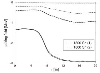
Figure 2: Neutron pairing fields for the cell ¹⁸⁰⁰Sn calculated at various temperatures. The numbers 1 and 2 which follow the cell symbol (see the inset) indicate the variant of the pairing force used in the calculations. The full and the dashed lines corresponds (from bottom upwards) to the set of temperatures T=$\{0.0,0.5\}$ MeV and T=$\{0.0,0.1,0.3,0.5\}$MeV, respectively.

The temperature dependence of the pairing fields in the two cells presented above is shown in Figs.2-3. First, we notice that for all temperatures the nuclear clusters modify significantly the profile of the pairing field. One can also see that for most of the cases the temperature dependence of the pairing field is significant. This is clearly seen in the low-density cell ⁹⁵⁰Sn.

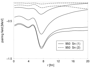
Figure 3: The same as in Fig.1, but for the cell ⁹⁵⁰Sn. The full and the dashed lines corresponds (from bottom upwards) to the set of temperatures T=$\{0.0,0.1,0.3,0.5\}$ and T=$\{0.0,0.1\}$MeV, respectively

3.2 Specific heat of the inner crust baryonic matter

The superfluid properties of the neutrons discussed in the previous section have a strong influence on the specific heat of the inner crust matter [5]. The specific heat of a given cell of volume V is defined by:

$$C_{V}=\frac{1}{V}\frac{\partial\mathcal{E}(T)}{\partial T},$$ (24)

where $\mathcal{E}(T)$ is the total energy of the baryonic matter inside the cell, i.e.,

$$\mathcal{E}(T)=\sum_{i}f_{i}E_{i}.$$ (25)

Due to the energy gap in the excitation spectrum, the specific heat of a superfluid system is dramatically reduced compared to its value in the normal phase. Since the specific heat depends exponentially on the energy gap, its value for a Wigner-Seitz cell is very sensitive to the local variations of the pairing field induced by the nuclear clusters. This can be clearly seen in Fig.4, where the specific heat is plotted for the cell ¹⁸⁰⁰Sn and for the neutrons uniformly distributed in the same cell. One can notice that at T=0.1 MeV and for the first pairing force the presence of the cluster increases the specific heat by about 6 times compared to the value for the uniform neutron gas. However, the most striking fact seen in Fig.4 is the huge difference between the predictions of the two pairing forces. Thus, for T=0.1 MeV this difference amounts to about 7 orders of magnitude.

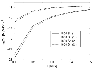
Figure 4: Specific heat for the cell ¹⁸⁰⁰Sn as a function of temperature. The notations used in the inset and the representation of the calculated values are the same as in Figs.1-3.

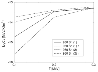
Figure 5: The same as in Fig.4, but for the cell ⁹⁵⁰Sn.

The behaviour of the specific heat for the low- density cell ⁹⁵⁰Sn is shown in Fig.5. For the first pairing force we can also see that at T=0.1 MeV the cluster increases the specific heat by about the same factor as in the cell ¹⁸⁰⁰Sn. However, for the second pairing force the situation is opposite: the presence of the nucleus decreases the specific heat instead of increasing it.

3.3 Collective modes in the inner crust matter

In the calculations presented in the previous section the specific heat of inner crust matter was evaluated by considering only non-interacting quasiparticles states. However, the specific heat can be also strongly affected by the collective modes created by the residual interaction between the quasiparticles, especially if these modes appear at low-excitation energies.

The collective modes in the inner crust matter were calculated in Ref. [23] in the framework of linear response theory discussed in section 2.3. The most important result of these calculations is the apparence of very collective modes at low energies, of the order of the pairing gap. An example of such mode is seen in Fig.6, were is shown the quadrupole response for the cell ¹⁸⁰⁰Sn. As can be clearly seen from Fig.6 , when the residual interaction is introduced among the quasiparticles the unperturbed spectrum, distributed over a large energy region, is gathered almost entirely in the peak located at about 3 MeV. This peak collects more than 99$\%$ of the total quadrupole strength and is extremely collective. An indication of the extreme collectivity of this low-energy mode can be also seen from its reduced transition probability, B(E2), which is equal to 25.10³ Weisskopf units. This value of B(E2) is two orders of magnitude higher than in standard nuclei. This underlines the fact that this WS cell cannot be simply considered as a giant nucleus. The reason is that in this cell the collective dynamics of the neutron gas dominates over the cluster contribution.

Figure 6: Quadrupole strength distribution of neutrons for the cell ¹⁸⁰⁰Sn. The full curve represents the QRPA strength, and the dashed line is the HFB unperturbed strength.

The collective excitations located at low energies can affect significantly the specific heat of the inner crust baryonic matter. This can be seen in Fig.7, where the specific heat corresponding to the collective modes (of multipolarity L=0,1,2,3) is shown. We notice that for T=0.1 MeV the specific heat given by the collective modes is of the same order of magnitute as the one corresponding to HFB spectrum. Therefore one expects that the collective modes of the inner crust matter could affect strongly the thermal behaviour of the crust.

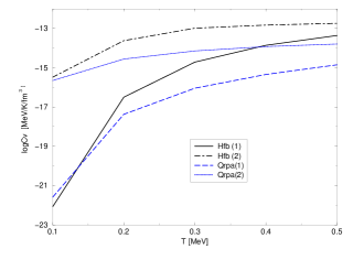
Figure 7: Specific heat in the cell ¹⁸⁰⁰Sn. The dashed line corresponds to the collective modes and the full line to the HFB spectrum

3.4 Cooling time of the inner crust

The specific heat of the inner crust matter is an important quantity for cooling time calculations. In this section we shall discuss the sensivity of the cooling time on the specific heat calculated with the two scenarios for the nuclear superfluidity introduced in section 3.1. The cooling process we analyse here corresponds to a fast cooling mechanism (e.g., induced by direct Urca reactions). In this case the interior of the star cools much faster than the crust. The cooling time is defined as the time needed for the cooling wave to traverse the crust and to arrive at the surface of the star. According to numerical simulations [24], the cooling time is proportional to the square of the crust size and to the specific heat. This result was used by Pizzochero et al [25] for estimating the cooling time in a simple model, which we have also employed in our calculations [26]. Thus, the crust is devided in shells of thickness $R_{i}$ for which the thermal difusivity $D_{i}$ could be considered as constant. Then the cooling time is obtained by summing the contribution of each shell, i.e.,

$$t_{cool}=\frac{1}{\gamma}\sum_{i}\frac{R_{i}^{2}}{D(i,T)}$$ (26)

The thermal diffusivity is given by $D=\frac{\kappa}{C_{V}}$, where $\kappa$ is the thermal conductibility and $C_{V}$ is the specific heat. The thermal conductivity is mainly determined by the electrons and in our calculations we have used the values reported by Lattimer et al. [24]. The specific heat $C_{V}$ has major contributions from the electrons, which can be easily calculated, and from the neutrons of the inner crust. As we have seen above, the specific heat of the neutrons depends strongly on pairing correlations. In order to see if this dependence has observationally consequences for the cooling time, we have performed two calculations, corresponding to the strong and the weak pairing forces introduced in section 3.1. The calculations show that the cooling time is increasing with more than $80\%$ if for calculating the pairing correlations we use a weak pairing force instead of a strong pairing force. This result indicates that the nuclear superfluidity of the inner crust matter plays a crucial role for the cooling time calculation of neutron stars.

4 Conclusions

In this lecture we have shown how the HFB approach and the linear response theory can be used to describe the pairing correlations in exotic nuclei and in the inner crust of neutron stars. Thus, for the nuclei close to the drip lines we have discussed how one can incorporate in the two approaches mentioned above the effects of the continuum coupling on pairing correlations. Then, using the same models, we have analysed what are the effects of pairing correlations on the specific heat and on the cooling time of neutron stars. We thus found that the cooling time depends very strongly on the intensity of pairing correlations in nuclear matter. Because the intensity of pairing correlations in nuclear matter is still unclear, at present one can only estimate the limits in which the cooling time of the inner crust can vary. Since the pairing correlations in nuclear matter and in nuclei are in fact correlated, one hopes that these limits could be reduced by systematic studies of pairing in both infinite and finite nuclear systems.

References

- [1] D. Pines and M. Ali Alpar, Nature (London) 316, 27 (1985)
- [2] J. A. Sauls, in Timing Neutron Stars, ed. by H. Ogelman and E. P. J. van den Heuvel (Dordrecht, Kluwer, 1989) pp. 457
- [3] M. Prakash, Phys. Rep. 242 387 (1994);
- [4] U. Lombardo and H-J. Schulze, in Physics of Neutron Star Interiors, ed. by D.Blaschke et al (Springer,2001) pp.30
- [5] N. Sandulescu, Phys. Rev. C 70 025801
- [6] P. Ring, P. Schuck, The nuclear many-body problem, Springer-Verlag (1980).
- [7] M. Grasso, N. Sandulescu, Nguyen Van Giai, and R. J. Liotta, Phys. Rev. C64 064321 (2001)
- [8] G. F. Bertsch and H. Esbensen, Ann. Phys. (N.Y.) 209 327 (1991)
- [9] N. Sandulescu, N. Van Giai, and R.J. Liotta, Phys. Rev. C 61 061301(R) (2000)
- [10] N. Sandulescu, R. J. Liotta and R. Wyss, Phys. Lett. B394 6 (1997)
- [11] N. Sandulescu, L. S. Geng, H. Toki, and G. C. Hillhouse, Phys. Rev. C 68 054323 (2003)
- [12] R. Id. Betan, N. Sandulescu, T. Vertse, Nucl. Phys. A771 93 (2006)
- [13] E. Khan, N. Sandulescu, M. Grasso, Nguyen Van Giai, Phys. Rev C66 (2002) 024309.
- [14] E. Khan, N. Sandulescu, Nguyen Van Giai, M. Grasso, Phys. Rev. C69 (2004) 014314
- [15] M. W. Herzog, R. J. Liotta and T. Vertse Phys. Lett. B165 (1985) 35.
- [16] L. Fortunato, W. von Oertzen, H. M. Sofia and A. Vitturi, Eur. Phys. J. A14 (2002) 37.
- [17] E. Chabanat, P. Bonche, P. Haensel, J. Meyer, R. Schaeffer, Nucl. Phys. A635 231 (1998)
- [18] C. J. Pethick and D. G. Ravenhall, Annu. Rev. Nucl. Part. Sci. 45 429 (1995)
- [19] N. Sandulescu, Nguyen Van Giai, and R. J. Liotta, Phys. Rev. C69 045802 (2004)
- [20] J. W. Negele and D. Vautherin, Nucl. Phys. A207 298 (1973)
- [21] C. Shen, U. Lombardo, P. Schuck, W. Zuo, and N. Sandulescu, Phys. Rev. C67 061302R (2003)
- [22] K. A. van Riper, Ap.J. 75 449 (1991)
- [23] E. Khan, N. Sandulescu and Nguyen Van Giai, Phys. Rev. C71 042801 (2005)
- [24] J. M. Lattimer et al, ApJ 425 802 (1994)
- [25] P. M. Pizzochero, F. Barranco, E. Vigetti, and R. A. Broglia, ApJ 569 (2002) 381
- [26] J. Margueron, C. Monrozeau, N. Sandulescu, in preparation