Properties of the largest fragment in multifragmentation: a canonical thermodynamic calculation

Abstract

Many calculations for the production of light and intermediate particles resulting from heavy ion collisions at intermediate energies exist. Calculations of properties of the largest fragment resulting from multifragmentation are rare. In this paper we compute these properties and compare them with the data for the case of gold on carbon. We use the canonical thermodynamic model. The model also gives a bimodal distribution for the largest fragment in a narrow energy range.

I Introduction

The statistical model of nuclear disassembly in heavy ion collisions is quite successful. Here one assumes that the disintegrating system with a given excitation energy expands to greater than normal volume before it breaks up into many composites of various sizes. Interactions between different composites in the rarefied situation can be neglected and the break up can be calculated using the laws of equilibrium thermodynamics. This basic assumption is implemented in different versions according to degrees of sophistication and detail. Thus we have the statistical multifragmentation model (SMM) of Copenhagen Bondorf , the microcanonical model of Gross Gross and Randrup and Koonin Randrup . An easily implementable canonical ensemble model was later introduced Dasgupta1 . The details of the model and many applications can be found in a recent publication Das .

It has been customary to pay a great deal of attention to the production cross-sections of intermediate mass fragments and light charged particles. Here we study the properties of the largest fragment that emerges in multifragmentation. These properties are not easy to study but the canonical model allows for such computation. As we will see, the heaviest fragment also reveals some interesting physics. Data on the heaviest fragment and fragments with the maximum charge were published by EOS collaboration EOS1 ; EOS2 ; EOS3 . In these experiments one studied the disintegrations of projectile-like excited fragments in the reactions Au+C, La+C and Kr+C. We do our calculations for Au+C. Calculations for the other two systems will be similar.

In section II we write down the theoretical formulae needed for the calculations. Results are presented in section III. Summary and conclusions are presented in section IV.

II Formulae in the canonical model

The formulae used in this calculation are provided here. Simpler formulae for a hypothetical system of one kind of particles are given in Das .

We will consider disassembly of the projectile-like fragment(PLF) where the PLF is formed by the shearing off of a part of ¹⁹⁷Au (by the ¹²C target). This PLF will have a charge $Z$ (usually less than 79) and a neutron number $N$ (usually less than 118). This PLF will break up into many composites with charges $i$ and neutron number $j$ (for example, ⁹Be has $i=4$ and $j=5$). If the number of composite with proton and neutron numbers $i$ and $j$ respectively is $n_{i,j}$ then conservation of charge and baryon number dictates that $Z=\sum i\times n_{i,j}$ and $N=\sum j\times n_{i,j}$.

The canonical partition function for the system at a given temperature $T$ is given in our model by

$$Q_{Z,N}=\sum\prod\frac{\omega_{i,j}^{n_{i,j}}}{n_{i,j}!}$$ (1)

Here the sum is over all possible channels of break-up (the number of such channels is enormous) which satisfies the conservation laws; $\omega_{i,j}$ is the partition function of one composite with proton number $i$ and neutron number $j$ respectively and $n_{i,j}$ is the number of this composite in the given channel. This is a low-density/ high temperature approximation the justification of which is demonstrated in Jennings and Das . For a given channel the sum $\sum_{i,j}n_{i,j}$ is called the multiplicity of the channel. The one-body partition function $\omega_{i,j}$ is a product of two parts: one arising from the translational motion of the composite and another from the intrinsic partition function of the composite:

$$\omega_{i,j}=\frac{V_{f}}{h^{3}}(2\pi m(i+j)T)^{3/2}\times z_{i,j}(int)$$ (2)

Here $m(i+j)$ is the mass of the composite and $V_{f}$ is the volume available for translational motion; $V_{f}$ will be less than $V$, the volume to which the system has expanded at break up. We use $V_{f}=V-V_{0}$ , where $V_{0}$ is the normal volume of the PLF. We will shortly discuss the choice of $z_{i,j}(int)$ used in this work.

The probability of a given channel $P(\vec{n}_{i,j})\equiv P(n_{0,1},n_{1,0},n_{1,1}......n_{i,j}.......)$ is given by

$$P(\vec{n}_{i,j})=\frac{1}{Q_{Z,N}}\prod\frac{\omega_{i,j}^{n_{i,j}}}{n_{i,j}!}$$ (3)

The average number of composites with $i$ protons and $j$ neutrons is seen easily from the above equation to be

$$\langle n_{i,j}\rangle=\omega_{i,j}\frac{Q_{Z-i,N-j}}{Q_{Z,N}}$$ (4)

The constraints $Z=\sum i\times n_{i,j}$ and $N=\sum j\times n_{i,j}$ can be used to obtain different looking but equivalent recursion relations for partition functions. For example

$$Q_{Z,N}=\frac{1}{Z}\sum_{i,j}i\omega_{i,j}Q_{Z-i,N-j}$$ (5)

Instead of labelling partition functions by their charge and neutron numbers $Z$ and $N$ we can for example label them by total mass ($A\equiv Z+N$) and charge $Z$. Labelling them by $\tilde{Q}$ we have

$$\tilde{Q}_{A,Z}=\frac{1}{A}\sum_{a,i}a\tilde{\omega}_{a,i}\tilde{Q}_{A-a,Z-i}$$ (6)

These recursion relations allow one to calculate $Q_{Z,N}$ (equivalently $\tilde{Q}_{A,Z}$) very quickly in the computer.

We list now the properties of the composites used in this work. The proton and the neutron are fundamental building blocks thus $z_{1,0}(int)=z_{0,1}(int)=2$ where 2 takes care of the spin degeneracy. For deuteron, triton, ³He and ⁴He we use $z_{i,j}(int)=(2s_{i,j}+1)\exp(-\beta e_{i,j}(gr))$ where $\beta=1/T,e_{i,j}(gr)$ is the ground state energy of the composite and $(2s_{i,j}+1)$ is the experimental spin degeneracy of the ground state. Excited states for these very low mass nuclei are not included. For mass number $A=5$ and greater we use the liquid-drop formula. For nuclei in isolation, this reads ($a=i+j$)

$$z_{i,j}(int)=\exp\frac{1}{T}[W_{0}a-\sigma(T)a^{2/3}-\kappa\frac{i^{2}}{a^{1/3}}-s\frac{(i-j)^{2}}{a}+\frac{T^{2}a}{\epsilon_{0}}]$$ (7)

The derivation of this equation is given in several places Bondorf ; Das so we will not repeat the arguments here. The expression includes the volume energy, the temperature dependent surface energy, the Coulomb energy, the symmetry energy and contribution from excited states since the composites are at a non-zero temperature. For $i,j$, (the proton and the neutron number) we include a ridge along the line of stability. We have used two sets to test the sensitivity of the results to the width of of the ridge. We call these set 1 and set 2. In set 1 for each $a$ between 5 and 40, 5 isotopes are included (case for $a$=4 and lower was already mentioned before); For $a>40$, 7 isotopes are included for each $a$. In set 2, 5 isotopes are used for $a$ between 5 and 9, 7 isotopes are used for $a$ between 10 and 40 and 9 isotopes for each $a>40$. The results are quite similar in most cases except for one figure which we will point out when we compare with data. It should be pointed out that enlarging the width of the ridge does not necessarily imply a better calculation as one may begin to overcount the phase space.

The Coulomb interaction is long range. The Coulomb interaction between different composites can be included in an approximation called the Wigner-Seitz approximation. We incorporate this following the scheme set up in Bondorf . This requires adding in the argument of the exponential of Eq.(7) a term $\kappa\frac{i^{2}}{a^{1/3}}(V_{0}/V)^{1/3}(\frac{Z_{0}/A_{0}}{i/a})^{1/3}$. Here $A_{0},Z_{0}$ are the mass and charge number respectively of the disintegrating system, $V_{0}$ is the normal nuclear volume for this system and $V$, the freeze-out volume (typically 4-5 times $V_{0}$). Defining $R_{f}^{3}\equiv\frac{3V}{4\pi}$ the energy of the system is given by $E=\frac{3Z_{0}^{2}}{5R_{f}}+\sum_{i,j}\langle n_{i,j}\rangle e_{i,j}$ where for $a>4$ we have $e_{i,j}=\frac{3}{2}T+a(-W_{0}+T^{2}/\epsilon_{0})+\sigma(T)a^{2/3}+\kappa\frac{i^{2}}{a^{1/3}}[1.0-(V_{0}/V)^{1/3}(\frac{Z_{0}/A_{0}}{i/a})^{1/3}]+s\frac{(i-j)^{2}}{a^{2}}-T[\partial\sigma(T)/\partial T]a^{2/3}$. For $a\leq 4$ we use $e_{i,j}=\frac{3}{2}T+e_{i,j}(gr)-\kappa\frac{i^{2}}{a^{1/3}}(V_{0}/V)^{1/3}(\frac{Z_{0}/A_{0}}{i/a})^{1/3}$. We label as $E^{*}$ the excitation energy: $E^{*}=E-E(gr)$ where $E(gr)$ is calculated for mass number $A_{0}$ and charge $Z_{0}$ using the liquid-drop formula.

The central issue in this work is the calculation of $\langle Z_{max}\rangle$ and $\langle A_{max}\rangle$ (and their fluctuations) when the fragmenting system has charge $Z_{0}$ and mass number $A_{0}$. Let us fix on calculating $\langle Z_{max}\rangle$. The calculation for $\langle A_{max}\rangle$ can be done by analogy with appropriate and obvious changes in the formulae. There is an enormous number of channels in Eq.(1). Different channels will have different values of $Z_{max}$. For example there is a term $\frac{\omega_{1,0}^{Z}}{Z!}\frac{\omega_{0,1}^{N}}{N!}$ in the sum of Eq.(1). In this channel $Z_{max}$ is 1. The probability of this channel occurring is (from Eq.(3)) $\frac{1}{Q_{Z,N}}\frac{\omega_{1,0}^{Z}}{Z!}\frac{\omega_{0,1}^{N}}{N!}$. The full partition function can be written as $Q_{Z,N}=Q_{Z,N}(\omega_{1,0},\omega_{0,1},\omega_{1,1},........\omega_{i,j}......)$. If we construct a $Q_{Z,N}$ where we set all $\omega$’s except $\omega_{1,0}$ and $\omega_{0,1}$ to be zero then this $Q_{Z,N}(\omega_{1,0},\omega_{0,1},0,0,0..............)=\frac{\omega_{1,0}^{Z}}{Z!}\frac{\omega_{0,1}^{N}}{N!}$ and this has $Z_{max}=1$. Consider now constructing a $Q(Z,N)$ with only three $\omega$’s: $Q_{Z,N}(\omega_{1,0},\omega_{0,1},\omega_{2,1},0,0,0,......)$. This will have $Z_{max}$ sometimes 1 (as $\frac{\omega_{1,0}^{Z}}{Z!}\frac{\omega_{0,1}^{N}}{N!}$ is still there) and sometimes 2 (as, for example, in the term $\frac{\omega_{2,1}^{3}}{3!}\frac{\omega_{1,0}^{Z-6}}{(Z-6)!}\frac{\omega_{0,1}^{N-3}}{N!}$).

We are now ready to write down a general formula. Let us ask the question: what is the probability that a given value $z_{m}$ occurs as the maximum charge? To obtain this we construct a $Q_{Z,N}$ where we set all values of $\omega_{z,j}=0$ when $z>z_{m}$. Call this $Q_{Z,N}(z_{m})$. Then $Q_{Z,N}(z_{m})/Q_{Z,N}$ (where $Q_{Z,N}$ is the full partition function with all the $\omega$’s) is the probability that the maximum charge is any value between 1 and $z_{m}$. Similarly we construct a $Q_{Z,N}(z_{m}-1)$ where $\omega_{z,j}$ is set at zero whenever $z>z_{m}-1$. The probability $p$ that $z_{m}$ is $Z_{max}$ is given by

$$p(z_{m})\equiv p(Z_{max}=z_{m})=\frac{Q_{Z,N}(z_{m})-Q_{Z,N}(z_{m}-1)}{Q_{Z,N}}$$ (8)

The average value of $Z_{max}$ at given temperature and for given $Z_{0},A_{0}$ is

$$Z_{max}=\sum_{z_{m}=1}^{z_{m}=Z_{0}}z_{m}p(z_{m})$$ (9)

and the fluctuation is

$$RMS(Z_{max})=\sqrt{\sum p(z_{m})(z_{m}-Z_{max})^{2}}$$ (10)

Before we end this section we want to mention that the largest composite we obtain at the end of the above calculation is at a finite temperature $T$ and can further decay by evaporation, ending up in a lower mass or charge number. From our past experience Das we know what the effect will be: $Z_{max}$ will decrease slightly but the effect on the $RMS(Z_{max})$ will be significant. Without the evaporation the calculated $RMS$ will be overestimated (see Fig.19 of Das ). Inclusion of evaporation as an after burner is not possible at this stage. The sum over $z_{m}$ (Eq.(9)) is too huge and for each $z_{m}$ there is a sum over neutron number. We will hope to get $Z_{max}$ nearly right but will overestimate the $RMS$ value. The next section compares data with our calculations.

III Decay of excited projectile-like fragmant

In the EOS experiment part of the projectile (Au, La and Kr) is sheared off by the ¹²C target. We will compare our calculations with the Au+C data. The size of the excited PLF which decays depends upon the impact parameter which also determines the amount of excitation energy per nucleon in the excited PLF. In Figs.1(b) and 1(c) of EOS1 the size of the excited PLF (the size and charge are denoted by $A_{0}$ and $Z_{0}$) is plotted as a function of excitation energy $E^{*}$ per nucleon. This aspect of the experiment depends upon dynamics and is outside the scope of a thermodynamic model. However, given $E^{*}$ and $A_{0},Z_{0}$, this excited PLF will expand and break up into many pieces and this is calculable in a canonical thermodynamic model. In our Fig.1 (data taken from Fig.1(f) of EOS1 ) we have plotted $Z_{max}/Z_{0}$ as a function of $E^{*}$ per nucleon where $Z_{max}$ is the average maximum charge carried by a composite. The data are shown as points joined by a dotted curve. The other curves are exploratory calculations. Our fit to experimental data is given in Fig.2. We now explain how the calculations are done.

For a given value of $A_{0},Z_{0}$, the experiment provides the value of $E^{*}$. The beginning of a canonical thermodynanic model besides $A_{0}$, $Z_{0}$, are a temperature and a freeze-out density $\rho/\rho_{0}$ (freeze-out density in unit of normal nuclear density $\rho_{0}$= 0.16fm^-3) which will then provide all the observables including $E^{*}$. For a fixed $E^{*}$ the canonical model employs a fixed $\rho/\rho_{0}$. For example, for central collisions of Sn on Sn at 50 Mev per nucleon beam energy, a freeze out density of one-sixth normal density gives good results for production cross-sections of intermediate mass fragments Das . However, in the EOS experiment $E^{*}$ varies over a wide range (from less than 2 MeV per nucleon where the validity of the thermodynamic model as used here can be questioned to 10 Mev per nucleon where the thermodynamic model is expected to work well) and hence we should expect that $\rho/\rho_{0}$ will also need to vary in this interval. In general, the freeze-out density will decrease as $M/A_{0}$ ($M$=multiplicity, $A_{0}$=mass number of the dissociating system) increases, reaching some asymptotic value for large multiplicity. In SMM Bondorf the freeze-out density varies in each channel, decreasing as the multiplicity increases (this makes Monte-Carlo simulation mandatory). In the canonical model, at a given temperature, the freeze-out density is kept fixed irrespective of channels. Thus the freeze-out density can be dependent only on the average multiplicity. Past comparisons with SMM predictions showed that at least for the obsrvables studied so far this simplification is quite adequate Tsang .

Fig.1 compares the data if in the calculation the freeze-out volume is kept fixed at $\rho/\rho_{0}$ =0.25 (a typical canonical model value) or at 0.39 (this is an often quoted value in the model used in EOS1 ; EOS2 ). The value 0.39 is clearly better at low values of $E^{*}$ but leaves too large a residue at higher $E^{*}$ whereas the value 0.25 is better at the higher end of $E^{*}$ but is an underestimation at the lower end of $E^{*}$. The data undoubtedly point to the need of a variable $\rho/\rho_{0}$ if the whole spectrum of $E^{*}$ is to be covered. In Fig.1, for brevity we show results with set 1 only (see previous section for the range of nuclei covered in set 1). Fig.2 compares data with our calculation where we use a variable $\rho/\rho_{0}$. We have used a parametrisation $\rho/\rho_{0}=a+b\exp(-c(E^{*}/A_{0}))$ where $a$=0.17, $b=0.83$ and $c=0.417$ MeV^-1. No optimisation of the fit was tried but the values are suitable for the low and high limits of $E^{*}$. Our values of $\rho/\rho_{0}$ are also very similar to those quoted in Table II of EOS3 where a different model was used. We have shown results with set 1 and set 2 (this includes a larger number of composites than set 1; see previous section).

In the canonical model calculation normally the inputs are the freeze-out density and temperature. Here we use the freeze-out density and $E^{*}$. Given this density and $E^{*}$ we find the temperature which would give back the $E^{*}$ we started with. We then calculate $Z_{max}$. Calculations for $A_{max}$ were also done and the fits are similar.

Next we turn to results for $\gamma_{2}$ and $RMS(Z_{max}/Z_{0})$ which are shown in Fig.3. Data are from Fig.2 of EOS1 . Here $\gamma_{2}=\frac{M_{2}M_{0}}{M_{1}^{2}}$ where $M_{k}$ is the $k$th moment of the fragment distribution: $M_{k}=\sum n_{a}a^{k}$. The over-estimation in the calculation for $RMS$ was already alluded to in the previous section. Afterburner for the largest fragment will bring the distribution more closely packed near the line of maximum stability thus reducing the fluctuation.

The probability distribution (Eq.8) of $Z_{max}$ as a function of $Z_{max}$ for EOS experiments is not known to us but in view of the recent interest in such distributions Gulminelli ; Pichon we have computed the distributions and displayed them in Fig.4. We find that there is a window where the distribution is bimodal. Usually for discussion of bimodality one uses a fixed freeze-out volume and varies the temperature but here, as we discussed before, our freeze-out density actually changes as $E^{*}$ (hence $T$) changes but the nature of bimodality is still clearly seen (if we fix the freeze-out density the plots are very similar). Probability distribution for $A_{max}$ (calculated but not shown here) also has the window for bimodality. Connection between bimodality and first order phase transition in the canonical model (which does have a first order phase transition) is being pursued and we also hope to do calculations for other experimental data.

IV Summary and Discussion

The canonical thermodynamic model clearly reproduces many important features of the largest fragment resulting from multifragmentation. The model is very easy to implement and yet is very realistic. The same model gives remarkable fits to light charged particles, intermediate mass fragments and as we have just seen, the largest fragment as well. We have thus far reported the calculation of properties of the largest fragment without making any link with the subject of liquid-gas phase transition. We make a brief connection here. In a large system(see details in a recent article Chaudhuri ) composites with charge $z\leq 20$ comprise the gas phase. At co-existence, there will be, in addition, one large composite which is the liquid. This picture gets blurred as the system size is reduced, but , nonetheless, the largest fragment (at temperatures below that which displays bimodality) is an approximate scaled down version of the liquid. In a finite system bimodality in the largest fragment distribution occurs in the temperature (energy) window where the system passes from the liquid-gas co-existence phase to the pure gas phase. The largest cluster has been discussed in the literature before Gulminelli ; Krishnamachari ; Pleimling ; Binder . However these all use the lattice gas model or the Ising model (often with fixed magnetisation). Our approach here is more directly related to nuclear physics phenomenology with phase transition issues in the background.

V Acknowledgement

This work is supported by the Natural Sciences and Engineering Research Council of Canada.

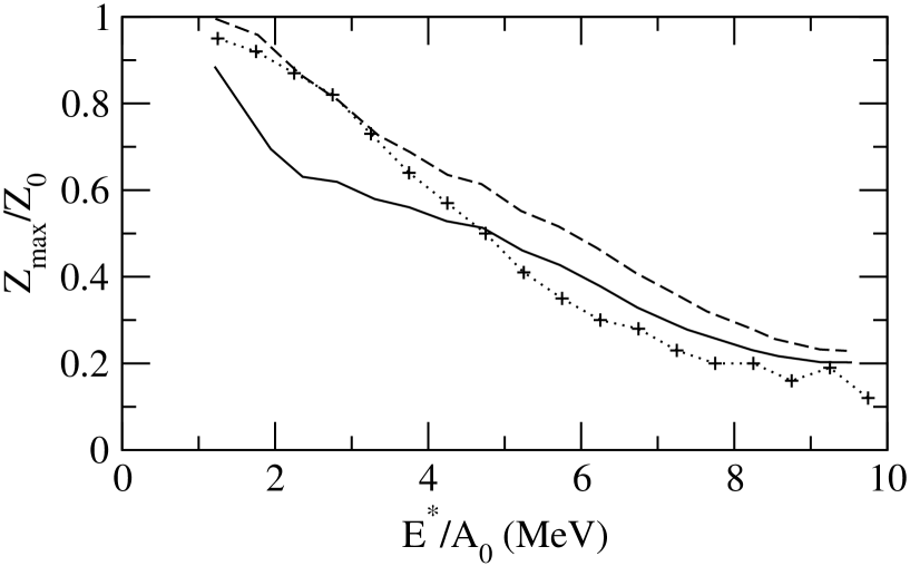
Figure 1: Experimental points (from Fig.1(f) of EOS1 ) are joined by a dotted line to guide the eye. The calculations are exploratory: these are done for a fixed freeze-out density (solid line for $\rho/\rho_{0}$=0.25 and dashed line for $\rho/\rho_{0}$=0.39). A higher freeze-out density produces a higher value of $\langle Z_{max}\rangle$. In the figures $Z_{max}$ stands for this average value. The calculations shown here include the composites of set 1. See the discussion following eq.(7) for enumeration of composites included in set 1 and set 2.

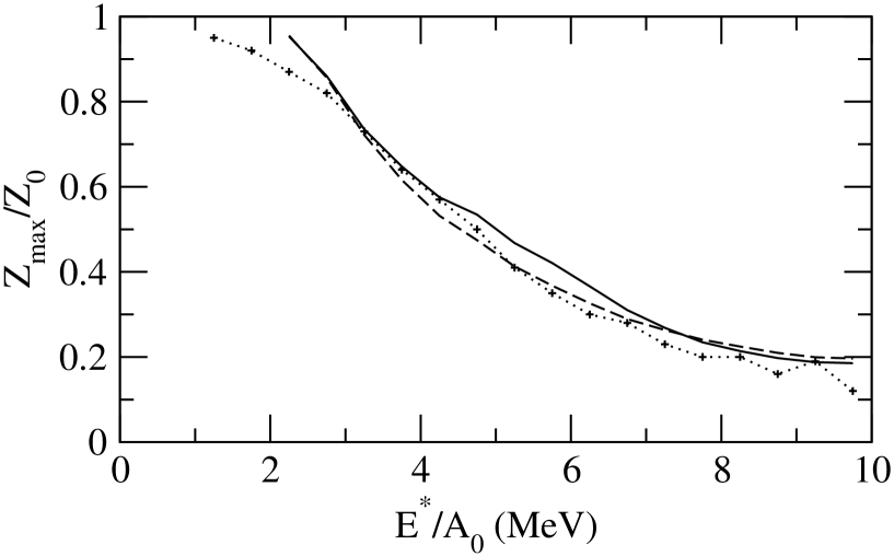
Figure 2: It is expected that the freeze-out density will decrease with excitation energy in this energy range. The calculations here use a parametrisation $\rho/\rho_{0}=a+b\exp(-c(E^{*}/A_{0}))$ where $a$=0.17, $b$=0.83 and $c$=0.417 MeV^-1. The solid line uses set 1, the dashed line uses set 2. Experimental data are joined by a dotted line.

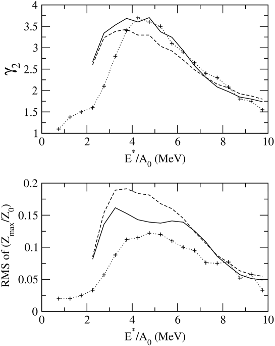
Figure 3: Top panel compares experimental data for $\gamma_{2}$ (fig.2 of EOS1 ) with calculations. For definition of $\gamma_{2}$, see the text. The solid curve uses set 1 and the dashed curve uses set 2. The bottom panel compares experimantal values of $RMS$ of $Z_{max}$ with the canonical calculation. As explained in the text, without an afterburner evaporation calculation, $RMS$ values from theory will significantly overestimate actual $RMS$. Evaporation will bring the population much closer to the line of maximum stability. For an estimate of effects of evaporation see fig.19 of Das . It is not surprising that with set 2 (dashed curve) calculated values of $RMS$ exceed those calculated with set 1. As more nuclei further from the line of maximum stability are included the effects of evaporation will be stronger.

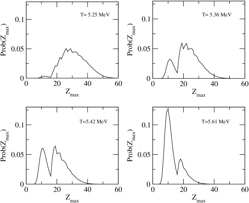
Figure 4: Theoretical values of the probablity of occurrence of a $Z_{max}$ plotted as a function of $Z_{max}$ (see eq.(8)). In a small window of $E^{*}$ (equivalently $T$ as shown here) a bimodal distribution is seen. Similar plot of probability of $A_{max}$ against $A_{max}$ also shows bimodality. The plots here use set 1

References

- (1) J. P. Bondorf, A. S. Botvina, A. S. Iljinov, I. N. Mishustin and K. Sneppen, Phys. Rep. 257, 133 (1995).
- (2) D. H. Gross, Phys. Rep. 279, 119 (1997).
- (3) J. Randrup, and S. E. Koonin, Nucl. Phys. A471, 355c (1987).
- (4) S. Das Gupta and A. Z. Mekjian, Phys. Rev. C57, 1361 (1998).
- (5) C. B. Das, S. Das Gupta, W. G. Lynch, A. Z. Mekjian, and M. B. Tsang, Phys. Rep. 406, 1 (2005).
- (6) J. B. Elliott et al., Phys. Rev. C 67, 024609 (2003).
- (7) J. A. Hauger et al., Phys. Rev. C 62, 024616 (2000).
- (8) J. A. Hauger et al., Phys. Rev. C 57, 764 (1998).
- (9) B. K. Jennings and S. Das Gupta, Phys. Rev. C 62, 014901 (2000).
- (10) M. B. Tsang et al., Phys. Rev. C 64, 054615 (2001).
- (11) F. Gulminelli and Ph. Chomaz, Phys. Rev. C 71, 054607 (2005).
- (12) M. Pichon et al., Nucl. Phys. A 779, 267 (2006).
- (13) G. Chaudhuri, S. Das Gupta, and M. Sutton, Phys. Rev. B 74, 174106 (2006).
- (14) B. Krishnamachari, J. McLean, B. Cooper, and J. Sethna, Phys. Rev. B 54, 8899 (1996).
- (15) M. Pleimling and W. Selke, J. Phys. A: Math. Gen. 33, L199 (2000).
- (16) K. Binder, Physica A 319, 99 (2003); M. Biskup et al, Physica A 327, 583 (2003)