No-Core shell model for $A=47$ and $A=49$

Abstract

We apply an ab-initio approach to the nuclear structure of odd-mass nuclei straddling ${}^{48}Ca$. Starting with the NN interaction, that fits two-body scattering and bound state data we evaluate the nuclear properties of $A=47$ and $A=49$ nuclei in a no-core approach. Due to model space limitations and the absence of 3-body interactions, we incorporate phenomenological terms determined by fits to $A=48$ nuclei in a previous effort. Our modified Hamiltonian produces reasonable spectra for these odd mass nuclei. In addition to the differences in single-particle basis states, the absence of a single-particle Hamiltonian in our no-core approach obscures direct comparisons with valence effective NN interactions. Nevertheless, we compare the fp-shell matrix elements of our initial and modified Hamiltonians in the harmonic oscillator basis with a recent model fp-shell interaction, the GXPF1 interaction of Honma, Otsuka, Brown and Mizusaki. Notable differences emerge from these comparisons. In particular, our diagonal two-body $T=0$ matrix elements are, on average, about 800-900keV more attractive. Furthermore, while our initial and modified NN Hamiltonian fp-shell matrix elements are strongly correlated, there is much less correlation with the GXPF1 matrix elements.

I Introduction

The low-lying levels of the A=47-49 nuclei have long been of experimental and theoretical interest. On the one hand, extensive experimental information about these nuclei is available [BUR95] -[ENDS] and, on the other hand, this is a suitable nuclear mass region for developing and testing effective fp-shell Hamiltonians. Numerous detailed spectroscopic calculations have been reported. For example, in Ref. [MZPC96] , using a shell model approach, Martinez-Pinedo, Zuker, Poves and Caurier have performed full fp-shell calculations for the A=47 and A=49 isotopes of Ca, Sc, Ti, V, Cr and Mn. They employed the KB3 interaction [KB3] with phenomenological adjustments and they performed complete diagonalizations to obtain very good agreement with the experimental level schemes, transition rates and static moments. Extensive discussions of fp-shell effective Hamiltonians and nuclear properties can be found in recent shell model review articles [BAB01] ; [OtsukaHMSU01] ; [DJDean04] ; [Caurier05] .

Our interest in these nuclei stems from our goal to extend the ab-initio no-core shell model (NCSM) applications to heavier systems than previously investigated. Until recently, the NCSM, which treats all nucleons on an equal footing, had been limited to nuclei up through $A=16$. However, in a recent paper [VPSN06] we reported the first NCSM results for ${}^{48}Ca$, ${}^{48}Sc$ and ${}^{48}Ti$ isotopes, with derived and phenomenological two-body Hamiltonians. These three nuclei are involved in double-beta decay of ${}^{48}Ca$, and the interest in developing nuclear structure models for describing them is also related to the need for accurate calculations of the nuclear matrix elements involved in this decay. Our first goals were to see the limitations of such an approach applied to heavier systems and how much improvement one can obtain by adding phenomenological two-body terms involving all nucleons. In brief, the results were the following [VPSN06] : i) one finds that the charge dependence of the bulk binding energy of eight A=48 nuclei is reasonably described with an effective Hamiltonian derived from CD-Bonn interactionMachl , while there is an overall underbinding by about 0.4 MeV/nucleon; ii) the resulting spectra are too compressed compared with experiment; iii) when isospin-dependent central terms plus a tensor interaction are added to the Hamiltonian, one achieves accurate total binding energies for eight A=48 nuclei and reasonable low-lying spectra for the three nuclei involved in double-beta decay. Only five input data were used to determine the phenomenological terms - the total binding of ${}^{48}Ca$, ${}^{48}Sc$, and ${}^{48}Ti$ along with the lowest positive and negative parity excitations of ${}^{48}Ca$.

In the present paper we extend our previous approach to the odd-A isotopes ${}^{47}Ca$, ${}^{49}Ca$, ${}^{47}Sc$ and ${}^{47}K$, which differ by one nucleon from ${}^{48}Ca$. One of our goals is to test whether the same modified effective Hamiltonian used for A=48 isotopes, is able to describe these odd-A nuclei. A particular feature of the spectroscopy of these odd nuclei is that the spin-orbit splitting gives rise to a sizable energy gap in the fp-shell between the $f_{7/2}$ and other orbitals ($p_{1/2}$, $p_{3/2}$, $f_{5/2}$) and we wanted to see if this feature is reproduced in the NCSM where we have no input single-particle energies. Also, in spite of the differences in frameworks with and without a core, we wanted to compare our initial and modified Hamiltonian with a recent fp-shell interaction, the GXPF1, developed by Honma, Otsuka, Brown and Mizusaki [HOB04] . We feel it is valuable to compare various fp-shell interactions in order to understand better their shortcomings and their regimes of applicability. From the comparison we present here, notable differences are evident. For example, our diagonal two-body T=0 matrix elements are more attractive and, while our initial and modified NN Hamiltonian fp-shell matrix elements are strongly correlated, there is much less correlation with the GXPF1 matrix elements. It is worth mentioning that our interaction and Honma et al. GXPF1 interactions were also tested recently within the framework of spectral distribution theory in Ref. [SDV06] and sizable differences were demonstrated.

Our paper is organized as follows: in Section 2 we give a short review of the NCSM approach and we refer the reader to the bibliography for more details. Section 3 is devoted to the presentation of our results. Binding energies, excitation spectra, single-particle characteristics, monopole matrix elements and matrix element correlations are discussed in subsections along with corresponding figures. In the last Section we present the conclusion and the outlook of our work.

II NO-CORE SHELL MODEL

The NCSM ZBV ; NB96 ; NB98 ; NB99 ; NCSM12 ; NCSM6 is based on an effective Hamiltonian derived from realistic “bare” interactions and acting within a finite Hilbert space. All $A$-nucleons are treated on an equal footing. The approach is both computationally tractable and demonstrably convergent to the exact result of the full (infinite) Hilbert space.

Initial investigations used two-body interactions ZBV based on a G-matrix approach. Later, we implemented a similarity transformation procedure based on Okubo’s pioneering work Vefftot to derive two-body and three-body effective interactions from realistic NN and NNN interactions.

Diagonalization and the evaluation of observables from effective operators created with the same transformations are carried out on high-performance parallel computers.

II.1 Effective Hamiltonian

For pedagogical purposes, we outline the ab initio NCSM approach with NN interactions alone and point the reader to the literature for the extensions to include NNN interactions. We begin with the purely intrinsic Hamiltonian for the $A$-nucleon system, i.e.,

$$H_{A}=T_{\rm rel}+{\cal V}=\frac{1}{A}\sum_{i<j}^{A}\frac{(\vec{p}_{i}-\vec{p}_{j})^{2}}{2m}+\sum_{i<j=1}^{A}V_{\rm N}(\vec{r}_{i}-\vec{r}_{j})\;,$$ (1)

where $m$ is the nucleon mass and $V_{\rm N}(\vec{r}_{i}-\vec{r}_{j})$, the NN interaction, with both strong and electromagnetic components. Note the absence of a phenomenological single-particle potential. We may use either coordinate-space NN potentials, such as the Argonne potentials GFMC or momentum-space dependent NN potentials, such as the CD-Bonn Machl .

Next, we add to (1) the center-of-mass Harmonic Oscillator (HO) Hamiltonian $H_{\rm CM}=T_{\rm CM}+U_{\rm CM}$, where $U_{\rm CM}=\frac{1}{2}Am\Omega^{2}\vec{R}^{2}$, $\vec{R}=\frac{1}{A}\sum_{i=1}^{A}\vec{r}_{i}$. At convergence, the added $H_{\rm CM}$ term has no influence on the intrinsic properties. However, when we introduce our cluster approximation below, the added $H_{\rm CM}$ term facilitates convergence to exact results with increasing basis size. The modified Hamiltonian, with pseudo-dependence on the HO frequency $\Omega$, can be cast as:

$$H_{A}^{\Omega}=H_{A}+H_{\rm CM}=\sum_{i=1}^{A}\left[\frac{\vec{p}_{i}^{2}}{2m}+\frac{1}{2}m\Omega^{2}\vec{r}^{2}_{i}\right]\\ +\sum_{i<j=1}^{A}\left[V_{\rm N}(ij)-\frac{m\Omega^{2}}{2A}(\vec{r}_{i}-\vec{r}_{j})^{2}\right]\;.$$ (2)

Next, we introduce a unitary transformation, which is designed to accommodate the short-range two-body correlations in a nucleus, by choosing an anti-hermitian operator $S$, acting only on intrinsic coordinates, such that

$${\cal H}=e^{-S}H_{A}^{\Omega}e^{S}\;.$$ (3)

In our approach, $S$ is determined by the requirements that ${\cal H}$ and $H_{A}^{\Omega}$ have the same symmetries and eigenspectra over the subspace ${\cal K}$ of the full Hilbert space. In general, both $S$ and the transformed Hamiltonian are $A$-body operators. Our simplest, non-trivial approximation to ${\cal H}$ is to develop a two-body $(a=2)$ effective Hamiltonian, where the upper bound of the summations “$A$” is replaced by “$a$”, but the coefficients remain unchanged. We then have an approximation at a fixed level of clustering, $a$, with $a\leq A$.

$${\cal H}={\cal H}^{(1)}+{\cal H}^{(a)}=\sum_{i=1}^{A}h_{i}+\frac{{A\choose 2}}{{A\choose a}{a\choose 2}}\sum_{i_{1}<i_{2}<\ldots<i_{a}}^{A}\tilde{V}_{i_{1}i_{2}\ldots i_{a}}\;,$$ (4)

with

$$\tilde{V}_{12\ldots a}=e^{-S^{(a)}}H^{\Omega}_{a}e^{S^{(a)}}-\sum_{i=1}^{a}h_{i}\;,\\$$ (5)

and $S^{(a)}$ is an $a$-body operator; $H^{\Omega}_{a}=h_{1}+h_{2}+h_{3}+\ldots+h_{a}+V_{a}$, and $V_{a}=\sum_{i<j}^{a}V_{ij}$. We adopt the HO basis states that are eigenstates of the one-body Hamiltonian $\sum_{i=1}^{A}h_{i}$.

The full Hilbert space is divided into a finite model space (“$P$-space”) and a complementary infinite space (“$Q$-space”), using the projectors $P$ and $Q$ with $P+Q=1$. We determine the transformation operator $S_{a}$ from the decoupling condition $Q_{a}e^{-S^{(a)}}H^{\Omega}_{a}e^{S^{(a)}}P_{a}=0$ and the simultaneous restrictions $P_{a}S^{(a)}P_{a}=Q_{a}S^{(a)}Q_{a}=0$. The $a$-nucleon-state projectors ($P_{a},Q_{a}$) follow from the definitions of the $A$-nucleon projectors $P$, $Q$.

In the limit $a\rightarrow A$, we obtain the exact solutions for $d_{P}$ states of the full problem for any finite basis space, with flexibility for choice of physical states subject to certain conditions Viaz01 . This approach has a significant residual freedom through an arbitrary residual $P_{a}$–space unitary transformation that leaves the $a$-cluster properties invariant. Of course, the $A$-body results obtained with the a-body cluster approximation are not invariant under this residual transformation. An effort is underway to exploit this residual freedom to accelerate convergence in practical applications.

The model space, $P_{2}$, is defined by $N_{\rm m}$ via the maximal number of allowed HO quanta of the $A$-nucleon basis states, $N_{\rm M}$, where the sum of the nucleons’ $2n+l\leq N_{\rm m}+N_{\rm spsmin}=N_{\rm M}$, and where $N_{\rm spsmin}$ denotes the minimal possible HO quanta of the spectators, nucleons not involved in the interaction. For example, ¹⁰B, $N_{\rm spsmin}=4$ as there are 6 nucleons in the $0p$-shell in the lowest HO configuration and, e.g., $N_{\rm m}=2+N_{\rm max}$, where $N_{\rm max}$ represents the maximum HO quanta of the many-body excitation above the unperturbed ground-state configuration. For ¹⁰B, $N_{\rm M}=12,N_{\rm m}=8$ for an $N_{\rm max}=6$ or “$6\hbar\Omega$” calculation. With our cluster approximation, a dependence of our results on $N_{\rm max}$ (or equivalently, on $N_{\rm m}$ or $N_{\rm M}$) and on $\Omega$ arises. The residual $N_{\rm max}$ and $\Omega$ dependences will infer the uncertainty in our results arising from effects associated with increasing $a$ and/or effects with increasing $N_{\rm max}$. In the present work, we retain the $N_{\rm max}=0$ basis space and $\hbar\Omega=10MeV$ employed in Ref. [VPSN06] .

At this stage we also add the term $H_{CM}$ again with a large positive coefficient (constrained via Lagrange multiplier) to separate the physically interesting states with $0s$ CM motion from those with excited CM motion. We diagonalize the effective Hamiltonian with the m-scheme Lanczos method to obtain the $P$-space eigenvalues and eigenvectors Vary_code . All observables are then evaluated free of CM motion effects Vary_code . In principle, all observables require the same transformation as implemented for the Hamiltonian. We obtain small renormalization effects on long range operators such as the rms radius operator and the $B(E2)$ operator when we transform them to $P$-space effective operators at the $a=2$ cluster level NCSM12 ; Stetcu . On the other hand, when a=2, substantial renormalization was observed for the kinetic energy operator  benchmark01 . and for higher momentum transfer observables Stetcu .

Recent applications include:

• spectra and transition rates in $p$-shell nuclei Nogga06 ;

• comparisons between NCSM and Hartree-Fock Hasan03 ;

• di-neutron correlations in the ⁶He halo nucleus Atramentov05 ;

• neutrino cross sections on ¹²C HayesPRL ;

• novel NN interactions using inverse scattering theory plus NCSM Shirokov04 ; Shirokov05 ; Shirokov06 ;

• plus others in nuclear theory and quantum field theoryVary06 .

We close this theory overview by referring to the added phenomenological NN interaction terms found adequate for obtaining good descriptions of $A=48$ nuclei [VPSN06] . Three terms are added - central modified gaussians with isospin dependent strengths and a tensor term. NCSM results obtained below with the modified Hamiltonian are referred to with ”CD-Bonn + 3 terms” results. It is our hope that these terms accommodate, to a large extent, the missing many-body forces, both real and effective. This hope will be tested in the future when increasing computational resources allow larger basis spaces, improved $a=3$ and $a=4$ calculations as well as the introduction of true NNN and NNNN potentials.

III RESULTS AND DISCUSSION

III.1 Binding energies

First we present the calculated total interaction energies (Hamiltonian ground state eigenvalues) in Fig. 1 which we compare with experiment. One observes that ground states calculated with our derived $\it{ab-initio}$ $H_{eff}$ lie above the experimental values by approximately 20MeV. This shift is similar to that observed in the case of all $A=48$ isotopes [VPSN06] . We note that with CD-Bonn we have nearly the same increase in binding from ${}^{47}Ca$ to ${}^{48}Ca$ as from ${}^{48}Ca$ to ${}^{49}Ca$, which signals a lack of subshell closure.

For the modified Hamiltonian (CD-Bonn + 3 terms) the NCSM produces reasonable agreement with experiment with deviations much less than 1% as seen in Fig. 1. There is a simple spreading of the theoretical ground states relative to experiment. In particular, we now observe the desired subshell closure condition where the increased binding from ${}^{47}Ca$ to ${}^{48}Ca$ significantly exceeds that from ${}^{48}Ca$ to ${}^{49}Ca$.

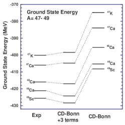
Figure 1: The experimental and theoretical ground state energy levels for A=47-49. The results in the second and third columns are labelled by their Hamiltonians.

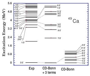
Figure 2: Experimental and theoretical excitation energy levels for ${}^{49}{Ca}$. Both CD-Bonn and CD-Bonn+3terms resultss are presented.

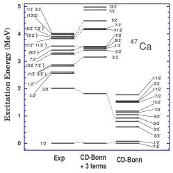
Figure 3: Experimental and theoretical excitation energy levels for ${}^{47}{Ca}$. Both CD-Bonn and CD-Bonn+3terms results are presented.

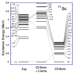
Figure 4: Experimental and theoretical excitation energy levels for ${}^{49}{Sc}$. Both CD-Bonn and CD-Bonn+3terms results are presented.

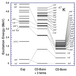
Figure 5: Experimental and theoretical excitation energy levels for ${}^{47}{K}$. Both CD-Bonn and CD-Bonn+3terms results are presented.

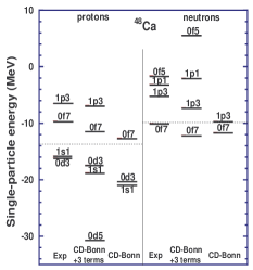
Figure 6: Experimental and theoretical levels that are dominantly single-proton and single-neutron particles or holes of ${}^{48}{Ca}$. The levels are labeled by (n, l, 2j), and the dashed lines are the Fermi energies.

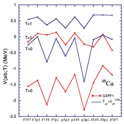
Figure 7: (color online) Comparison between CD-Bonn and GXPF1 of the monopole matrix elements V(ab;T)(A=48), which are shown by circles and squares, respectively. Lines are drawn to guide the eyes. The orbit pair label ”f7p3” stands for $a=f_{7/2}$ and $b=p_{3/2}$, for example.

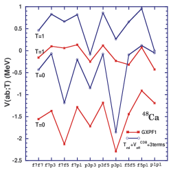
Figure 8: (color online)Comparison between CD-Bonn+3terms and GXPF1 of the monopole matrix elements V(ab;T)(A=48), which are shown by circles and squares, respectively. See the caption to Fig. 7.

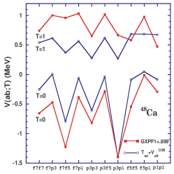
Figure 9: (color online) Comparison of the monopole matrix elements V(ab;T)(A=48) between CD-Bonn and GXPF1 (shifted to have an overall average monopole the same as CD-Bonn), which are shown by circles and squares, respectively. See the caption to Fig. 7.

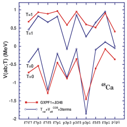
Figure 10: (color online) Comparison of the monopole matrix elements V(ab;T)(A=48) between CD-Bonn+3terms and GXPF1 (shifted to have an overall average monopole the same as CD-Bonn + 3 terms), which are shown by circles and squares, respectively. See the caption to Fig. 7.

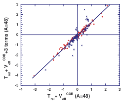
Figure 11: (color online) Correlation of V(abcd; JT) (A=48) matrix elements between CD-Bonn+3terms and CD-Bonn. The matrix elements of T=0 and T=1 are shown by open circles and crosses, respectively. There are no monopole shifts. The straight line represents a linear fit to all the matrix elements.

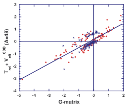
Figure 12: (color online) Correlation of V(abcd; JT)(A=48) between CD-Bonn and G. See the caption to Fig. 11.

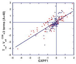
Figure 13: (color online) Correlation of the matrix elements V(abcd; JT)(A=48) between CD-Bonn+3terms and GXPF1. See the caption to Fig. 11.

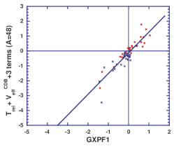
Figure 14: (color online) Correlation of the matrix elements V(abcd; JT)(A=48) between CD-Bonn+3terms and GXPF1, where we retain only the off-diagonal matrix elements, i.e. the 56 matrix elements that cannot contribute to a single-particle Hamiltonian (see text). See the caption to Fig. 11.

III.2 Excitation energy spectra

The excitation energy spectra for ${}^{49}Ca$, ${}^{47}Ca$, ${}^{49}Sc$ and ${}^{47}K$ are shown in Figs. 2-5 respectively. In every case the $\it{ab-initio}$ NCSM results with CD-Bonn are far too compressed relative to experiment - a feature also seen in the $A=48$ results [VPSN06] . Here, we trace this primary defect to the inferred properties of the neutron orbits. That is, the incorrect ground state spin seen in Fig. 2 and the absence of a significant excitation energy gap in Fig. 3 indicate the spin-orbit splitting of the neutrons is insufficient to provide proper subshell closure at the neutron $0f_{7/2}$ orbit. This defect is rectified in the results with CD-Bonn + 3 terms as seen by the corresponding spectra in Figs. 2 and 3. Similar tendencies have been seen before with valence G-matrix interactions and identified as a problem with the $L^{2}$ dependence of the single-particle states [MZPC96] ; [Caurier05] .

The CD-Bonn results in Figs. 4 and 5 are more difficult to interpret due to the glaring deficiencies just mentioned for the neutrons with the CD-Bonn Hamiltonian. We will show below that the proton shell closure is better established with CD-Bonn. This supports the assertion that the main deficiencies seen in the third columns of Figs. 4 and 5 are indeed likely to reside with the inferred neutron spin-orbit splitting problem.

The modified Hamiltonian provides greatly improved spectra for all four nuclei as seen in the second columns of Figs. 2-5. It is to be noted that these nuclei were not involved in the fitting procedure used to determine the parameters of the added phenomenological terms. Perhaps the most significant remaining deficiency is the incorrect ground state spin for ${}^{47}K$ as seen in Fig. 5. This is the first case of a nucleus in the region of $A=47$ to $A=49$ (12 nuclei studied to date) where we did not obtain the correct ground state spin with CD-Bonn + 3 terms Hamiltonian.

III.3 Single-particle characteristics

In order to better understand the underlying physics of our NCSM results, we investigated the single-particle-like properties of our solutions.

In a simple closed-shell nucleus, we expect the leading configuration of the ground state solution in our m-scheme treatment to be a single Slater determinant. Single-particle (or hole) excitations should be easily identified by the character of their leading configurations - i.e. a single-particle creation (or destruction) operator acting on the ground state Slater determinant of the reference nucleus ${}^{48}Ca$. For our odd-mass nuclei, this is the character we seek. That is, we take the standard phenomenological shell model configuration of a single Slater determinant with a closed sd-shell for the protons and a closed $f_{7/2}$ subshell for the neutrons and look for the appropriate states which have a single nucleon added to (or subtracted from) that Slater determinant. We accept states as ”single-particle-like” when we find one with a leading configuration having more than 50% probability to be in the simple configuration just described. When the majority weight is distributed over a few states, we use the centroid and we discuss those cases in some detail below. We were not successful in locating all the expected single-particle-like and single-hole-like states. That is, those absent from our presentation below were spread among a large number of eigenstates.

For a closed-shell nucleus (Z,N) the single-particle energies (SPE) for states above the Fermi surface are related to the binding energy differences:

$e_{p}^{>}=BE(Z,N)-BE^{*}(Z+1,N)$,
and

$e_{n}^{>}=BE(Z,N)-BE^{*}(Z,N+1)$.

The SPE for sates below the Fermi surface are given by

$e_{p}^{<}=BE^{*}(Z-1,N)-BE(Z,N),$
and

$e_{n}^{<}=BE^{*}(Z,N-1)-BE(Z,N)$.

The BE are ground state binding energies which are taken as positive values, and e will be negative for bound states. $(BE^{*}=BE-E_{x})$ is the ground state binding energy minus the excitation energy of the excited states associated with the single-particle states.

Experimental SPE’s and the results of our analysis are shown in Fig. 6. The experimental SPE’s for protons and neutrons follow B.A.Brown’s analysis [BAB01] . To guide the eye, we draw a horizontal line to indicate the vicinity of the Fermi surfaces for the protons and neutrons.

Fig. 6 shows that proton shell closure is established with both Hamiltonians, the CD-Bonn and the CD-Bonn+3 terms. The correct energy locations are better approximated with the modified Hamiltonian. Fig. 6 also shows that neutron subshell closure only appears with modified Hamiltonian. Here, the ordering is correct but the states are considerably more spread out compared with experiment.

Let us consider some of the details underlying the single-particle-like states. The situation for the $1p_{3/2}$ or ”$1p3$” state in the left panel of Fig. 6, the proton single-particle state in ${}^{49}Sc$, with the modified Hamiltonian, is quite interesting. It appears that this state is mixed over several excited states in the spectrum. We can take the strength spread over several states and construct a centroid for this $1p3$ state by a weighted average over the states carrying that strength. Here are the relevant input ingredients.

The first excited state of ${}^{49}Sc$ is a ${3/2}^{-}$, as seen in the second column of Fig. 4, with about 51% of the occupancy of the $1p3$ state. Its eigenvalue is -425.151 MeV compared to a ground state of -428.365 MeV. The 18th state in the ${}^{49}Sc$ spectrum is also a ${3/2}^{-}$ with 28% of the occupancy of the $1p3$ state. Its eigenvalue is -422.803MeV. The 24th state is also a ${3/2}^{-}$ with 21% of the occupancy of the $1p3$ state. Its eigenvalue is -422.440MeV.

Thus, to a good approximation, the $1p3$ strength is spread over these three states. We will identify the weighted average $[0.51\times(-428.365)+0.28\times(-422.803)+0.21\times(-422.440)]=-423.79$ as the centroid of the single particle $1p3$ state which we then include accordingly in the second column of the figure.

For the proton hole states with the modified Hamiltonian, we perform a detailed search up to excitation energies of about 14 MeV in the ${}^{47}K$ spectra. It appears that the $0d_{5/2}$ single-hole state is spread among many states with the largest observed concentration on the ${5/2}^{+}$ state at -386.17MeV (13.36 MeV of excitation energy). Here, we find a single $J^{\pi}={5/2}^{+}$ state in ${}^{47}K$ with 30 % $0d_{5/2}$ vacancy and we assign this state to our $0d_{5/2}$ single-hole state. Most of the $0d_{5/2}$ strength, however, was not observed among the limited number of converged eigenstates.

Let us consider the ${}^{49}Ca$ results with the modified Hamiltonian in the upper right panel of Fig. 6. The ground state is approximately a pure $[(1p_{3/2})^{1}(0f_{7/2})^{8}]$ configuration. We note that the spacing for the subshell closure is in good agreement with experiment while there is a shift of a couple MeV towards more binding in the model as previously indicated in Fig. 1. A nearly pure $1p_{1/2}$ single-particle state is obtained at 5.235 MeV excitation energy and an extra low-lying ${7/2}^{-}$ appears with 2p-1h character (see Fig. 2). Our lowest-lying ${5/2}^{-}$ consists of 2p-1h character relative to subshell closure.

We contrast the modified Hamiltonian’s results for the ${}^{49}Ca$ ground state with those obtained using the $\it{ab-initio}$ CD-Bonn where $[(1p_{3/2})^{4}(1p_{1/2})^{2}(0f_{7/2})^{3}]_{1/2^{-}}$ is the dominant configuration reflecting again the inadequacies of the neutron single-particle properties.

III.4 Monopole matrix elements V(ab;T)

The monopole matrix element is defined by an angular momentum average of coupled doubly-reduced two-body matrix elements:

$$V(ab;T)=\frac{\sum_{J}(2J+1)V(abab:JT)}{\sum_{J}(2J+1)}\;.$$ (6)

For our NCSM Hamiltonians the ”$V$” appearing in Eqn. 6 signifies the full 2-body intrinsic-coordinate Hamiltonian, $T_{rel}+V_{eff}$, except that we omit the Coulomb interaction from this analysis.

We examine the monopole character of our initial CD-Bonn Hamiltonian and we note some similarities and differences from the GXPF1 interaction[HOB04] as shown in Fig. 7. The see-saw shapes of the two Hamiltonians in Fig. 7 are similar but our Hamiltonian is shifted towards less attraction. Given the many differences between the respective theoretical starting points, the $\it{ab-initio}H_{eff}$ for the NCSM and the G-matrix for GXPF1 the different bare NN interactions, etc., the similarities observed in Fig. 7 are remarkable. In order to summarize a comparison of the underlying theoretical interactions, we list in Table 1a simplified overview of their differences and similarities.

For a more detailed comparison of the interactions, we present the fp-shell matrix elements applicable to the present investigation in Tables 2 and 3. For convenience in finding the major differences, we present two columns of key differences in the matrix elements: ”diff1” represents the difference between our $ab-initio~{}H_{eff}$ and our modified $H_{eff}$; and, ”diff2” represents the difference between our modified $H_{eff}$ and the GXPF1 interaction. While diff1 shows magnitudes that only occasionally exceed 1 MeV, diff2 shows magnitudes approaching 2.6 MeV. This type of comparison suggests that our solution for the modified Hamiltonian remains closer to our initial $H_{eff}$ derived from CD-Bonn, than it is to the fitted Hamiltonian, GXPF1.

Fig. 8 presents a similar comparison of the monopole character in the fp-shell of the two phenomenological Hamiltonians, GXPF1 and CD-Bonn + 3 terms. Overall, the changes in the monopole character due to the addition of the phenomenological terms to our $H_{eff}$ of Fig. 7 appear somewhat larger for the T=1 monopole than for T=0. The effect of ”+3 terms” is to increase the T=0 and T=1 splitting of six of the monopoles while the 4 remaining T=0 and T=1 monopole splittings are reduced.

In order to better visualize the similarities of the fp-shell matrix elements, we present in Figs. 9 and 10 the same comparisons shown in Figs. 7 and 8, respectively, with an overall shift of the GXPF1 monopole matrix elements so that the average over all monopole matrix elements is the same for the two Hamiltonians. Specifically the average shift of T=0 and T=1 monopoles for GXPF1 in Fig. 9 is 0.899768 MeV, while for GXPF1 in Fig. 10 it is 0.83485 MeV. It is now evident that both the CD-Bonn and CD-Bonn + 3 terms have monopoles with less $T=0$ and $T=1$ splittings.

III.5 Matrix element correlations

We present in Figs. 11-14 the correlations between pairs of fp-shell interaction matrix element sets. With Fig. 11, we observe the high degree of correlation between the 195 matrix elements of our starting Hamiltonian, CD-Bonn, and our modified Hamiltonian, CD-Bonn + 3 terms. This indicates that, for the most part, our Hamiltonian is minimally modified by the addition of the phenomenological terms. Such a high correlation is reminiscent of the high correlations seen between GXPF1 and its starting interaction, the G-matrix [HOB04] .

It is then very interesting to observe in Fig. 12 the lack of correlation between our starting Hamiltonian, CD-Bonn, and the G-matrix underlying the GXPF1 interaction. This lack of correlation reflects the major differences in the underlying theories that are summarized in Table 1.

Furthermore, we find minimal correlation between CD-Bonn + 3 terms and the full GXPF1 as seen in Fig. 13. This indicates the likely sensitivity to the starting Hamiltonians in the fitting procedures and to the differences in the NCSM compared to a valence shell model approach.

Finally, in order to isolate the true off-diagonal 2-body interaction effects from those that may lead to contributions to the single-particle energies, we eliminate some of the matrix elements from the comparison. In Fig. 14 we present the correlation of matrix elements V(abcd; JT)(A=48) between CD-Bonn+3terms and GXPF1, where we retain only those that cannot contribute to a single-particle Hamiltonian in leading order. That is, we eliminate all two-body matrix elements where at least one single-particle-state (sps) of the bra equals a sps of the ket. There are 56 remaining two-body matrix elements. Clearly, the correlation improves. This suggests that those eliminated matrix elements would generate single-particle properties, in leading order, different from the single-particle properties embodied in GXPF1 plus its associated single-particle energies. Comparisons of spectra and other properties with these Hamiltonians as one proceeds further from A=48 could shed more light on their differences.

IV Conclusions and outlook

We have presented an initial NCSM investigation of the spectral properties of the $A=47$ and $A=49$ nuclei that are one nucleon away from doubly-magic ${}^{48}Ca$. We have shown that the NCSM with a previously introduced modified Hamiltonian produces spectral properties in reasonable accord with experiment. Shell closure properties are obtained and a path has been opened for multi-shell investigations of these nuclei within the NCSM. We are undertaking such additional investigations. Also, for a better understanding of various fp-shell interactions we made a comparison between our initial and modified fp-shell matrix elements in the harmonic oscillator basis with the GXPF1 interaction [HOB04] and we found notable differences. Our initial and modified NCSM $H_{eff}$ matrix elements in the fp-shell are strongly correlated. However, the same matrix elements of the modified NCSM Hamiltonian appear to lack a significant correlation with the GXPF1 matrix elements (see Fig. 13). We found evidence (Fig. 14) suggesting that significant differences in single-particle properties may underly some of the distinctions between our $H_{eff}$ and the GXPF1 interaction. Additional applications could reveal those distinctions in greater detail.

V Acknowledgements

This work was partly performed under the auspices of the U. S. Department of Energy by the University of California, Lawrence Livermore National Laboratory under contract No. W-7405-Eng-48. This work was also supported in part by USDOE grant DE-FG-02 87ER40371, Division of Nuclear Physics, and in part by NSF grant INT0070789.

Hamiltonian Property	G-matrix	NCSM cluster $H_{eff}$
Oscillator parameter dependence	Yes	Yes
Depends on the choice of P-space	Yes	Yes
Translationally invariant	No	Yes
Reguires perturbative corrections
and raises known convergence issues	Yes	No
Starting energy dependence	Yes	No
Single-particle spectra dependence	Yes	No
A-dependence	No	Yes

Table 1: Overview of the differences and similarities of the two theoretical approaches that underlie the Hamiltonians whose matrix elements are compared in this work.

$2j_{a}$	$2j_{b}$	$2j_{c}$	$2j_{d}$	J	T	G	GXPF1	diff1	CD-Bonn	CD-Bonn	diff2
										+3 terms
7	3	7	3	5	0	-2.1167	-2.8504	-0.7337	-1.0390	-1.3413	-0.3023
3	3	5	5	0	1	-0.5243	-1.1968	-0.6725	-0.6019	-1.1129	-0.5109
7	7	7	7	3	0	-0.2309	-0.8087	-0.5778	0.5597	0.5555	-0.0042
7	5	7	5	6	0	-2.3465	-2.9159	-0.5693	-1.3743	-1.8599	-0.4856
7	5	7	5	5	0	-0.0203	-0.5845	-0.5642	0.5813	0.4117	-0.1693
3	1	3	1	2	1	-0.7965	-0.2822	0.5143	-0.0068	-0.4932	-0.4864
7	7	5	5	0	1	-1.9095	-1.3288	0.5806	-2.2586	-3.4709	-1.2123

Table 2: Comparison of selected two-body matrix elements V(abcd; JT) (Mev) (A=48) for which the difference between our interaction is large. Diff1 represents the difference between GXPF1 and G and diff2 is the difference between CD-Bonn+3terms and CD-Bonn.

							CD-Bonn
$2j_{a}$	$2j_{b}$	$2j_{c}$	$2j_{d}$	J	T	CD-Bonn	+3 terms	GXPF1	diff1	diff2
7	7	7	7	1	0	0.3073	-0.1114	-1.2334	0.4187	1.1219
7	7	7	7	3	0	0.5597	0.5555	-0.8087	0.0042	1.3642
7	7	7	7	5	0	0.2624	0.2831	-0.7531	-0.0207	1.0363
7	7	7	7	7	0	-1.1278	-1.4916	-2.5614	0.3638	1.0698
7	7	7	3	3	0	-0.3941	-0.5040	-0.8461	0.1099	0.3421
7	7	7	3	5	0	-0.7265	-0.9507	-0.4098	0.2242	-0.5409
7	7	7	5	1	0	2.1173	2.8631	1.8252	-0.7457	1.0379
7	7	7	5	3	0	0.9514	1.0655	1.0488	-0.1141	0.0167
7	7	7	5	5	0	0.7734	0.8348	1.2348	-0.0614	-0.4001
7	7	7	1	3	0	0.6495	0.8948	0.8534	-0.2453	0.0414
7	7	3	3	1	0	-0.2455	-0.3852	-0.4144	0.1398	0.0292
7	7	3	3	3	0	-0.3005	-0.4174	-0.3281	0.1169	-0.0894
7	7	3	5	1	0	-0.0853	-0.1703	-0.0871	0.0850	-0.0832
7	7	3	5	3	0	0.1932	0.2031	0.0722	-0.0099	0.1308
7	7	3	1	1	0	0.4140	0.5911	0.3026	-0.1771	0.2885
7	7	5	5	1	0	1.7698	1.7798	0.6255	-0.0100	1.1542
7	7	5	5	3	0	0.5251	0.3335	0.4187	0.1917	-0.0852
7	7	5	5	5	0	0.0925	-0.1388	0.1190	0.2313	-0.2578
7	7	5	1	3	0	0.0405	-0.0388	-0.1040	0.0792	0.0652
7	7	1	1	1	0	0.1906	0.1891	0.0260	0.0015	0.1630
7	3	7	3	2	0	0.5237	0.4452	-0.5179	0.0784	0.9632
7	3	7	3	3	0	0.1963	0.1499	-0.9660	0.0464	1.1159
7	3	7	3	4	0	0.8313	1.0290	-0.3550	-0.1978	1.3840
7	3	7	3	5	0	-1.0390	-1.3413	-2.8505	0.3022	1.5092
7	3	7	5	2	0	-0.8737	-1.2298	-0.6130	0.3561	-0.6168
7	3	7	5	3	0	0.3768	0.4786	0.2440	-0.1018	0.2346
7	3	7	5	4	0	-0.1160	-0.1168	0.1874	0.0008	-0.3042
7	3	7	5	5	0	0.4572	0.6186	0.6478	-0.1614	-0.0292
7	3	7	1	3	0	1.1174	1.3527	1.6188	-0.2353	-0.2661
7	3	7	1	4	0	0.0174	-0.1382	0.1639	0.1556	-0.3021
7	3	3	3	3	0	-0.3760	-0.4208	-0.4140	0.0447	-0.0068
7	3	3	5	2	0	-1.2556	-1.4158	-1.2209	0.1602	-0.1949
7	3	3	5	3	0	0.3921	0.3582	0.5563	0.0339	-0.1981
7	3	3	5	4	0	-0.6204	-0.5575	-0.6824	-0.0629	0.1249
7	3	3	1	2	0	-0.3442	-0.3473	-0.5983	0.0032	0.2510
7	3	5	5	3	0	0.3158	0.3418	0.1595	-0.0260	0.1823
7	3	5	5	5	0	0.0470	0.0157	0.0321	0.0312	-0.0164
7	3	5	1	2	0	1.1771	1.0398	1.0504	0.1372	-0.0105
7	3	5	1	3	0	0.4204	0.2798	0.6943	0.1407	-0.4146
7	5	7	5	1	0	-3.0683	-4.0586	-4.4003	0.9903	0.3417
7	5	7	5	2	0	-1.6830	-2.1268	-3.1243	0.4438	0.9975
7	5	7	5	3	0	-0.2221	-0.3923	-1.3469	0.1702	0.9545
7	5	7	5	4	0	-0.8282	-1.3239	-2.1696	0.4958	0.8457
7	5	7	5	5	0	0.5813	0.4117	-0.5845	0.1696	0.9962
7	5	7	5	6	0	-1.3743	-1.8599	-2.9159	0.4856	1.0560
7	5	7	1	3	0	-0.4566	-0.5755	-0.4085	0.1189	-0.1670
7	5	7	1	4	0	-0.7299	-0.9642	-0.3640	0.2343	-0.6002

							CD-Bonn
$2j_{a}$	$2j_{b}$	$2j_{c}$	$2j_{d}$	J	T	CD-Bonn	+3 terms	GXPF1	diff1	diff2
7	5	3	3	1	0	1.0540	1.4541	0.8564	-0.4000	0.5977
7	5	3	3	3	0	0.6228	0.9335	0.6018	-0.3108	0.3317
7	5	3	5	1	0	-0.9454	-0.9914	-1.2221	0.0461	0.2307
7	5	3	5	2	0	-0.9098	-1.3983	-0.5745	0.4885	-0.8238
7	5	3	5	3	0	-0.5037	-0.7272	-0.7413	0.2235	0.0141
7	5	3	5	4	0	-0.7302	-0.9373	-0.6156	0.2071	-0.3217
7	5	3	1	1	0	-1.6911	-2.4985	-1.4076	0.8074	-1.0909
7	5	3	1	2	0	-0.8349	-1.0867	-0.7142	0.2518	-0.3725
7	5	5	5	1	0	-0.7288	-1.3474	-0.2628	0.6186	-1.0846
7	5	5	5	3	0	0.5634	0.5072	0.6128	0.0562	-0.1056
7	5	5	5	5	0	0.9161	1.1081	1.0858	-0.1920	0.0223
7	5	5	1	2	0	0.6576	0.8630	0.5233	-0.2054	0.3397
7	5	5	1	3	0	0.5616	0.7463	0.6016	-0.1846	0.1447
7	5	1	1	1	0	0.0834	0.2459	0.1852	-0.1624	0.0606
7	1	7	1	3	0	-0.4452	-0.6265	-1.6302	0.1813	1.0037
7	1	7	1	4	0	0.2353	0.1281	-1.0186	0.1072	1.1467
7	1	3	3	3	0	0.4449	0.5872	0.6159	-0.1422	-0.0288
7	1	3	5	3	0	-0.3159	-0.5871	-0.0340	0.2712	-0.5531
7	1	3	5	4	0	-1.2649	-1.4129	-1.3073	0.1480	-0.1056
7	1	5	5	3	0	-0.2768	-0.4766	-0.2518	0.1998	-0.2248
7	1	5	1	3	0	0.2871	0.3689	0.4328	-0.0818	-0.0639
3	3	3	3	1	0	0.0709	-0.3114	-0.6060	0.3822	0.2947
3	3	3	3	3	0	-0.9009	-1.0857	-2.1991	0.1848	1.1134
3	3	3	5	1	0	-0.1096	-0.1431	0.2280	0.0335	-0.3711
3	3	3	5	3	0	0.1404	0.0837	0.2187	0.0567	-0.1350
3	3	3	1	1	0	1.7185	2.1121	1.7350	-0.3936	0.3771
3	3	5	5	1	0	0.1123	0.1144	0.0464	-0.0021	0.0680
3	3	5	5	3	0	-0.1931	-0.3294	-0.0525	0.1363	-0.2769
3	3	5	1	3	0	0.0218	0.0295	0.1105	-0.0077	-0.0810
3	3	1	1	1	0	0.8627	0.9239	0.7374	-0.0613	0.1866
3	5	3	5	1	0	-1.1592	-1.2747	-2.6191	0.1156	1.3444
3	5	3	5	2	0	-0.2345	-0.2183	-1.4517	-0.0161	1.2333
3	5	3	5	3	0	0.3962	0.5057	-0.5629	-0.1095	1.0686
3	5	3	5	4	0	0.1063	-0.0482	-1.0455	0.1545	0.9973
3	5	3	1	1	0	-0.3476	-0.3027	-0.9540	-0.0450	0.6513
3	5	3	1	2	0	-0.3270	-0.3718	-0.4693	0.0448	0.0976
3	5	5	5	1	0	0.3981	0.5114	0.4583	-0.1134	0.0532
3	5	5	5	3	0	0.3474	0.5234	0.3074	-0.1760	0.2160

							CD-Bonn
$2j_{a}$	$2j_{b}$	$2j_{c}$	$2j_{d}$	J	T	CD-Bonn	+3 terms	GXPF1	diff1	diff2
3	5	5	1	2	0	0.4842	0.7654	0.3401	-0.2812	0.4253
3	5	5	1	3	0	0.8234	0.9535	0.9752	-0.1302	-0.0217
3	5	1	1	1	0	0.5210	0.5287	0.7817	-0.0078	-0.2530
3	1	3	1	1	0	-1.4397	-1.9339	-2.4084	0.4942	0.4744
3	1	3	1	2	0	-1.3841	-1.8107	-2.2214	0.4266	0.4107
3	1	5	5	1	0	0.1552	0.1834	-0.0324	-0.0282	0.2158
3	1	5	1	2	0	0.2759	0.2561	0.6629	0.0197	-0.4068
3	1	1	1	1	0	0.4259	0.2031	0.8157	0.2228	-0.6126
5	5	5	5	1	0	0.5809	0.5578	-0.8215	0.0231	1.3793
5	5	5	5	3	0	0.5560	0.7603	-0.5379	-0.2042	1.2982
5	5	5	5	5	0	-0.6845	-0.8166	-2.1920	0.1321	1.3754
5	5	5	1	3	0	-0.4343	-0.5141	-0.6030	0.0798	0.0889
5	5	1	1	1	0	-0.1464	-0.2172	-0.3037	0.0708	0.0864
5	1	5	1	2	0	0.6529	0.8651	-0.3049	-0.2122	1.1700
5	1	5	1	3	0	-0.3858	-0.4207	-1.3472	0.0349	0.9265
1	1	1	1	1	0	-0.0865	-0.0553	-1.1943	-0.0312	1.1390
7	7	7	7	0	1	-0.3350	-2.0599	-2.3427	1.7249	0.2829
7	7	7	7	2	1	0.1443	-0.0627	-0.8985	0.2070	0.8358
7	7	7	7	4	1	0.5554	0.5520	-0.1245	0.0035	0.6765
7	7	7	7	6	1	0.7456	0.7885	0.2674	-0.0429	0.5211
7	7	7	3	2	1	-0.3418	-0.6840	-0.4957	0.3422	-0.1883
7	7	7	3	4	1	-0.1909	-0.3059	-0.2852	0.1150	-0.0207
7	7	7	5	2	1	-0.0952	-0.2651	0.2082	0.1699	-0.4733
7	7	7	5	4	1	-0.3340	-0.6119	-0.4803	0.2779	-0.1316
7	7	7	5	6	1	-0.5566	-0.8969	-0.5421	0.3402	-0.3547
7	7	7	1	4	1	-0.2668	-0.3767	-0.2014	0.1099	-0.1753
7	7	3	3	0	1	-0.5835	-1.2136	-0.6892	0.6301	-0.5244
7	7	3	3	2	1	-0.2066	-0.3701	-0.1942	0.1635	-0.1759
7	7	3	5	2	1	-0.2271	-0.2046	-0.1657	-0.0225	-0.0389
7	7	3	5	4	1	-0.2018	-0.3594	-0.2137	0.1575	-0.1457
7	7	3	1	2	1	-0.1860	-0.3622	-0.0353	0.1761	-0.3269
7	7	5	5	0	1	-2.2587	-3.4709	-1.3289	1.2123	-2.1420
7	7	5	5	2	1	-0.4434	-1.0308	-0.1958	0.5874	-0.8350
7	7	5	5	4	1	-0.2330	-0.5665	-0.0318	0.3335	-0.5347
7	7	5	1	2	1	-0.3465	-0.5240	-0.1244	0.1776	-0.3996
7	7	1	1	0	1	-0.5140	-0.9231	-0.3651	0.4091	-0.5580
7	3	7	3	2	1	0.1202	-0.3894	-0.5842	0.5096	0.1948
7	3	7	3	3	1	0.6896	0.9356	0.1500	-0.2460	0.7857

							CD-Bonn
$2j_{a}$	$2j_{b}$	$2j_{c}$	$2j_{d}$	J	T	CD-Bonn	+3 terms	GXPF1	diff1	diff2
7	3	7	3	4	1	0.6401	0.6043	-0.1343	0.0357	0.7387
7	3	7	3	5	1	0.7681	1.4989	0.5686	-0.7307	0.9303
7	3	7	5	2	1	-0.0119	-0.1848	0.0921	0.1730	-0.2769
7	3	7	5	3	1	-0.0815	-0.3396	-0.5025	0.2581	0.1629
7	3	7	5	4	1	-0.1517	-0.2794	-0.2388	0.1277	-0.0405
7	3	7	5	5	1	0.0043	-0.5487	-0.4621	0.5531	-0.0866
7	3	7	1	3	1	0.0600	-0.1725	-0.1007	0.2325	-0.0718
7	3	7	1	4	1	-0.3353	-0.6527	-0.3219	0.3173	-0.3307
7	3	3	3	2	1	-0.2402	-0.3588	-0.3591	0.1185	0.0004
7	3	3	5	2	1	-0.4330	-0.5878	-0.5223	0.1548	-0.0655
7	3	3	5	3	1	0.0012	0.1176	0.1764	-0.1164	-0.0587
7	3	3	5	4	1	-0.5820	-0.8194	-0.4367	0.2374	-0.3827
7	3	3	1	2	1	-0.2734	-0.3242	-0.4095	0.0508	0.0852
7	3	5	5	2	1	-0.5131	-0.6285	0.0845	0.1154	-0.7131
7	3	5	5	4	1	-0.1958	-0.2548	-0.2062	0.0590	-0.0486
7	3	5	1	2	1	-0.8563	-1.3191	-0.7715	0.4628	-0.5476
7	3	5	1	3	1	-0.0252	-0.0957	-0.1743	0.0705	0.0786
7	5	7	5	1	1	0.5082	2.4886	-0.0854	-1.9804	2.5740
7	5	7	5	2	1	0.7226	0.6164	-0.1681	0.1062	0.7845
7	5	7	5	3	1	0.6587	1.8189	0.6055	-1.1602	1.2134
7	5	7	5	4	1	0.6129	0.4423	0.4576	0.1706	-0.0153
7	5	7	5	5	1	0.6787	1.6340	0.7141	-0.9554	0.9199
7	5	7	5	6	1	-0.3906	-1.0421	-0.9527	0.6515	-0.0895
7	5	7	1	3	1	-0.0360	0.6988	0.3097	-0.7349	0.3891
7	5	7	1	4	1	-0.0990	-0.2726	0.1832	0.1736	-0.4558
7	5	3	3	2	1	-0.0618	0.0096	0.0689	-0.0715	-0.0593
7	5	3	5	1	1	-0.1021	0.5367	0.0501	-0.6388	0.4866
7	5	3	5	2	1	-0.1821	-0.3153	-0.4080	0.1332	0.0927
7	5	3	5	3	1	-0.0857	-0.1165	-0.0257	0.0308	-0.0907
7	5	3	5	4	1	-0.4104	-0.5206	-0.2593	0.1101	-0.2613
7	5	3	1	1	1	-0.0507	-0.4156	0.0530	0.3649	-0.4686
7	5	3	1	2	1	-0.1190	-0.3124	-0.0147	0.1934	-0.2977
7	5	5	5	2	1	-0.4658	-0.6595	-0.4825	0.1936	-0.1770
7	5	5	5	4	1	-0.3706	-0.5363	-0.2603	0.1657	-0.2760
7	5	5	1	2	1	-0.3356	-0.3388	-0.1477	0.0032	-0.1911
7	5	5	1	3	1	0.0577	-0.2258	0.1062	0.2835	-0.3320
7	1	7	1	3	1	0.7343	1.4734	0.4682	-0.7391	1.0052
7	1	7	1	4	1	0.4269	0.3100	-0.1294	0.1169	0.4394

							CD-Bonn
$2j_{a}$	$2j_{b}$	$2j_{c}$	$2j_{d}$	J	T	CD-Bonn	+3 terms	GXPF1	diff1	diff2
7	1	3	5	3	1	0.0358	0.3366	0.3738	-0.3009	-0.0372
7	1	3	5	4	1	-0.6006	-0.9045	-0.5871	0.3039	-0.3174
7	1	5	5	4	1	-0.2879	-0.3606	-0.2160	0.0727	-0.1446
7	1	5	1	3	1	-0.0740	-0.0480	-0.1524	-0.0260	0.1044
3	3	3	3	0	1	-0.2470	-1.4569	-1.0727	1.2099	-0.3842
3	3	3	3	2	1	0.3792	0.1916	-0.0852	0.1875	0.2768
3	3	3	5	2	1	-0.0594	-0.0203	-0.4449	-0.0390	0.4246
3	3	3	1	2	1	-0.5458	-0.9685	-0.6091	0.4227	-0.3594
3	3	5	5	0	1	-0.6019	-1.1128	-1.1968	0.5109	0.0839
3	3	5	5	2	1	-0.0825	-0.2487	0.0691	0.1662	-0.3177
3	3	5	1	2	1	-0.1325	-0.1434	-0.1847	0.0109	0.0414
3	3	1	1	0	1	-1.2996	-2.0501	-1.4342	0.7506	-0.6160
3	5	3	5	1	1	0.6068	1.5042	0.3155	-0.8974	1.1887
3	5	3	5	2	1	0.8432	0.8865	0.3466	-0.0432	0.5398
3	5	3	5	3	1	0.7102	1.4885	0.3324	-0.7783	1.1561
3	5	3	5	4	1	0.4260	0.1411	-0.2483	0.2848	0.3894
3	5	3	1	1	1	-0.0955	0.5019	-0.1034	-0.5975	0.6053
3	5	3	1	2	1	-0.1390	-0.2215	-0.4367	0.0825	0.2151
3	5	5	5	2	1	-0.0040	-0.2060	-0.0538	0.2021	-0.1522
3	5	5	5	4	1	-0.0532	-0.2108	-0.3473	0.1576	0.1365
3	5	5	1	2	1	-0.2637	-0.5793	-0.3884	0.3156	-0.1909
3	5	5	1	3	1	-0.0287	0.4308	0.0576	-0.4595	0.3732
3	1	3	1	1	1	0.7211	1.5211	-0.1531	-0.8000	1.6742
3	1	3	1	2	1	-0.0068	-0.4932	-0.2823	0.4864	-0.2109
3	1	5	5	2	1	-0.2235	-0.3536	0.0576	0.1301	-0.4112
3	1	5	1	2	1	-0.2449	-0.3398	-0.2392	0.0950	-0.1006
5	5	5	5	0	1	0.3171	-1.0579	-1.1607	1.3749	0.1028
5	5	5	5	2	1	0.5129	0.5285	-0.4440	-0.0156	0.9724
5	5	5	5	4	1	0.8190	0.9119	-0.1560	-0.0929	1.0679
5	5	5	1	2	1	-0.1027	-0.3641	-0.3082	0.2614	-0.0559
5	5	1	1	0	1	-0.3086	-0.7120	-0.7775	0.4034	0.0656
5	1	5	1	2	1	0.5515	0.3998	-0.1459	0.1517	0.5457
5	1	5	1	3	1	0.7763	1.3514	0.2289	-0.5751	1.1224
1	1	1	1	0	1	0.6719	-0.0072	-0.4294	0.6791	0.4222

Table 3: Comparison of the fp-shell two-body matrix elements V(abcd; JT) (Mev) (A=48) employed in this work. The interaction GXPF1 is taken from Ref. [HOB04] . Diff1 represents the difference between CD-Bonn+3terms and CD-Bonn and Diff2 is the difference between CD-Bonn+3terms and GXPF1.

References

- (1) T.W. Burrows, Nucl. Data Sheets, 74, 1 (1995); Nucl. Data Sheets 76, 191 (1995).
- (2) Electronic version of Nucl. Data Sheets, telnet://bnlnd2.dne.bnl.gov
- (3) G. Martinez-Pinedo, A.P. Zuker, A. Poves and E. Caurier, nucl-th/9608044.
- (4) B. A. Brown, Progr. Part. Nucl. Phys. 47, 517 (2001).
- (5) T. Otsuka, M. Honma, T. Mizusaki, N. Shimizu, and Y. Utsuno, Prog. Part. Nucl. Phys. 47, 319 (2001).
- (6) D.J. Dean, T. Engeland, M. Hjorth-Jensen, M. Kartamychev and E. Osnes, Prog. Part. Nucl. Phys. 53 419(2004).
- (7) E. Caurier, G. Martinez-Pinedo, F. Nowacki, A. Poves and A. P. Zuker, Rev. Mod. Phys. 77 427(2005).
- (8) A. Poves, E. Pasquini and A.P. Zuker, Phys. Lett. B82, 319 (1979); A. Poves and A.P. Zuker, Phys. Rep. 70, 235 (1981).
- (9) J.P. Vary, S. Popescu, S. Stoica and P. Navrátil, nucl-th/0607041.
- (10) J.P. Vary, ”Many-Fermion Dynamics Code,” (1992, unpublished); J.P. Vary and D.C Zheng, ibid, (1994,unpublished).
- (11) R. Machleidt, F. Sammarruca and Y. Song, Phys. Rev. C 53, 1483 (1996); R. Machleidt, Phys. Rev. C 63, 024001 (2001).
- (12) M. Honma, T. Otsuka, B. A. Brown and T. Mizusaki, Phys. Rev. C 65, 061301(r) (2002); Phys. Rev. C 69, 034335 (2004).
- (13) K.D. Sviratcheva, J.P. Draayer and J.Vary, Phys. Rev. C 73, 034324 (2006).
- (14) D. C. Zheng, B. R. Barrett, L. Jaqua, J. P. Vary, and R. L. McCarthy, Phys. Rev. C 48, 1083 (1993); D. C. Zheng, J. P. Vary, and B. R. Barrett, Phys. Rev. C 50, 2841 (1994); D. C. Zheng, B. R. Barrett, J. P. Vary, W. C. Haxton, and C. L. Song, Phys. Rev. C 52, 2488 (1995).
- (15) P. Navrátil and B. R. Barrett, Phys. Rev. C 54, 2986 (1996); Phys. Rev. C 57, 3119 (1998).
- (16) P. Navrátil and B. R. Barrett, Phys. Rev. C 57, 562 (1998).
- (17) P. Navrátil and B. R. Barrett, Phys. Rev. C 59, 1906 (1999); P. Navrátil, G. P. Kamuntavičius and B. R. Barrett, Phys. Rev. C 61, 044001 (2000).
- (18) P. Navrátil, J. P. Vary and B. R. Barrett, Phys. Rev. Lett. 84, 5728 (2000); Phys. Rev. C 62, 054311 (2000).
- (19) P. Navrátil, J. P. Vary, W. E. Ormand and B. R. Barrett, Phys. Rev. Lett. 87, 172502 (2001). E. Caurier, P. Navrátil, W. E. Ormand and J. P. Vary, Phys. Rev. C 64, 051301 (2001).
- (20) S. Okubo, Prog. Theor. Phys. 12, 603 (1954); J. Da Providencia and C. M. Shakin, Ann. of Phys. 30, 95 (1964); S.Y. Lee and K. Suzuki, Phys. Lett. 91B, 79 (1980); K. Suzuki and S.Y. Lee, Prog. of Theor. Phys. 64, 2091 (1980); K. Suzuki, Prog. Theor. Phys. 68, 246 (1982); K. Suzuki, Prog. Theor. Phys. 68, 1999 (1982); K. Suzuki and R. Okamoto, Prog. Theor. Phys. 70, 439 (1983).
- (21) R. B. Wiringa, V. G. J. Stoks, and R. Schiavilla, Phys. Rev. C 51, 38 (1995).
- (22) C.P. Viazminsky and J.P. Vary, J. Math. Phys., 42, 2055 (2001).
- (23) H. Kamada, et. al, Phys. Rev. C 64 044001(2001).
- (24) I. Stetcu, B.R. Barrett, P. Navrátil and J. P. Vary, Phys. Rev. C 71, 044325(2005); I. Stetcu, B.R. Barrett, P. Navrátil and C.W. Johnson, Int. J. Mod. Phys. E 14, 95 (2005); I. Stetcu, B.R. Barrett, P. Navrátil and J. P. Vary, Phys. Rev. C 73, 037307(2006).
- (25) A. Nogga, P. Navrátil, B.R. Barrett and J.P. Vary, Phys. Rev. C 73, 064002 (2006), and references therein.
- (26) M.A. Hasan, J.P. Vary, and P. Navrátil, Phys. Rev. C 69, 034332 (2004) .
- (27) O. Atramentov, J.P. Vary and P. Navrátil, in preparation.
- (28) A. C. Hayes, P. Navrátil and J. P. Vary, Phys. Rev. Lett. 91, 012502 (2003).
- (29) A.M. Shirokov, A.I. Mazur, S.A. Zaytsev, J.P. Vary and T.A. Weber, Phys. Rev. C 70, 044005 (2004).
- (30) A. M. Shirokov, J. P. Vary, A. I. Mazur, S. A. Zaytsev and T. A. Weber, Phys. Letts. B 621, 96 (2005).
- (31) A.M. Shirokov, J.P. Vary, A.I. Mazur and T.A. Weber, nucl-th/0512105.
- (32) J. P. Vary, D. Chakrabarti, A. Harindranath, R. Lloyd, L. Martinovic and J. R. Spence, Coherent States and Spontaneous Symmetry Breaking in Light Front Scalar Field Theory , Proceedings of the Workshop On Light-Cone QCD And Nonperturbative Hadron Physics 2005 (LC 2005), 7-15 July 2005, Cairns, Queensland, Australia, and references therein.