Electromagnetic nucleon form factors in instant and point form

Abstract

We present a study of the electromagnetic structure of the nucleons with constituent quark models in the framework of relativistic quantum mechanics. In particular, we address the construction of spectator-model currents in the instant and point forms. Corresponding results for the elastic nucleon electromagnetic form factors as well as charge radii and magnetic moments are presented. We also compare results obtained by different realistic nucleon wave functions stemming from alternative constituent quark models. Finally, we discuss the theoretical uncertainties that reside in the construction of spectator-model transition operators.

I Introduction

A promising approach to the nucleon electromagnetic (EM) structure at low and moderate momentum transfers consists in employing constituent quark models (CQMs) in the framework of relativistic quantum mechanics (RQM). Different forms of RQM, such as the instant, front, and point forms, have been used by various authors (e.g., in Refs. Cardarelli:1995dc ; Szczepaniak:1995mi ; Merten:2002nz ; Pace:2003aa ; Julia-Diaz:2003gq ). Realistic descriptions of the EM nucleon form factors were specifically obtained with the Goldstone-boson-exchange (GBE) CQM. Working within the point form, the electric and magnetic form factors of both the proton and the neutron were described in surprisingly good agreement with experimental data Wagenbrunn:2000es ; Boffi:2001zb . Similarly, the electric radii and magnetic moments of all the octet and decuplet baryon ground states were reproduced as well Berger:2004yi . By an analogous calculation also the axial nucleon form factors could be explained consistently Glozman:2001zc . Until now, it remains as a puzzle why the direct quark-model predictions in point form fall so close to experiment in all aspects of the electroweak nucleon structure, especially since simplified spectator-model current operators have been employed and no additional parametrizations have been introduced. It is noteworthy that the point-form results are also very similar to the parameter-free predictions of the instanton-induced (II) CQM of the Bonn group that were calculated in a completely different approach along the Bethe-Salpeter formalism Merten:2002nz . The quality of the reproduction of the baryon EM properties gave impulse to studies of strong decays of baryon resonances along the same formalisms. However, the corresponding decay widths are not described equally well Melde:2005hy ; Melde:2004qu ; Sengl:2006gz ; Melde:2006yw ; Sengl:2007yq ; Metsch:2003ix .

In order to clarify the situation we undertook a closer inspection of the point-form spectator model (PFSM) in Ref. Melde:2004qu . We demonstrated along the strong decay widths that some significant effects may be caused by ambiguities connected to the fact that a unique spectator-model construction cannot be obtained by imposing Poincaré invariance alone. It was already observed before that further constraints should be included Polyzou:1986df ; Lev:1995ann . This property is inherent to any form of RQM and in this paper we specifically discuss the effects of such ambiguities in the instant form spectator model (IFSM) and the PFSM.

We address the proton and neutron electromagnetic form factors at momentum transfers up to $Q^{2}=4$ GeV². First we introduce the construction of instant-form and point-form spectator-model currents and characterize their particular properties. We then derive their nonrelativistic limits and show that both, IFSM and PFSM, lead to the same result, namely, the well-known nonrelativistic impulse approximation (NRIA). We provide a comparison of the IFSM, PFSM and NRIA predictions of the GBE CQM Glozman:1998ag . Subsequently, we examine the effects from different realistic CQMs relying on distinct quark-quark dynamics. In particular, we discuss the PFSM results by the GBE CQM in relation to the ones of a one-gluon-exchange (OGE) CQM, namely the relativistic version of the Bhaduri-Cohler-Nogami (BCN) CQM Bhaduri:1981pn as parametrized in Ref. Theussl:2000sj . In this context a comparison is made also with the form-factor results reported from the II CQM by the Bonn group Merten:2002nz . Finally, in line with Refs. Polyzou:1986df ; Lev:1995ann , we discuss how additional constraints like charge normalization and time-reversal invariance can be exploited to reduce as much as possible some remaining ambiguities in the present form of the spectator-model constructions. We end the paper in Sect. IV with a summary and conclusion.

II Electromagnetic Current

In RQM the nucleon states are expressed as eigenstates $\left|P,J,\Sigma\right>$ of the interacting mass operator

$$\hat{M}=\hat{M}_{\rm free}+\hat{M}_{\rm int}\,,$$ (1)

the intrinsic spin operator $\hat{J}$, and its z-component $\hat{\Sigma}$ (the letters without hat denoting the corresponding eigenvalues). The covariant normalization of these states is

$$\left<P^{\prime},J^{\prime},\Sigma^{\prime}|P,J,\Sigma\right>=2P_{0}\delta^{3}\left({\vec{P}}-{\vec{P}}^{\prime}\right)\delta_{JJ^{\prime}}\delta_{\Sigma\Sigma^{\prime}}\,.$$ (2)

The mass operator $\hat{M}$ is connected to the four-momentum operator $\hat{P}$ and the four-velocity operator $\hat{V}$ by the relations

$$\hat{P}^{\mu}={\hat{M}}\hat{V}^{\mu}\,,$$ (3)

where

$$\hat{P}^{\mu}\hat{P}_{\mu}=\hat{M}^{2}\,.$$ (4)

Because of the commutation relations among these operators the nucleon eigenstates with mass $M$ can equivalently be denoted as $\left|V,M,J,\Sigma\right>$. In this notation the elastic transition amplitude between the incoming and outgoing nucleon eigenstates is given by the following matrix element of the reduced electromagnetic current operator

$$F^{\mu}_{\Sigma^{\prime},\Sigma}\left(Q^{2}\right)=\left<V^{\prime},M,\frac{1}{2},\Sigma^{\prime}\right|{\hat{J}}^{\mu}_{\rm rd}\left|V,M,\frac{1}{2},\Sigma\right>\,,$$ (5)

where $Q^{2}=(P^{\prime\mu}-P^{\mu})^{2}$ is the momentum transfer by the virtual photon. In the Breit frame, the nucleon electric and magnetic Sachs form factors, $G_{\rm E}\left(Q^{2}\right)$ and $G_{\rm M}\left(Q^{2}\right)$, are related to the transition amplitude $F^{\mu}_{\Sigma^{\prime},\Sigma}$ by

$$F^{0}_{\Sigma^{\prime},\Sigma}\left(Q^{2}\right) = 2MG_{\rm E}\left(Q^{2}\right)\delta_{\Sigma^{\prime}\Sigma}$$ (6)

$${\vec{F}}_{\Sigma^{\prime},\Sigma}\left(Q^{2}\right) = iQG_{\rm M}\left(Q^{2}\right)\chi^{\dagger}_{\Sigma^{\prime}}\left({\vec{\sigma}}\times{\vec{e}}_{z}\right)\chi_{\Sigma}^{\phantom{\dagger}}\,,$$ (7)

where $\Sigma^{\prime},\Sigma=\pm\frac{1}{2}$ are the projections of the nucleon spin $\vec{\sigma}$ along the direction ${\vec{e}}_{z}$ of the $z$-axis and $\chi$ are the corresponding Pauli spinors. The form factors also lead directly to the magnetic moments

$$\mu=G_{\rm M}\left(Q^{2}=0\right)$$ (8)

and the charge radii

$$r^{2}_{\rm ch}=\left.-6\frac{dG_{\rm E}}{d\left(Q^{2}\right)}\right|_{Q^{2}=0}\,.$$ (9)

The electric and magnetic form factors in Eqs. (6) and (7) are Poincaré invariant, since both the mass-operator eigenstates and the electromagnetic current operator transform under the Poincaré group. Depending on the particular form of RQM (instant, front, or point forms) certain generators of the Poincaré transformations become interaction dependent while the other ones belong to the kinematical subgroup.

It is still rather difficult to employ the full (many-body) structure of the current operator and thus one adheres to simplifications. The common form consists in the so-called spectator approximation. The definition of a spectator-model current operator is generally not unique and requires additional constraints. In particular, the spectator-model construction has to be covariant under the transformations of the kinematic subgroup of the particular form of RQM and it must guarantee for time-reversal invariance. Further it should reduce to a sum of genuine single-particle currents in the limit of vanishing interaction among the constituent quarks and yield the charge of the proton for the electric form factor approaching momentum transfer $Q^{2}=0$. In addition, the construction should lead to a proper nonrelativistic limit.

II.1 Instant-Form Spectator Model

In the instant form the spatial translations and rotations form the kinematic subgroup, whereas the boosts become interaction dependent.

In the explicit calculations of the matrix elements (5) one requires momentum eigenstates of the free three-quark system $\left|p_{1},p_{2},p_{3};\sigma_{1},\sigma_{2},\sigma_{3}\right>$ defined as tensor products of single-particle momentum eigenstates $\left|p_{i};\sigma_{i}\right>$. In any reference frame with total three-momentum $\vec{P}=\sum_{i}{\vec{p}_{i}}$ they can also be expressed as

$$\left|\vec{P};\vec{k}_{1},\vec{k}_{2},\vec{k}_{3};\mu_{1},\mu_{2},\mu_{3}\right>=\\ \sum_{\sigma_{i}}\prod_{i}{D_{\sigma_{i}\mu_{i}}^{\frac{1}{2}}\left\{R_{W}\left[k_{i};B\left(v\right)\right]\right\}}\left|p_{1},p_{2},p_{3};\sigma_{1},\sigma_{2},\sigma_{3}\right>\,,$$ (10)

wherein the Wigner rotations depend on the free four velocity

$$v=\frac{P_{\rm free}}{M_{\rm free}}=\frac{\sum_{i}{p_{i}}}{\sum_{i}{\omega_{i}}}\,.$$ (11)

The momenta $k_{i}$ are connected to the momenta $p_{i}$ by the Boost relations $p_{i}=B(v)k_{i}$ and they fulfill the constraint $\sum_{i}{\vec{k}_{i}}=0$. The individual quark energies are given by $\omega_{i}=\sqrt{m_{i}^{2}+\vec{k}_{i}^{2}}$. The $\mu_{i}$ correspond to the individual quark spins in the rest frame of the three-quark system. The free momentum eigenstates of Eq. (10) have the following completeness relation

$$\mathbf{1}=\sum_{\mu_{i}}{\int{d^{3}\vec{P}d^{3}\vec{k}_{2}d^{3}\vec{k}_{3}\frac{\sum_{i}{\omega_{i}}}{E_{\rm free}}\frac{1}{2\omega_{1}2\omega_{2}2\omega_{3}}}}\\ \times\left|\vec{P};\vec{k}_{1},\vec{k}_{2},\vec{k}_{3};\mu_{1},\mu_{2},\mu_{3}\right>\left<\vec{P};\vec{k}_{1},\vec{k}_{2},\vec{k}_{3};\mu_{1},\mu_{2},\mu_{3}\right|\,.$$ (12)

They are well suited for instant-form calculations because here the three-momentum $\vec{P}$ is not affected by interactions. Representing the nucleon states with this basis allows to separate the internal motion according to

$$\left<\vec{P}^{\prime};\vec{k}^{\prime}_{1},\vec{k}^{\prime}_{2},\vec{k}^{\prime}_{3};\mu^{\prime}_{1},\mu^{\prime}_{2},\mu^{\prime}_{3}|\vec{P},J,\Sigma\right>=\\ \sqrt{2E^{\prime}_{\rm free}E}\sqrt{\frac{2\omega^{\prime}_{1}2\omega^{\prime}_{2}2\omega^{\prime}_{3}}{\sum{\omega^{\prime}_{i}}}}\delta^{3}\left(\vec{P}^{\prime}-\vec{P}\right)\Psi_{M\frac{1}{2}\Sigma}\left({\vec{k}}_{i};\mu_{i}\right)\,,$$ (13)

where $E^{\prime}_{\rm free}$ and $E$ are the eigenvalues of the zeroth components of the free and interacting four-momenta $\hat{P}^{\prime\mu}_{\rm free}$ and $\hat{P}^{\mu}$, respectively. The wave function $\Psi_{M\frac{1}{2}\Sigma}\left({\vec{k}}_{i};\mu_{i}\right)$ is just the rest-frame wave function of the nucleon. It is normalized to unity

$$\sum_{\mu_{i}}\int{d^{3}k_{2}d^{3}k_{3}}\Psi^{\star}_{M\frac{1}{2}\Sigma^{\prime}}\left(\vec{k}_{i};\mu_{i}\right)\Psi_{M\frac{1}{2}\Sigma}\left(\vec{k}_{i};\mu_{i}\right)=\delta_{\Sigma\Sigma^{\prime}}$$ (14)

in accordance with the normalization condition of the nucleon eigenstates in Eq. (2).

The transition amplitude (5) in instant form can then be expressed as

$$F^{\mu}_{\Sigma^{\prime},\Sigma}\left(Q^{2}\right) = 2\sqrt{EE^{\prime}}\sum_{\sigma_{i}\sigma^{\prime}_{i}}\sum_{\mu_{i}\mu^{\prime}_{i}}{\int{d^{3}{\vec{k}}_{2}d^{3}{\vec{k}}_{3}d^{3}{\vec{k}}^{\prime}_{2}d^{3}{\vec{k}}^{\prime}_{3}}}\frac{1}{\sqrt{E_{\rm free}E^{\prime}_{\rm free}}}\sqrt{\frac{\sum{\omega_{i}}}{2\omega_{1}2\omega_{2}2\omega_{3}}}\sqrt{\frac{\sum{\omega^{\prime}_{i}}}{2\omega^{\prime}_{1}2\omega^{\prime}_{2}2\omega^{\prime}_{3}}}$$ (15)

$${\Psi^{\star}_{M\frac{1}{2}\Sigma^{\prime}}\left({\vec{k}}^{\prime}_{i};\mu^{\prime}_{i}\right)\prod_{\sigma^{\prime}_{i}}{D_{\sigma^{\prime}_{i}\mu^{\prime}_{i}}^{\star\frac{1}{2}}\left\{R_{W}\left[k^{\prime}_{i};B\left(v^{\prime}\right)\right]\right\}}}$$

$$\left<p^{\prime}_{1},p^{\prime}_{2},p^{\prime}_{3};\sigma^{\prime}_{1},\sigma^{\prime}_{2},\sigma^{\prime}_{3}\right|{\hat{J}}^{\mu}_{\rm rd}\left|p_{1},p_{2},p_{3};\sigma_{1},\sigma_{2},\sigma_{3}\right>\prod_{\sigma_{i}}{D_{\sigma_{i}\mu_{i}}^{\frac{1}{2}}\left\{R_{W}\left[k_{i};B\left(v\right)\right]\right\}}\Psi_{M\frac{1}{2}\Sigma}\left({\vec{k}}_{i};\mu_{i}\right)\,,$$

The spectator model of the current operator in instant form (the IFSM) is then defined as

$$\left<p^{\prime}_{1},p^{\prime}_{2},p^{\prime}_{3};\sigma^{\prime}_{1},\sigma^{\prime}_{2},\sigma^{\prime}_{3}\right|{\hat{J}}^{\mu}_{\rm rd,IFSM}\left|p_{1},p_{2},p_{3};\sigma_{1},\sigma_{2},\sigma_{3}\right>=\\ 3e_{1}{\bar{u}}\left(p^{\prime}_{1},\sigma^{\prime}_{1}\right)\gamma^{\mu}u\left(p_{1},\sigma_{1}\right)\\ 2p_{20}\delta^{3}\left({\vec{p}}_{2}-{\vec{p}}^{\prime}_{2}\right)2p_{30}\delta^{3}\left({\vec{p}}_{3}-{\vec{p}}^{\prime}_{3}\right)\delta_{\sigma_{2}\sigma^{\prime}_{2}}\delta_{\sigma_{3}\sigma^{\prime}_{3}}\,.$$ (16)

As a consequence of the very properties of the instant form (with the three-momenta as generators of spatial translations lying in the kinematic subgroup) the momenta of the struck quark in the incoming and outgoing nucleon are related by

$$p_{10}-p^{\prime}_{10} = \tilde{q}_{0}$$

$$\vec{p}_{1}-\vec{p}^{\prime}_{1} = \vec{Q}\,.$$ (17)

This means that the whole three-momentum carried by the virtual photon is transferred to the quark 1, while only a part of the photon energy is absorbed by a single quark, i.e. $\tilde{q}_{0}\neq Q_{0}$. Clearly, $\tilde{q}_{0}$ is uniquely determined by overall momentum conservation and the two spectator conditions. We shall see below that in the point form the spectator-model construction leads to a different relation between $p_{1}$ and $p^{\prime}_{1}$, as the momenta no longer lie in the kinematic subgroup.

The construction (16) is usually adopted in the Breit frame. When transformed to a different reference frame, it does not preserve its spectator-model structure but acquires additional many-body contributions. Thus, in general, the IFSM current should not be viewed as a one-body operator. Furthermore a spectator-model construction made in another reference frame defines a different spectator-model current. As a result the calculation done with an IFSM current defined in the Breit frame leads to a different result than the calculation performed with an IFSM current defined in the laboratory frame, say. In this sense the IFSM, while always yielding Poincaré invariant results, bears an ambiguity in the construction, as it is per se frame dependent. If one imposes time-reversal invariance on the IFSM, one necessarily has to resort to the Breit frame. In all other reference frames additional many-body contributions would be needed to guarantee for time-reversal invariance.

Eq. (15) exhibits all the effects of the Lorentz boosts on the incoming and outgoing nucleon states through the changes in the respective quark momenta and the Wigner $D$-functions. Sometimes the latter are simply ignored by setting them to unity Li:2007hn . While this simplifies the calculations considerably, the resulting form factors obtained in this way are no longer strictly Poincaré invariant.

II.2 Point-Form Spectator Model

In the point form the kinematic subgroup is the Lorentz group, only the space-time translations are interaction dependent. For the actual calculations it is advantageous to use velocity states (of the free three-quark system) defined by

$$\left|v;\vec{k}_{1},\vec{k}_{2},\vec{k}_{3};\mu_{1},\mu_{2},\mu_{3}\right>=\\ \sum_{\sigma_{i}}\prod_{i}{D_{\sigma_{i}\mu_{i}}^{\frac{1}{2}}\left\{R_{W}\left[k_{i};B\left(v\right)\right]\right\}}\left|p_{1},p_{2},p_{3};\sigma_{1},\sigma_{2},\sigma_{3}\right>\,,$$ (18)

where the momenta $k_{i}$ and $p_{i}$ are again connected through the boost relation $p_{i}=B\left(v\right)k_{i}$ and the $k_{i}$ satisfy $\sum_{i}{\vec{k}_{i}}=0$.

Since in the point form the four-velocity $v=(v_{0},\vec{v})$ is independent of the interaction, it can be expressed through eigenvalues of the free or interacting momentum and mass operators as

$$v=\frac{P_{\rm free}}{M_{\rm free}}=\frac{P}{M}=V\,.$$ (19)

The completeness relation for the velocity states reads

$${\mathbf{1}}=\sum_{\mu_{i}}\int{d^{3}{\vec{v}}d^{3}{\vec{k}}_{2}d^{3}{\vec{k}}_{3}\frac{\left(\sum_{i}{\omega_{i}}\right)^{3}}{v_{0}}\frac{1}{2\omega_{1}2\omega_{2}2\omega_{3}}}\\ \times\left|v;\vec{k}_{1},\vec{k}_{2},\vec{k}_{3};\mu_{1},\mu_{2},\mu_{3}\right\rangle\left\langle v;\vec{k}_{1},\vec{k}_{2},\vec{k}_{3};\mu_{1},\mu_{2},\mu_{3}\right|\,.$$ (20)

Representing the nucleon states in the velocity-state basis allows to separate the internal motion in the following way

$$\left\langle v;\vec{k}_{1},\vec{k}_{2},\vec{k}_{3};\mu_{1},\mu_{2},\mu_{3}|V,M,\frac{1}{2},\Sigma\right\rangle\\ =\frac{\sqrt{2}}{M}v_{0}\delta^{3}\left(\vec{v}-\vec{V}\right)\sqrt{\frac{2\omega_{1}2\omega_{2}2\omega_{3}}{\left(\sum_{i}{\omega_{i}}\right)^{3}}}\Psi_{M\frac{1}{2}\Sigma}\left(\vec{k}_{i};\mu_{i}\right)\,,$$ (21)

which differs substantially from the separation followed in the instant form, Eq. (13). However, the $\Psi_{M\frac{1}{2}\Sigma}\left(\vec{k}_{i};\mu_{i}\right)$ is again the rest-frame wave function of the nucleon. The nucleon mass eigenstates in Eq. (21) are normalized as in Eq. (2) and the wave functions are normalized as in Eq. (14).

The transition amplitude, Eq. (5), of the electromagnetic current in point form reads

$$F^{\mu}_{\Sigma^{\prime},\Sigma}\left(Q^{2}\right) = \frac{2}{M^{2}}\sum_{\sigma_{i}\sigma^{\prime}_{i}}\sum_{\mu_{i}\mu^{\prime}_{i}}{\int{d^{3}{\vec{k}}_{2}d^{3}{\vec{k}}_{3}d^{3}{\vec{k}}^{\prime}_{2}d^{3}{\vec{k}}^{\prime}_{3}}}\sqrt{\frac{\left(\omega_{1}+\omega_{2}+\omega_{3}\right)^{3}}{2\omega_{1}2\omega_{2}2\omega_{3}}}\sqrt{\frac{\left(\omega^{\prime}_{1}+\omega^{\prime}_{2}+\omega^{\prime}_{3}\right)^{3}}{2\omega^{\prime}_{1}2\omega^{\prime}_{2}2\omega^{\prime}_{3}}}$$ (22)

$${\Psi^{\star}_{M\frac{1}{2}\Sigma^{\prime}}\left({\vec{k}}^{\prime}_{i};\mu^{\prime}_{i}\right)\prod_{\sigma^{\prime}_{i}}{D_{\sigma^{\prime}_{i}\mu^{\prime}_{i}}^{\star\frac{1}{2}}\left\{R_{W}\left[k^{\prime}_{i};B\left(V^{\prime}\right)\right]\right\}}}$$

$$\left<p^{\prime}_{1},p^{\prime}_{2},p^{\prime}_{3};\sigma^{\prime}_{1},\sigma^{\prime}_{2},\sigma^{\prime}_{3}\right|{\hat{J}}^{\mu}_{\rm rd,PFSM}\left|p_{1},p_{2},p_{3};\sigma_{1},\sigma_{2},\sigma_{3}\right>\prod_{\sigma_{i}}{D_{\sigma_{i}\mu_{i}}^{\frac{1}{2}}\left\{R_{W}\left[k_{i};B\left(V\right)\right]\right\}}\Psi_{M\frac{1}{2}\Sigma}\left({\vec{k}}_{i};\mu_{i}\right)\,,$$

and the spectator-model approximation of the current operator in point form (the PFSM) is defined by the expression

$$\left<p^{\prime}_{1},p^{\prime}_{2},p^{\prime}_{3};\sigma^{\prime}_{1},\sigma^{\prime}_{2},\sigma^{\prime}_{3}\right|{\hat{J}}^{\mu}_{\rm rd,PFSM}\left|p_{1},p_{2},p_{3};\sigma_{1},\sigma_{2},\sigma_{3}\right>=\\ 3{\cal N}e_{1}{\bar{u}}\left(p^{\prime}_{1},\sigma^{\prime}_{1}\right)\gamma^{\mu}u\left(p_{1},\sigma_{1}\right)\\ 2p_{20}\delta^{3}\left({\vec{p}}_{2}-{\vec{p}}^{\prime}_{2}\right)2p_{30}\delta^{3}\left({\vec{p}}_{3}-{\vec{p}}^{\prime}_{3}\right)\delta_{\sigma_{2}\sigma^{\prime}_{2}}\delta_{\sigma_{3}\sigma^{\prime}_{3}}\,.$$ (23)

Here the momentum transfer to the struck quark is given by

$$p^{\mu}_{1}-{p^{\prime}}^{\mu}_{1}=\tilde{q}^{\mu}\,,$$ (24)

where $\tilde{q}^{\mu}\neq Q^{\mu}$ is uniquely determined by the overall momentum conservation and the two spectator conditions. The relation between $p_{1}$ and $p^{\prime}_{1}$ is complicated, because the transferred momentum $\tilde{q}$ to the active quark inherits nontrivial interaction-dependent contributions Melde:2004qu . The momentum transfers to the struck quark in IFSM, Eq. (II.1), and in PFSM, Eq. (24), are rather different, because in the instant form the kinematical subgroup includes the three-momentum, whereas in point form it does not. Contrary to the IFSM, the PFSM maintains its spectator-model character in all reference frames. Always, only one quark is directly coupled to the photon, and the PFSM current is manifestly covariant. In the limit of vanishing quark-quark interaction such differences disappear and one recovers $\tilde{q}^{\mu}\rightarrow Q^{\mu}$.

Formally, the above definition of Eq. (23) looks the same as for the IFSM in Eq. (16) except for the appearance of an extra factor $\cal N$. The factor $\cal N$ is needed in the point form in order to yield the proper proton charge from the electric form factor in the limit $Q^{2}\rightarrow 0$ and to recover a sum of individual-particle currents when the interaction is turned off Melde:2004qu . In the works Wagenbrunn:2000es ; Glozman:2001zc ; Boffi:2001zb ; Berger:2004yi a choice of $\cal N$ symmetric with regard to the incoming and outgoing nucleon states was adopted

$${\cal N}={\cal N}_{\rm S}=\left(\frac{M}{\sum_{i}{\omega_{i}}}\right)^{\frac{3}{2}}\left(\frac{M}{\sum_{i}{\omega^{\prime}_{i}}}\right)^{\frac{3}{2}}\,.$$ (25)

It is important to notice that the factor $\cal N$ has nothing to do with the normalization of the nucleon states: the nucleon states follow the covariant normalization as in Eq. (2) implying, together with the normalization of the wave function in Eq. (14), the factors explicitly written out in Eq. (22); the factor ${\cal N}$ must be considered as part of the definition of the PFSM current and it is required to produce a consistent spectator-model operator in the point form.

One should note that both $\cal N$ and $\tilde{q}$ effectively depend on all three quark variables, and therefore the PFSM must not be considered strictly as a one-body operator. It effectively includes many-body contributions Melde:2004qu . The factor $\cal N$ can in principle be adopted in several ways. Later on we shall come back to this issue.

II.3 Nonrelativistic Impulse Approximation

The nonrelativistic reduction of both the IFSM and the PFSM leads to the same result, namely, to the nonrelativistic impulse approximation (NRIA):

$$F^{\mu\rm NR}_{\Sigma^{\prime},\Sigma}\left(Q^{2}\right) = \left<V^{\prime},M,\frac{1}{2},\Sigma^{\prime}\right|{\hat{J}}^{\mu}_{\rm rd,NR}\left|V,M,\frac{1}{2},\Sigma\right>=2M\sum_{\mu_{i}\mu^{\prime}_{i}}\int{d^{3}{\vec{k}}_{2}d^{3}{\vec{k}}_{3}d^{3}{\vec{k}}^{\prime}_{2}d^{3}{\vec{k}}^{\prime}_{3}}$$ (26)

$$\Psi^{\star}_{M\frac{1}{2}\Sigma^{\prime}}\left({\vec{k}}^{\prime}_{i};\mu^{\prime}_{i}\right){j}^{\mu}_{\rm rd,NR}\left(Q^{2}\right)\Psi_{M\frac{1}{2}\Sigma}\left({\vec{k}}_{i};\mu_{i}\right)$$

with

$${j}^{\mu}_{\rm rd,NR}\left(Q^{2}\right)=\\ e_{1}\begin{pmatrix}1\\ \\ \left[\frac{\vec{p}_{1}+\vec{p}^{\prime}_{1}}{2m_{1}}+\frac{i\vec{\sigma}_{1}\times\left(\vec{p}_{1}-\vec{p}^{\prime}_{1}\right)}{2m_{1}}\right]\delta^{3}\left(\vec{p}_{2}-\vec{p}^{\prime}_{2}\right)\delta^{3}\left(\vec{p}_{3}-\vec{p}^{\prime}_{3}\right)\end{pmatrix}$$ (27)

and the momenta now being connected through the relations $\vec{k}_{i}=\vec{p}_{i}-\frac{m_{i}}{\sum_{i}{m_{i}}}\vec{P}$ and $\vec{p}_{1}-\vec{p}^{\prime}_{1}=\vec{Q}$.

As is evident, all integration measures, normalization factors, and Wigner rotations have reduced to unity and the nonrelativistic expression for the EM current is recovered.

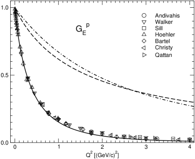
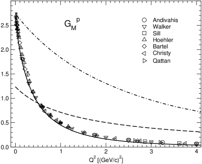
Figure 1: Electric and magnetic form factors of the proton as predicted by the GBE CQM with the the IFSM (dashed line), PFSM (full line), and the NRIA (dash-dotted line) current operators. Experimental data are from Refs. Lung:1993bu ; Markowitz:1993hx ; Rock:1982gf ; Bruins:1995ns ; Gao:1994ud ; Anklin:1994ae ; Anklin:1998ae ; Xu:2000xw ; Kubon:2001rj ; Xu:2002xc and Andivahis:1994rq ; Walker:1989af ; Sill:1993qw ; Hohler:1976ax ; Bartel:1973rf ; Christy:2004rc ; Qattan:2004ht .

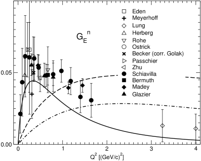
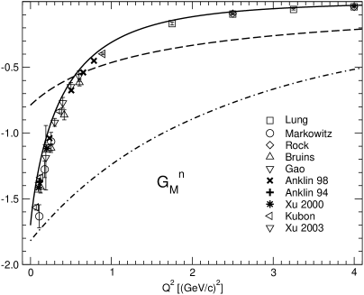
Figure 2: Same as in Fig. 1 but for the neutron. Experimental data are from Refs. Lung:1993bu ; Markowitz:1993hx ; Rock:1982gf ; Bruins:1995ns ; Gao:1994ud ; Anklin:1994ae ; Anklin:1998ae ; Xu:2000xw ; Kubon:2001rj ; Xu:2002xc ; Eden:1994ji ; Meyerhoff:1994ev ; Herberg:1999ud ; Rohe:1999sh ; Ostrick:1999xa ; Becker:1999tw ; Passchier:1999cj ; Zhu:2001md ; Schiavilla:2001qe ; Bermuth:2003qh ; Madey:2003av ; Glazier:2004ny .

III Elastic Nucleon Form Factors

In this section we present the theoretical results for the elastic electromagnetic form factors of the nucleon calculated with the spectator-model currents constructed above. First we compare the IFSM and PFSM results along the GBE CQM. Then we show the influences from different quark-model wave functions by comparing the GBE CQM results with the predictions of the BCN-OGE CQM. We stress that these results have been obtained without any parameter variation. However, there reside ambiguities in spectator-model constructions, which are discussed here quantitatively in case of the PFSM.

III.1 IFSM versus PFSM results

Figs. 1 and 2 contain the direct predictions for the Sachs form factors obtained from the GBE CQM. Tables 1 and 2 give the corresponding magnetic moments and charge radii. Immediately some striking features are evident. For the electric form factors of both proton and neutron the IFSM results are very similar to the NRIA and especially in case of the proton, they lie far off the experimental data. The PFSM predictions fall close to experiment Boffi:2001zb . For the magnetic form factors the IFSM and NRIA results become quite distinct, especially for lower momentum transfers. This has the consequence that the IFSM magnetic moments for both proton and neutron turn out to be unreasonable in comparison with experiment, while the NRIA results happen to reproduce them quite well (see Table 1).

Evidently, the spectator-model approximations are different in the instant and point forms even though they have the same nonrelativistic limit. The relativistic effects stem from the Lorentz boosts. In PFSM Lorentz boosts belong to the kinematic subgroup while in IFSM they do not. Consequently the two forms introduce different effective many-body contributions in the spectator operators. Therefore, we may interpret the differences between the IFSM and PFSM results as being due to different contributions from (effective) many-body contributions.

Table 1: Magnetic moments of the proton and neutron (in n.m.) as predicted by the GBE CQM with the the IFSM, PFSM, and the NRIA current operators. Experimental data after the PDG PDBook .

	GBE CQM			Experiment
Nucleon	IFSM	PFSM	NRIA
p	1.24	2.70	2.74	2.79
n	-0.79	-1.70	-1.82	-1.91

Table 2: Charge radii of the proton and neutron (in fm²) as predicted by the GBE CQM with the the IFSM, PFSM, and the NRIA current operators. Experimental data after the PDG PDBook .

	GBE CQM			Experiment
Nucleon	IFSM	PFSM	NRIA
p	0.156	0.824	0.102	0.766
n	-0.020	-0.135	-0.009	-0.116

It should be emphasized that we make the comparison of the IFSM, PFSM, and NRIA predictions without any readjustment of the CQM parameters. Here, we directly employ the nucleon wave function as produced by the GBE CQM, whose parameters were fitted only to the baryon spectra in Ref. Glozman:1998ag . One could bring, for example, the IFSM results closer to experiment by an ad-hoc modification of the nucleon wave function and an adjustment of the constituent quark mass, as is done in Ref. Julia-Diaz:2003gq . However, this would then change also the PFSM and NRIA results considerably, making a consistent comparison of the CQM predictions obtained with the various spectator-model constructions difficult if not impossible.

III.2 Effects from Quark-Model Wave Functions

Having compared the results with different spectator-model constructions of the EM current (in case of the GBE CQM), we are now interested to see the effects from different relativistic CQM nucleon wave functions. This comparison is performed along the PFSM approach. In addition to the GBE CQM (whose hyperfine interaction is flavour dependent) we have calculated the predictions of a different relativistic CQM with a chromomagnetic hyperfine interaction based on OGE dynamics. In particular, we have employed the relativistic variant of the BCN CQM Bhaduri:1981pn in the parametrization of Ref. Theussl:2000sj . For completeness we have also included the predictions by even another type of relativistic CQM, namely the II CQM by the Bonn group Loring:2001kx ; Loring:2001ky . These results, however, stem from the field-theoretic Bethe-Salpeter approach which is principally different from the RQM we followed. The current operator employed in Ref. Merten:2002nz has also been approximated by a spectator-model construction.

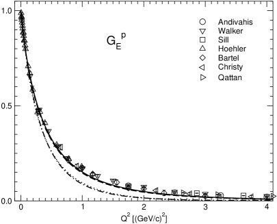
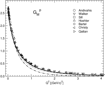
Figure 3: Electric and magnetic form factors of the proton as predicted by the GBE (full line) and BCN (dashed line) CQMs along the PFSM approach; in addition the results for the case with only the confinement potential (inherent in the GBE CQM) are given (dash-dotted line). For comparison also the predictions of the II CQM (dotted line) after Ref. Merten:2002nz are shown. Experimental data as in Fig. 1.

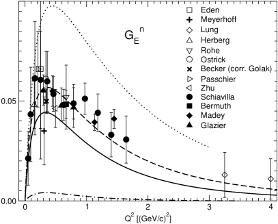
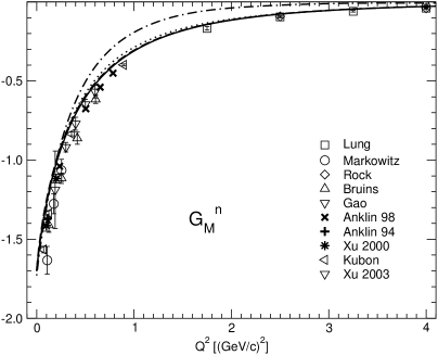
Figure 4: Same as in Fig. 3 but for the neutron. Experimental data as in Fig. 2.

In Figs 3 and 4 we compare the predictions for the EM form factors of proton and neutron, respectively; the corresponding results for the electric radii and magnetic moments are quoted in Tables 3 and 4. One observes that the differences between the GBE and BCN CQMs are relatively small; in most cases the curves are even indistinguishable. Only for the electric form factor of the neutron the discrepancies between the curves are clearly visible, but here one should take into account the expanded scale in that figure. Differences between the GBE and BCN CQMs are also found in the charge radii, whereas the magnetic moments are again very similar. In all instances, the PFSM predictions of the GBE and OGE CQMs are, nevertheless, found in remarkable vicinity of the experimental data, except for the electric radius of the neutron in case of the BCN CQM. Certainly, the differences between the two types of CQMs are much smaller than the variations found above between the IFSM and PFSM results.

It is now interesting to compare also with the predictions of the II CQM. Surprisingly, they are very similar to the ones of the GBE and OGE CQMs, even though they have been derived in a completely different framework, namely along the Bethe-Salpeter approach. Only, the results from the II CQM tend to undershoot the proton electric form factor and overestimate the neutron electric form factor but generally there is a similarity of the Bethe-Salpeter and PFSM results.

On the other hand, a CQM, where only the confinement potential is present, fails in reproducing the electromagnetic nucleon structure. In particular, it yields the proton form factors too small and misses the neutron electric form factor completely. The reason is that a certain mixed-symmetric spatial component in the neutron wave function is needed in order to produce a non-vanishing electric form factor. However, the neutron wave function produced by the confinement-only potential comes practically without a mixed-symmetric spatial part. That such type of nucleon wave function cannot be adequate is consistent with observations made already in earlier works sprung ; chernyak .

Table 3: Magnetic moments of the proton and neutron (in n.m.) as predicted by the GBE, BCN and confinement-only (CONF) CQMs along the PFSM and the II CQM along the Bethe-Salpeter (BS) approach. Experimental data after the PDG PDBook .

	PFSM			BS	Experiment
Nucleon	GBE	BCN	CONF	II
p	2.70	2.74	2.65	2.74	2.79
n	-1.70	-1.70	-1.73	-1.70	-1.91

Table 4: Charge radii of the proton and neutron (in fm²) as predicted by the GBE, BCN and confinement-only (CONF) CQMs along the PFSM and the II CQM along the Bethe-Salpeter (BS) approach. Experimental data after the PDG PDBook .

	PFSM			BS	Experiment
Nucleon	GBE	BCN	CONF	II
p	0.824	1.029	0.766	0.67	0.766
n	-0.135	-0.263	-0.009	-0.11	-0.116

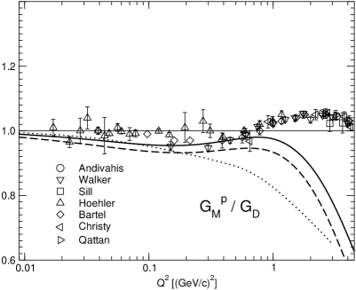
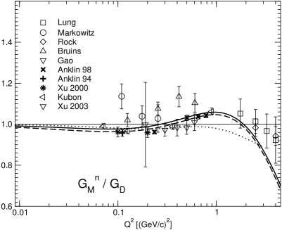
Figure 5: Same comparison as in Figs. 3 and 4 for the ratios of magnetic to dipole form factors of the proton (left panel) and the neutron (right panel). All ratios are normalized to $1$ at $Q^{2}=0$.

For a closer inspection of the differences in the relativistic CQM predictions it is instructive to look through the magnifying glass of $G_{M}^{n}/G_{D}$ and $G_{M}^{p}/G_{D}$ ratios. This comparison is given in Fig. 5. The tiny differences between the PFSM predictions of the GBE and OGE CQMs are confirmed. The $Q^{2}$ dependence of the ratios is seen to be slightly distinct in the case of the II CQM.

From the comparisons made in this subsection we conclude that realistic nucleon wave functions are necessary in order to describe the proton as well as neutron electromagnetic structure consistently. Such type of wave functions are obviously achieved in the GBE, OGE, and II CQMs. With respect to the nucleon electromagnetic structure the presence of a hyperfine interaction itself is found of considerable importance. Even though the various hyperfine interactions of the CQMs considered here stem from different dynamics, they obviously lead to similar nucleon wave functions. When the hyperfine interaction is left out completely (cf. the case with the confinement potential only), the nucleon structure can by no means be described in a reasonable manner.

III.3 Uncertainties in the PFSM Construction

Finally we deal with the problem that the PFSM construction has some residual ambiguity. In particular, a factor ${\cal N}$ necessarily appears in the PFSM current of Eq. (23). As already mentioned the factor ${\cal N}$ is unavoidable, if one wants the spectator model current to reduce to a genuine one-body operator in the limit of zero-momentum transfer Melde:2004qu . It is also required to guarantee for the proper charge normalization of the proton.

All results for the electromagnetic nucleon structure considered so far have been calculated with the symmetric choice for the factor ${\cal N}$ as given in Eq. (25). However, this is not the only possibility. Following Ref. Melde:2004qu one could also adopt the general expression

$${\cal N}\left(x,y\right)=\left(\frac{M}{\sum_{i}{\omega_{i}}}\right)^{xy}\left(\frac{M}{\sum_{i}{\omega^{\prime}_{i}}}\right)^{x\left(1-y\right)}\,,$$ (28)

where $x$ and $y$ are to be considered as open parameters varying in the range $0\leq x$ and $0\leq y\leq 1$. The normalization factors so defined are all Lorentz invariant and all lead to a covariant PFSM current with the required properties.

In the following, we examine the dependence of the EM form factor results on possible choices of $\cal N$, i.e. variations of the parameters $x$ and $y$. At zero momentum transfer the factor $\cal N$ depends only on $x$. In Fig. 6 we show the results for the electric proton form factor $G_{\rm E}^{p}\left(Q^{2}\right)$ at $Q^{2}=0$, i.e. the proton charge, for varying $x$. Clearly, the only possibility consistent with the proton charge normalization is $x=3$. This result is in line also with the arguments given in Ref. Melde:2004qu that in the limit $Q^{2}\rightarrow 0$ the PFSM reduces to a genuine one-body operator only with a cubic choice for the factor ${\cal N}$.

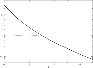
Figure 6: Electric proton form factor $G_{E}^{p}$ at momentum transfer $Q^{2}=0$ (i.e. proton charge) as a function of the exponent parameter $x$ in the PFSM factor $\cal N$ of Eq. (28), calculated with the GBE CQM Glozman:1998ag .

Once the parameter $x$ is uniquely fixed, let us now examine the possible $y$-dependence. In Fig. 7 we show the third component of the transition amplitude (22) in the Breit frame as a function of $y$ for three different momentum transfers. It is well known that in the Breit frame the expectation value of the third component of the current has to vanish under the constraint of time-reversal invariance Durand:1962 ; Ernst:1960 . From the results in Fig. 7 it is immediately seen that there is a unique value of $y$ where the third component of the transition amplitude vanishes for all values of $Q^{2}$. Consequently, $y=\frac{1}{2}$ has to be chosen in Eq. (28) in order to satisfy time-reversal invariance. This motivates the symmetric choice in Eq. (25).

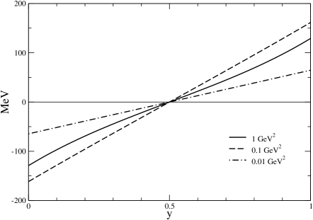
Figure 7: Third component of the transition amplitude $F^{3}_{\frac{1}{2},\frac{1}{2}}\left(Q^{2}\right)$ in the Breit frame as a function of the exponent parameter $y$ in the PFSM factor $\cal N$ of Eq. (28) for three different values of the momentum transfer $Q^{2}$, calculated with the GBE CQM Glozman:1998ag .

However, we may even find another choice for the factor $\cal N$ that meets all requirements posed, including time-reversal invariance. A valid construction would also be

$${\cal N}\left(z\right)=\frac{1}{2}\left[\left(\frac{M}{\sum_{i}{\omega_{i}}}\right)^{3z}\left(\frac{M}{\sum_{i}{\omega^{\prime}_{i}}}\right)^{3\left(1-z\right)}+\left(\frac{M}{\sum_{i}{\omega_{i}}}\right)^{3\left(1-z\right)}\left(\frac{M}{\sum_{i}{\omega^{\prime}_{i}}}\right)^{3z}\right]\,.$$ (29)

with an open parameter $z$ varying in the range $0\leq z\leq 1$. This expression produces the symmetric choice of Eq. (25) for the special value $z=\frac{1}{2}$.

Another form is obtained by choosing $z=0$ (or equivalently $z=1$), leading to

$${\cal N}_{\rm ari}=\frac{1}{2}\left[\left(\frac{M}{\sum_{i}{\omega_{i}}}\right)^{3}+\left(\frac{M}{\sum_{i}{\omega^{\prime}_{i}}}\right)^{3}\right]\,,$$ (30)

which can be viewed as the arithmetic mean of two pieces relating to the ratios of the interacting and free masses in the incoming and outgoing nucleon states.

Evidently, all of the allowed forms of $\cal N$, according to Eqs. (28) and (29), lead to the same nonrelativistic limit, which consists in the NRIA.

In summary we note that under the given premises there remains a certain ambiguity in the PFSM construction related to the factor $\cal N$. Let us thus examine the variations in the predictions for EM form factors resulting from different possible choices of $\cal N$. In Fig. 8 we show the ratios of neutron and proton magnetic form factors to the standard dipole form factors as obtained in the PFSM with three particular choices of $\cal N$; the solid line is the ${\cal N}_{S}$ result and the dashed line represents the results with ${\cal N}_{\rm ari}$. Fig. 9 contains the same comparisons for the proton electric to magnetic as well as electric to dipole form factor ratios. The band of variations in the predictions is limited by the cases with ${\cal N}_{\rm ari}$ and ${\cal N}_{\rm S}$. The uncertainty bands are anyway rather narrow since one must take into account that these ratios are extremely sensitive to small differences. For comparison we have added in Figs. 8 and 9 also the results obtained in IFSM (dashed-double-dotted lines).

Different choices of ${\cal N}\left(z\right)$ in Eq. (29) imply distinct $Q^{2}$-dependences in the form factors. One may ask which particular value of $z$ is favoured by phenomenology. We have thus performed a simple one-parameter fit of ${\cal N}\left(z\right)$ to the experimental data of the ratios $G_{M}^{n}/G_{D}$ and $G_{M}^{p}/G_{D}$ at a single intermediate momentum transfer of $Q^{2}=3$ GeV². It leads to $z=\frac{1}{6}$ and produces the results represented by the dash-dotted lines in Fig. 8. They lie everywhere in between the upper and lower bounds obtained with ${\cal N}_{\rm ari}$ and ${\cal N}_{\rm S}$, respectively.

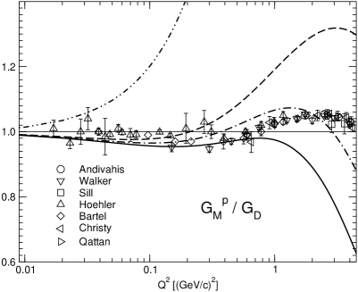
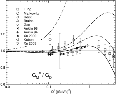
Figure 8: Ratios of magnetic form factor to standard dipole paramterization for the proton (left) and neutron (right) with different PFSM currents in case of the GBE CQM. The full lines denote the results with ${\cal N}_{\rm S}$ from the previous subsections, the dashed lines with ${\cal N}_{\rm ari}$ from Eq. (30), and the dash-dotted lines with ${\cal N}_{\rm fit}$, see the text. For comparison also the IFSM results are shown (dash-double-dotted lines). All ratios are normalized to $1$ at $Q^{2}=0$.

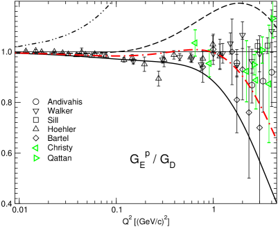
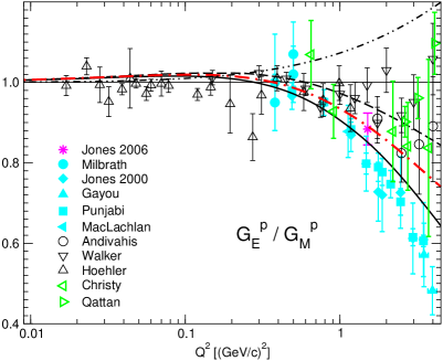
Figure 9: Same comparison as in Fig. 8 but for the electric to dipole as well as proton electric to magnetic form factor ratios. Experimental data from Refs. Andivahis:1994rq ; Walker:1989af ; Sill:1993qw ; Hohler:1976ax ; Bartel:1973rf ; Christy:2004rc ; Qattan:2004ht ; Jones:2006kf ; Milbrath:1998de ; Jones:1999rz ; Gayou:2001qd ; Punjabi:2005wq ; MacLachlan:2006vw . For a better discrimination of the experimental data the values extracted with the Rosenbluth separation method are marked by open black and green symbols whereas the direct measurements of the electric to magnetic form-factor ratio (in the right panel) are depicted by the filled blue and magenta symbols.

Evidently at $Q^{2}=0$ the spread from different forms of $\cal N$ vanishes. It grows towards higher momentum transfers. However, the ambiguity band remains relatively small up to $Q^{2}\approx 3-4$ GeV². Regarding the proton form factor ratio in Fig. 8, the theoretical uncertainties are larger than the experimental ones and this represents a significant limitation. In addition, one must observe that the results with ${\cal N}_{\rm S}$ tend to be lower than the experimental data, at least beyond a momentum transfer of $Q^{2}\approx 1$GeV². However, this curve should not be considered as the most favourable PFSM prediction but merely a lower limit of possible results due to an intrinsic theoretical uncertainty. A similar situation replicates also for the ratio of the neutron magnetic to dipole form factors in the right panel of Fig. 8, although in this case the experimental uncertainties are larger than for the proton.

The ratios involving the electric proton form factors are given in Fig. 9. In case of the proton electric to dipole from factor ratio the theoretical uncertainty band from the PFSM calculations essentially covers the experimental data with their errors. In particular the PFSM result produced with ${\cal N}_{\rm fit}$, where the $z=\frac{1}{6}$ was adjusted only to the proton and neutron magnetic form factors, is found in remarkable consistency with the general trend of the experimental data. The IFSM calculation is not in the position to produce the right $Q^{2}$-dependence, and it is far off the established phenomenology. In the right panel of Fig. 9 the ratio of the proton electric to magnetic form factors is shown. It has become directly accessible by experiment through polarization measurements (depicted by the filled blue and magenta symbols) and this has lead to a conflict with earlier cross section data (marked by the open black symbols); more recently cross-section measurements have produced the data marked by the open green symbols. It is interesting to observe that the PFSM predictions tend to follow the downbending of the ratio with increasing momentum transfer. The ${\cal N}_{\rm S}$ results agree with the polarization data, the curve with ${\cal N}_{\rm fit}$ hits the latest measurement reported in Ref. Jones:2006kf (shown by the magenta star in the right panel of Fig. 9). The theoretical uncertainty band, however, remains rather narrow and is in any case smaller than the spread from the various experimental data.

IV Summary and Conclusion

We have studied the spectator-model constructions of the electromagnetic current operator in the instant and point forms of relativistic quantum mechanics. In particular we have specified the IFSM and PFSM current operators and have derived their common nonrelativistic limit, the usual NRIA. We have calculated the direct predictions of the GBE CQM for the elastic nucleon EM form factors, including the electric radii and magnetic moments. The PFSM results are found close to experimental data in all instances, while the IFSM and NRIA results deviate grossly.

Furthermore, we have investigated the dependences of the form-factor results on nucleon wave functions from different relativistic CQMs. The predictions of the GBE CQM in PFSM have been contrasted to analogous results calculated with the relativistic BCN CQM. The two CQMs rely on hyperfine interactions from rather distinct dynamical concepts (flavour dependent Goldstone-boson exchange and color-magnetic interactions, respectively). Nevertheless, only minor variations are found in all predictions for elastic nucleon form factors (as well as electric radii and magnetic moments). In addition we have provided a comparison with the predictions of the II CQM, derived within a completely different approach along the Bethe-Salpeter formalism. Still, the II CQM leads to results that are quite similar to the PFSM ones, in spite of the completely different frameworks. Instead, if one leaves out the hyperfine interaction completely, one obtains an unrealistic description that leads specifically to an almost vanishing electric form factor of the neutron.

In addition we have addressed a theoretical uncertainty that resides in the construction of the PFSM current. It concerns the choice of a factor $\cal N$ in the PFSM construction that is unavoidable and cannot be constrained uniquely by Poincaré invariance alone. Supplementary conditions such as charge normalization and time-reversal invariance can be imposed. Nevertheless, there remains a residual indetermination in the factor $\cal N$. We demonstrated the band of variations of the PFSM results due to different possible choices for $\cal N$. It typically covers the spread of experimental data with the upper bound represented by ${\cal N}_{\rm ari}$ and the lower one by ${\cal N}_{\rm S}$. The magnitudes of the variations between results with different factors of $\cal N$, however, are generally larger than differences due to nucleon wave functions from alternative quark models.

At present there is a vivid discussion of some details of the proton electromagnetic structure revealed by experiment through the $G_{E}^{p}/G_{M}^{p}$ ratio as depicted in Fig. 9. Specifically one has become aware of a striking discrepancy between earlier data extracted by the Rosenbluth separation method Andivahis:1994rq ; Walker:1989af ; Hohler:1976ax and more recent data measured in polarization experiments Jones:1999rz ; Gayou:2001qd ; Punjabi:2005wq ; MacLachlan:2006vw . The problem has recently been investigated experimentally by additional measurements at the Jefferson Laboratory using the Rosenbluth technique Christy:2004rc ; Qattan:2004ht . According to Ref. Arrington:2004is the inclusion of Coulomb distortions in the Rosenbluth method has a non-negligible effect, but cannot account for the whole discrepancy. It also has been suggested that the effect of two-photon contributions could have an impact Arrington:2003qk ; Arrington:2004ae , particularly in the Rosenbluth separation. Obviously, the experimental situation is still a matter of discussion (see also Refs. Tvaskis:2005ex ; Jones:2006kf ; Tomasi-Gustafsson:2006pa ). On the theoretical side, the major efforts to resolve the discrepancies take into account two-photon corrections Guichon:2003qm ; Blunden:2003sp ; Blunden:2005ew ; Chen:2004tw ; Afanasev:2005mp and additional $\Delta$ contributions Kondratyuk:2005kk . For an updated discussion on this issue see, e.g., Ref. Arrington:2006zm .

Our present study tells that the IFSM calculation is not in the position to reproduce the $G_{E}^{p}/G_{M}^{p}$ data from neither the Rosenbluth separation nor from the polarization measurements. The corresponding momentum dependence is contrary to both. On the other hand, one might be tempted to conclude that the usual PFSM calculation (with the factor $\cal N_{\rm S}$) favours the lower lying polarization data (cf. Fig. 9). However, our investigation of the uncertainties still inherent in the PFSM results tells that the upper bound of the predictions also comes close to the data from Rosenbluth separation. With regard to the recent datum from the asymmetric beam-target experiment by Jones et al. Jones:2006kf it is particularly interesting to see that it is hit by the prediction with $\cal N_{\rm fit}$.

- (1) F. Cardarelli, E. Pace, G. Salme, and S. Simula, Phys. Lett. B357, 267 (1995).
- (2) A. Szczepaniak, C. R. Ji, and S. R. Cotanch, Phys. Rev. C 52, 2738 (1995).
- (3) D. Merten et al., Eur. Phys. J. A 14, 477 (2002).
- (4) E. Pace, G. Salme, and A. Molochkov, Few-Body Syst. Suppl. 14, 339 (2003).
- (5) B. Julia-Diaz, D. O. Riska, and F. Coester, Phys. Rev. C 69, 035212 (2004).
- (6) R. F. Wagenbrunn et al., Phys. Lett. B511, 33 (2001).
- (7) S. Boffi et al., Eur. Phys. J. A 14, 17 (2002).
- (8) K. Berger, R. F. Wagenbrunn, and W. Plessas, Phys. Rev. D 70, 094027 (2004).
- (9) L. Y. Glozman et al., Phys. Lett. B516, 183 (2001).
- (10) T. Melde, W. Plessas, and R. F. Wagenbrunn, Phys. Rev. C 72, 015207 (2005); Erratum, Phys. Rev. C 74, 069901 (2006).
- (11) T. Melde, L. Canton, W. Plessas, and R. F. Wagenbrunn, Eur. Phys. J. A 25, 97 (2005).
- (12) B. Sengl, T. Melde, and W. Plessas, in Mini-Workshop on Quark Dynamics, Bled, Slovenia (DMFA-Zaloznistvo, Ljubljana, 2006), p. 56.
- (13) T. Melde, W. Plessas, and B. Sengl, Phys. Rev. C 76, 025204 (2007).
- (14) B. Sengl, T. Melde, and W. Plessas, arXiv: 0705.1642 [nucl-th], to appear in Phys. Rev. D (2007).
- (15) B. Metsch, U. Loering, D. Merten, and H. Petry, Eur. Phys. J. A 18, 189 (2003).
- (16) W. N. Polyzou, Phys. Rev. D 32, 2216 (1985).
- (17) F. M. Lev, Ann. Phys. 237, 355 (1995).
- (18) L. Y. Glozman, W. Plessas, K. Varga, and R. F. Wagenbrunn, Phys. Rev. D 58, 094030 (1998).
- (19) R. K. Bhaduri, L. E. Cohler, and Y. Nogami, Nuovo Cim. A 65, 376 (1981).
- (20) L. Theussl, R. F. Wagenbrunn, B. Desplanques, and W. Plessas, Eur. Phys. J. A 12, 91 (2001).
- (21) Q. B. Li and D. O. Riska, Nucl. Phys. A 791, 406 (2007).
- (22) A. Lung et al., Phys. Rev. Lett. 70, 718 (1993).
- (23) P. Markowitz et al., Phys. Rev. C 48, 5 (1993).
- (24) S. Rock et al., Phys. Rev. Lett. 49, 1139 (1982).
- (25) E. E. W. Bruins et al., Phys. Rev. Lett. 75, 21 (1995).
- (26) H. Gao et al., Phys. Rev. C 50, 546 (1994).
- (27) H. Anklin et al., Phys. Lett. B336, 313 (1994).
- (28) H. Anklin et al., Phys. Lett. B428, 248 (1998).
- (29) W. Xu et al., Phys. Rev. Lett. 85, 2900 (2000).
- (30) G. Kubon et al., Phys. Lett. B524, 26 (2002).
- (31) W. Xu et al., Phys. Rev. C 67, 012201 (2003).
- (32) L. Andivahis et al., Phys. Rev. D 50, 5491 (1994).
- (33) R. C. Walker et al., Phys. Lett. B224, 353 (1989).
- (34) A. F. Sill et al., Phys. Rev. D 48, 29 (1993).
- (35) G. Höhler et al., Nucl. Phys. B114, 505 (1976).
- (36) W. Bartel et al., Nucl. Phys. B58, 429 (1973).
- (37) M. E. Christy et al., Phys. Rev. C 70, 015206 (2004).
- (38) I. A. Qattan et al., Phys. Rev. Lett. 94, 142301 (2005).
- (39) T. Eden et al., Phys. Rev. C 50, R1749 (1994).
- (40) M. Meyerhoff et al., Phys. Lett. B327, 201 (1994).
- (41) C. Herberg et al., Eur. Phys. J. A 5, 131 (1999).
- (42) D. Rohe et al., Phys. Rev. Lett. 83, 4257 (1999).
- (43) M. Ostrick et al., Phys. Rev. Lett. 83, 276 (1999).
- (44) J. Becker et al., Eur. Phys. J. A 6, 329 (1999).
- (45) I. Passchier et al., Phys. Rev. Lett. 82, 4988 (1999).
- (46) H. Zhu et al., Phys. Rev. Lett. 87, 081801 (2001).
- (47) R. Schiavilla and I. Sick, Phys. Rev. C 64, 041002 (2001).
- (48) J. Bermuth et al., Phys. Lett. B564, 199 (2003).
- (49) R. Madey et al., Phys. Rev. Lett. 91, 122002 (2003).
- (50) D. I. Glazier et al., Eur. Phys. J. A 24, 101 (2005).
- (51) W.-M. Yao et al., Journal of Physics G 33, 1+ (2006).
- (52) U. Loering, B. C. Metsch, and H. R. Petry, Eur. Phys. J. A 10, 395 (2001).
- (53) U. Loering, B. C. Metsch, and H. R. Petry, Eur. Phys. J. A 10, 447 (2001).
- (54) N. Isgur, G. Karl, and D. W. L. Sprung, Phys. Rev. D 23, 163 (1981).
- (55) V. L. Chernyak, A. A. Ogloblin, and I. R. Zhitnitsky, Z. Phys. C 42, 569 (1989); ibid. 583 (1989).
- (56) L. I. Durand, P. C. DeCelles, and R. B. Marr, Phys. Rev 126, 1882 (1962).
- (57) F. J. Ernst, R. G. Sachs, and K. C. Wali, Phys. Rev 119, 1105 (1960).
- (58) M. K. Jones et al., Phys. Rev. C 74, 035201 (2006).
- (59) B. D. Milbrath et al., Phys. Rev. Lett. 80, 452 (1998).
- (60) M. K. Jones et al., Phys. Rev. Lett. 84, 1398 (2000).
- (61) O. Gayou et al., Phys. Rev. Lett. 88, 092301 (2002).
- (62) V. Punjabi et al., Phys. Rev. C 71, 055202 (2005).
- (63) G. MacLachlan et al., Nucl. Phys. A764, 261 (2006).
- (64) J. Arrington and I. Sick, Phys. Rev. C 70, 028203 (2004).
- (65) J. Arrington, Phys. Rev. C 69, 022201 (2004).
- (66) J. Arrington, Phys. Rev. C 71, 015202 (2005).
- (67) V. Tvaskis et al., Phys. Rev. C 73, 025206 (2006).
- (68) E. Tomasi-Gustafsson, hep-ph/0610108 (2006); E. A. Kuraev, V. V. Bytev, Yu. M. Bystritskiy, and E. Tomasi-Gustafsson, Phys. Rev. D 74, 013003 (2006); E. Kuraev, S. Bakmaev, V. V. Bytev, Yu. M. Bystritskiy, and E. Tomasi-Gustafsson, arXiv:0706.2474 (2007).
- (69) P. A. M. Guichon and M. Vanderhaeghen, Phys. Rev. Lett. 91, 142303 (2003).
- (70) P. G. Blunden, W. Melnitchouk, and J. A. Tjon, Phys. Rev. Lett. 91, 142304 (2003).
- (71) P. G. Blunden, W. Melnitchouk, and J. A. Tjon, Phys. Rev. C 72, 034612 (2005).
- (72) Y. C. Chen et al., Phys. Rev. Lett. 93, 122301 (2004).
- (73) A. V. Afanasev et al., Phys. Rev. D 72, 013008 (2005).
- (74) S. Kondratyuk, P. G. Blunden, W. Melnitchouk, and J. A. Tjon, Phys. Rev. Lett. 95, 172503 (2005).
- (75) J. Arrington, C. D. Roberts, and J. M. Zanotti, J. Phys. G 34, S23 (2007).