HBT shape analysis with ${\mathbf{q}}$-cumulants

Abstract

Taking up and extending earlier suggestions, we show how two- and threedimensional shapes of second-order HBT correlations can be described in a multivariate Edgeworth expansion around gaussian ellipsoids, with expansion coefficients, identified as the cumulants of pair momentum difference ${\mathbf{q}}$, acting as shape parameters. Off-diagonal terms dominate both the character and magnitude of shapes. Cumulants can be measured directly and so the shape analysis has no need for fitting.

I Introduction

Early measurements of the Hanbury-Brown Twiss (HBT) effect made use of momentum differences in one dimension, for example the four-momentum difference $q_{\rm inv}$ Gol60a . The huge experimental statistics now available permits measurement of the effect in the three-dimensional space of vector momentum differences ${\mathbf{q}}={\mathbf{p}}_{1}-{\mathbf{p}}_{2}$ and, in many cases, also its dependence on the average pair momentum ${\mathbf{K}}=({\mathbf{p}}_{1}+{\mathbf{p}}_{2})/2$. Increasing attention has therefore been paid in the last decade to the second-order correlation function in its full six-dimensional form,

$$C_{2} \!\!\!\!\!({\mathbf{q}},{\mathbf{K}})\;=\;1\;+\;R_{2}({\mathbf{q}},{\mathbf{K}})$$

$$= \frac{\int d{\mathbf{p}}_{1}\;d{\mathbf{p}}_{2}\;\rho({\mathbf{p}}_{1},{\mathbf{p}}_{2})\,\delta({\mathbf{p}}_{1}-{\mathbf{p}}_{2}-{\mathbf{q}})\,\delta(\tfrac{1}{2}({\mathbf{p}}_{1}+{\mathbf{p}}_{2})-{\mathbf{K}})}{\int d{\mathbf{p}}_{1}\;d{\mathbf{p}}_{2}\;\rho^{\mathrm{ref}}({\mathbf{p}}_{1},{\mathbf{p}}_{2})\,\delta({\mathbf{p}}_{1}-{\mathbf{p}}_{2}-{\mathbf{q}})\,\delta(\tfrac{1}{2}({\mathbf{p}}_{1}+{\mathbf{p}}_{2})-{\mathbf{K}})},$$

with $\rho$ the density of like-sign pairs in sibling events and $\rho^{\mathrm{ref}}$ the event-mixing reference. While $C_{2}$ data can be visualised and quantified reasonably well in two dimensions NA22-96a ; Egg06a , it is harder to quantify three- or higher-dimensional correlations. Projections onto marginal distributions are inadequate Lis05a , while sets of conditional distributions (“slices”) require many plots and miss cross-slice features.

Under these circumstances, efforts to quantify the shape of the multidimensional correlation function with Edgeworth expansions Heg93a ; Cso00a or spherical harmonics Lis05a represent welcome progress. More ambitious programmes seek to extend connections between gaussian source functions and the “radius parameters” of the correlation function to sets of higher-order coefficients using imaging techniques Bro97a ; Bro98a ; Bro05a and cartesian harmonics Dan05a .

In this contribution, we extend the Edgeworth expansion solution proposed in Heg93a ; Cso00a to a fully multivariate form, including cross terms. Generically, the intention is to expand a measured normalised probability density $f({\mathbf{q}})$ in terms of a reference density $f_{0}({\mathbf{q}})$ and its derivatives,

$$f({\mathbf{q}})=f_{0}({\mathbf{q}})\left\{\;\mbox{Edgeworth\ expansion\ in\ }{\mathbf{q}}\;\right\},$$ (2)

so as to characterise $f({\mathbf{q}})$ by its expansion coefficients. While we have previously made use of a discrete multivariate Edgeworth form with poissonian reference $f_{0}$ to describe multiplicity distributions Lip96a , the shape analysis of $R_{2}$ requires the more traditional continuous version Ken87a with a gaussian reference $f_{0}$. For the purpose of analysing the shape of the experimental correlation function in HBT, we hence define the measured nongaussian probability density as

$$f({\mathbf{q}},{\mathbf{K}})=\frac{R_{2}({\mathbf{q}},{\mathbf{K}})}{\int d{\mathbf{q}}\,R_{2}({\mathbf{q}},{\mathbf{K}})},$$ (3)

where $R_{2}({\mathbf{q}})$ is itself a normalised cumulant of pair counts Car90d . For the reference distribution (null case), we take the multivariate gaussian, which in its most general form is

$$f_{0}({\mathbf{q}},{\mathbf{K}})=\frac{\exp\left[-\tfrac{1}{2}(q_{i}-\lambda_{i})(\lambda^{-1})_{ij}(q_{j}-\lambda_{j})\right]}{(2\pi)^{D/2}(\det\lambda)^{1/2}\;},$$ (4)

where $D$ is the dimensionality of ${\mathbf{q}}$, Einstein summation convention is used (here and throughout this paper), the $\lambda_{i}$ are the first “${\mathbf{q}}$-cumulants” of $f_{0}$ Wie96a ; Wie96b ,

$$\lambda_{i}({\mathbf{K}})=\textstyle\int d{\mathbf{q}}\;f_{0}({\mathbf{q}},{\mathbf{K}})\,q_{i},$$ (5)

$\lambda_{ij}({\mathbf{K}})$ is the covariance matrix (the set of second-order ${\mathbf{q}}$-cumulants) in the components of ${\mathbf{q}}$,

$$\lambda_{ij}({\mathbf{K}})=\left(\textstyle\int d{\mathbf{q}}\;f_{0}\,q_{i}\,q_{j}\right)-\left(\textstyle\int d{\mathbf{q}}\;f_{0}\,q_{i}\right)\left(\textstyle\int d{\mathbf{q}}\;f_{0}\,q_{j}\right),$$ (6)

and $\lambda^{-1}_{ij}$ the inverse matrix. While we suppress ${\mathbf{K}}$ in our notation from now on, all results are valid for ${\mathbf{K}}$-dependent first moments $\lambda_{i}$ and covariance matrix elements $\lambda_{ij}$.

II Reference distribution

The vector difference is normally decomposed into components ${\mathbf{q}}=(q_{1},q_{2},q_{3})=(q_{o},q_{s},q_{l})$ in the usual (out, side, long) coordinate system; for illustrative purposes we will also make use of a two-dimensional vector ${\mathbf{q}}=(q_{1},q_{2})$. (This is not the two-dimensional decomposition into $(q_{t},q_{l})$ used in some experimental HBT analyses NA22-96a ; Egg06a , because $q_{t}=(q_{o}^{2}+q_{s}^{2})^{1/2}$ is always positive, while $(q_{1},q_{2})$ in our two-dimensional example can be positive or negative.) For the two-dimensional decomposition, the covariance matrix

$$\lambda=\left(\begin{array}[]{ccc}\lambda_{11}&\lambda_{12}\\ \lambda_{12}&\lambda_{22}\\ \end{array}\right)$$ (9)

has the inverse

$$\lambda^{-1} = \left(\begin{array}[]{ccc}\frac{1}{\chi\sigma_{1}^{2}}&\frac{-\rho}{\chi\sigma_{1}\sigma_{2}}\\ \frac{-\rho}{\chi\sigma_{1}\sigma_{2}}&\frac{1}{\chi\sigma_{2}^{2}}\\ \end{array}\right),$$ (12)

where we have introduced standard deviations $\sigma_{i}=\sqrt{\lambda_{ii}}$ as well as the Pearson correlation coefficient $\rho=\sigma_{12}^{2}/(\sigma_{1}\sigma_{2})=\lambda_{12}/\sqrt{\lambda_{11}\lambda_{22}}$ and $\chi=1-\rho^{2}$ Ken87a ; Sch94a . Similarly, in three dimensions the covariance matrix

$$\lambda=\left(\begin{array}[]{ccc}\lambda_{oo}&\lambda_{os}&\lambda_{ol}\\ \lambda_{os}&\lambda_{ss}&\lambda_{sl}\\ \lambda_{ol}&\lambda_{sl}&\lambda_{ll}\\ \end{array}\right)$$ (16)

has the general inverse

$$\lambda^{-1} = \frac{1}{\det\lambda}\left(\begin{array}[]{ccc}\lambda_{ll}\lambda_{ss}{-}\lambda_{sl}^{2}&\lambda_{ol}\lambda_{sl}{-}\lambda_{ll}\lambda_{os}&\lambda_{os}\lambda_{sl}{-}\lambda_{ol}\lambda_{ss}\\ \lambda_{ol}\lambda_{sl}{-}\lambda_{ll}\lambda_{os}&\lambda_{ll}\lambda_{oo}{-}\lambda_{ol}^{2}&\lambda_{ol}\lambda_{os}{-}\lambda_{oo}\lambda_{sl}\\ \lambda_{os}\lambda_{sl}{-}\lambda_{ol}\lambda_{ss}&\lambda_{ol}\lambda_{os}{-}\lambda_{oo}\lambda_{sl}&\lambda_{oo}\lambda_{ss}{-}\lambda_{os}^{2}\\ \end{array}\right)$$ (20)

$$= \frac{1}{\det\lambda}\left(\begin{array}[]{ccc}\sigma_{s}^{2}\sigma_{l}^{2}\left(1{-}\rho_{sl}^{2}\right)&-\sigma_{o}\sigma_{s}\sigma_{l}^{2}\left(\rho_{os}-\rho_{ol}\rho_{sl}\right)&-\sigma_{o}\sigma_{s}^{2}\sigma_{l}\left(\rho_{ol}-\rho_{os}\rho_{sl}\right)\\ -\sigma_{o}\sigma_{s}\sigma_{l}^{2}\left(\rho_{os}-\rho_{ol}\rho_{sl}\right)&\sigma_{o}^{2}\sigma_{l}^{2}\left(1{-}\rho_{ol}^{2}\right)&-\sigma_{o}^{2}\sigma_{s}\sigma_{l}\left(\rho_{sl}-\rho_{os}\rho_{ol}\right)\\ -\sigma_{o}\sigma_{s}^{2}\sigma_{l}\left(\rho_{ol}-\rho_{os}\rho_{sl}\right)&-\sigma_{o}^{2}\sigma_{s}\sigma_{l}\left(\rho_{sl}-\rho_{os}\rho_{ol}\right)&\sigma_{o}^{2}\sigma_{s}^{2}\left(1{-}\rho_{os}^{2}\right)\\ \end{array}\right).$$ (24)

where $\rho_{ij}=\sigma_{ij}^{2}/(\sigma_{i}\sigma_{j})$ and the determinant is given by

$$\det\lambda = \lambda_{oo}\lambda_{ss}\lambda_{ll}-\lambda_{oo}\lambda_{sl}^{2}-\lambda_{ss}\lambda_{ol}^{2}-\lambda_{ll}\lambda_{os}^{2}+2\lambda_{os}\lambda_{ol}\lambda_{sl}\ =\ \sigma_{o}^{2}\sigma_{s}^{2}\sigma_{l}^{2}\left(1-\rho_{sl}^{2}-\rho_{ol}^{2}-\rho_{os}^{2}+2\rho_{os}\rho_{ol}\rho_{sl}\right).$$ (25)

For azimuthally symmetric sources Cha95a , $\rho_{os}=\rho_{sl}=0$, so that the inverse simplifies to

$$\!\!\!\!\!\lambda^{-1} = \!\!\!\left(\begin{array}[]{ccc}\frac{1}{\chi\sigma_{o}^{2}}&0&\frac{-\rho_{ol}}{\chi\sigma_{o}\sigma_{l}}\\ 0&\frac{1}{\sigma_{s}^{2}}&0\\ \frac{-\rho_{ol}}{\chi\sigma_{o}\sigma_{l}}&0&\frac{1}{\chi\sigma_{l}^{2}}\\ \end{array}\right)\equiv\left(\begin{array}[]{ccc}2R_{oo}^{2}&0&2R_{ol}^{2}\\ 0&2R_{ss}^{2}&0\\ 2R_{ol}^{2}&0&2R_{ll}^{2}\\ \end{array}\right)\ \ \$$ (32)

Identifying in the second part of Eq. (32) the inverse cumulant matrix with the usual radii $R_{ij}^{2}$ of the parametrisation $f_{0}\sim\exp[-\sum_{ij}R_{ij}^{2}q_{i}q_{j}]$, we note that the notation $R_{ol}^{2}$ is misleading in that a positive covariance between the out and long directions, $\rho_{ol}>0$, results in a negative $R_{ol}^{2}$.

III Multivariate Edgeworth expansion

III.1 Derivation

In order to derive the Edgeworth expansion, we need to distinguish between the moments and cumulants of $f_{0}({\mathbf{q}})$ and $f({\mathbf{q}})$ respectively. The cumulants of the reference $f_{0}$ have been fully specified already: the order-1 and 2 cumulants are the set of (initially free) parameters $\lambda_{i}$ and $\lambda_{ij}$ respectively, while all cumulants of order 3 or higher vanish identically Ken87a for the gaussian reference (4). For the measured nongaussian $f({\mathbf{q}})$, we denote the first- and second-order moments as $\mu_{i}=\int d{\mathbf{q}}\,f({\mathbf{q}})\,q_{i}$, and $\mu_{ij}=\int d{\mathbf{q}}\,f({\mathbf{q}})\,q_{i}q_{j}$, and in general

$$\mu_{ijk\ldots} = \int d{\mathbf{q}}\,f({\mathbf{q}})\,q_{i}q_{j}q_{k}\ldots\;.$$ (33)

Cumulants $\kappa_{ijk\ldots}$ of $f({\mathbf{q}})$ are found from these moments by inverting the generic moment-cumulant relations Ken87a

$$\mu_{i} = \kappa_{i},$$ (34)

$$\mu_{ij} = \kappa_{ij}+\kappa_{i}\kappa_{j},$$ (35)

$$\mu_{ijk} = \kappa_{ijk}+\kappa_{i}\kappa_{jk}+\kappa_{j}\kappa_{ki}+\kappa_{k}\kappa_{ij}+\kappa_{k}\kappa_{j}\kappa_{k},$$ (36)

$$= \kappa_{ijk}+\kappa_{i}\kappa_{jk}[3]+\kappa_{k}\kappa_{j}\kappa_{k},$$

where we have introduced the notation $[3]$ to indicate the number of index partitions, and therefore terms, of a given combination of $\kappa$’s. The relations of order 4, 5 and 6, which we will need in a moment, are

$$\mu_{ijkl} = \kappa_{ijkl}+\kappa_{i}\kappa_{jkl}[4]+\kappa_{ij}\kappa_{kl}[3]$$

$$+ \kappa_{i}\kappa_{j}\kappa_{kl}[6]+\kappa_{i}\kappa_{j}\kappa_{k}\kappa_{l}\,,$$

$$\mu_{ijklm} = \kappa_{ijklm}+\kappa_{i}\kappa_{jklm}[5]+\kappa_{ij}\kappa_{klm}[10]$$

$$+ \kappa_{i}\kappa_{j}\kappa_{klm}[10]+\kappa_{i}\kappa_{jk}\kappa_{lm}[15]$$

$$+ \kappa_{i}\kappa_{j}\kappa_{k}\kappa_{lm}[10]+\kappa_{i}\kappa_{j}\kappa_{k}\kappa_{l}\kappa_{m}\,,$$

$$\mu_{ijklmn} = \kappa_{ijklmn}+\kappa_{i}\kappa_{jklmn}[6]+\kappa_{ij}\kappa_{klmn}[15]$$

$$+ \kappa_{i}\kappa_{j}\kappa_{klmn}[15]+\kappa_{ijk}\kappa_{lmn}[10],+\kappa_{i}\kappa_{jk}\kappa_{lmn}[60]$$

$$+ \kappa_{i}\kappa_{j}\kappa_{k}\kappa_{lmn}[20]+\kappa_{ij}\kappa_{kl}\kappa_{mn}[15]+\kappa_{i}\kappa_{j}\kappa_{kl}\kappa_{mn}[45]$$

$$+ \kappa_{i}\kappa_{j}\kappa_{k}\kappa_{l}\kappa_{mn}[15]+\kappa_{i}\kappa_{j}\kappa_{k}\kappa_{l}\kappa_{m}\kappa_{n}\,.$$

For identical particles, all moments and cumulants are fully symmetric under index permutation.

The derivation of the Edgeworth expansion starts with the generic Gram-Charlier series Ken87a ; Cha67a ; Bar88a , which is expressed in terms of differences between the measured and reference cumulants

$$\eta_{i} = \kappa_{i}-\lambda_{i},$$ (40)

$$\eta_{ij} = \kappa_{ij}-\lambda_{ij},$$ (41)

$$\eta_{ijk} = \kappa_{ijk}-\lambda_{ijk}\qquad\mbox{etc.,}$$ (42)

and moment-like entities $\zeta_{ijk\ldots}$ which are related to the $\eta_{ijk\ldots}$ by the same moment-cumulant relations (34)–(III.1), i.e.

$$\zeta_{i} = \eta_{i}=\kappa_{i}-\lambda_{i},$$ (43)

$$\zeta_{ij} = \eta_{ij}+\eta_{i}\eta_{j}=(\kappa_{ij}-\lambda_{ij})+(\kappa_{i}-\lambda_{i})(\kappa_{j}-\lambda_{j}),\ \ \$$ (44)

and so on. The Gram-Charlier series

$$\frac{f({\mathbf{q}})}{f_{0}({\mathbf{q}})}=1+\zeta_{i}h_{i}({\mathbf{q}})+\tfrac{1}{2!}\zeta_{ij}h_{ij}({\mathbf{q}})+\tfrac{1}{3!}\zeta_{ijk}h_{ijk}({\mathbf{q}})+\ldots$$ (45)

is an expansion in terms of the $\zeta$s and partial derivatives

$$h_{i}({\mathbf{q}}) = -\,\frac{1}{f_{0}}\,\frac{\partial f_{0}}{\partial q_{i}},$$ (46)

$$h_{ij}({\mathbf{q}}) = +\,\frac{1}{f_{0}}\,\frac{\partial^{2}f_{0}}{\partial q_{i}\,\partial q_{j}},$$ (47)

$$h_{ijk}({\mathbf{q}}) = -\,\frac{1}{f_{0}}\,\frac{\partial^{3}f_{0}}{\partial q_{i}\,\partial q_{j}\,\partial q_{k}}\qquad\mbox{etc.},$$ (48)

which for gaussian $f_{0}$ are called hermite tensors; they will be discussed below.

The generic Gram-Charlier series is reduced to a simpler HBT Edgeworth series in three steps. First, the freedom of choice for the parameters $\lambda_{i}$ and $\lambda_{ij}$ of the reference distribution (4) allows us to set these to the values obtained from the measured distribution; i.e. we are free to set $\lambda_{i}\equiv\kappa_{i}$ and $\lambda_{ij}\equiv\kappa_{ij}$, so that $\eta_{i}=\eta_{ij}=0$ and hence $\zeta_{i}=\zeta_{ij}=0$.

Second, we make use of the fact that all cumulants of order 3 or higher are identically zero for the gaussian distribution, $\lambda_{ijk}=\lambda_{ijkl}=\cdots=0$, so that $\zeta_{ijk}=\kappa_{ijk}$, $\zeta_{ijkl}=\kappa_{ijkl}$, $\zeta_{ijklm}=\kappa_{ijklm}$ and in sixth order $\zeta_{ijklmn}=\kappa_{ijklmn}+\kappa_{ijk}\kappa_{lmn}[10]$.

Finally, the contribution to the correlation function $C_{2}({\mathbf{q}})$ of the momentum difference ${\mathbf{q}}_{\alpha\beta}={\mathbf{p}}_{\alpha{=}1}-{\mathbf{p}}_{\beta{=}2}$ of a given pair of identical particles $(\alpha,\beta)$ is always balanced by an identical but opposite contribution ${\mathbf{q}}_{\beta\alpha}={\mathbf{p}}_{\beta{=}1}-{\mathbf{p}}_{\alpha{=}2}=-{\mathbf{q}}_{\alpha\beta}$ by the same pair, so that $C_{2}({\mathbf{q}})$ must be exactly symmetric under “${\mathbf{q}}$-parity”,

$$C_{2}(-{\mathbf{q}})=C_{2}({\mathbf{q}}).$$ (49)

This implies that all moments and cumulants of odd order of the measured $f({\mathbf{q}})$ must be identically zero, $\kappa_{ijk}=\kappa_{ijklm}\equiv 0$, so that terms of third and fifth order and the $\kappa_{ijk}\kappa_{lmn}$ contribution to sixth order are also eliminated.

The end result of these simplifications is a multivariate Edgeworth series in which only terms of fourth and sixth order survive,

$$\frac{f({\mathbf{q}})}{f_{0}({\mathbf{q}})}=1+\tfrac{1}{4!}\,\kappa_{ijkl}\,h_{ijkl}({\mathbf{q}})+\tfrac{1}{6!}\,\kappa_{ijklmn}\,h_{ijklmn}({\mathbf{q}})+\ldots\,.$$ (50)

For three-dimensional ${\mathbf{q}}$, there are 81 terms in the fourth-order sum and 729 in sixth order, but due to the symmetry of both the $\kappa$ and $h$, many of these are the same. Defining $n=n_{1}+n_{2}+n_{3}$, we introduce the “occupation number” notation

$$H_{n_{1}n_{2}n_{3}} = \frac{1}{f_{0}}\;\frac{(-1)^{n}\;\partial^{\,n}f_{0}}{(\partial q_{1})^{n_{1}}(\partial q_{2})^{n_{2}}(\partial q_{3})^{n_{3}}},$$ (51)

and correspondingly define cumulants $C_{n_{1}n_{2}n_{3}}$ as $\kappa_{i_{1}i_{2}\cdots i_{n}}$ with $n_{1}$ occurrences of the index $1$, $n_{2}$ occurrences of $2$, and $n_{3}$ occurrences of $3$ in $(i_{1}\cdots i_{n})$, e.g. $C_{121}=\kappa_{1223}=\kappa_{3122}=\ldots$. Similar definitions hold for $H_{n_{1}n_{2}}$ and $C_{n_{1}n_{2}}$ for the two-dimensional case. Combining terms in (50), we obtain for the two- and three-dimensional cases respectively,

$$\frac{f({\mathbf{q}})}{f_{0}({\mathbf{q}})} = 1+\tfrac{1}{4!}\,\bigl{\{}C_{40}H_{40}[2]+4C_{31}H_{31}[2]+6C_{22}H_{22}\bigr{\}}$$ (52)

$$\;\;\;{}+\tfrac{1}{6!}\,\bigl{\{}C_{60}H_{60}[2]+6C_{51}H_{51}[2]$$

$$\qquad\quad{}+15C_{42}H_{42}[2]+20C_{33}H_{33}\bigr{\}}+\ldots$$

$$\frac{f({\mathbf{q}})}{f_{0}({\mathbf{q}})} = 1+\tfrac{1}{4!}\,\bigl{\{}C_{400}H_{400}[3]+4C_{310}H_{310}[6]$$ (53)

$$\qquad\quad{}+6C_{220}H_{220}[3]+12C_{211}H_{211}[3]\;\bigr{\}}$$

$$\;\;\;{}+\tfrac{1}{6!}\,\bigl{\{}C_{600}H_{600}[3]+6C_{510}H_{510}[6]$$

$$\qquad\quad{}+15C_{420}H_{420}[6]+30C_{411}H_{411}[3]$$

$$\qquad\quad{}+20C_{330}H_{330}[3]+60C_{321}H_{321}[6]\ \ \ \ \ \ \$$

$$\qquad\quad{}+90C_{222}H_{222}\bigr{\}}\;\;\;+\;\;\;\ldots\,$$

where the square brackets here indicate the number of distinct cumulants related by index permutation to those shown. In two dimensions, we therefore have 5 distinct cumulants of fourth order and 7 of sixth order, while in three dimensions there are 15 distinct fourth-order and 28 sixth-order cumulants respectively. We note that these cumulants can be nonzero even when the reference gaussian is uncorrelated, i.e. even if the Pearson coefficients are zero.

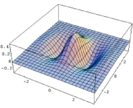
$f_{0}\,H_{40}$                      

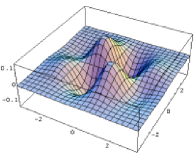
$f_{0}\,H_{31}$                      

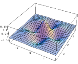
$f_{0}\,H_{22}$                      

Figure 1: Surface plots of Gaussians times individual hermite tensors, $f_{0}\,H_{n_{1}n_{2}}$ in two dimensions. Tensors $H_{04}$ and $H_{13}$ are images of $H_{40}$ and $H_{31}$ mirrored through the $z_{1}=z_{2}$ diagonal. Axis labels are in units of $\sqrt{2}\sigma_{i}$.

III.2 Hermite tensors

In the Edgeworth series (52) and (53), the cumulants $C$ are coefficients fixed by direct measurement, while the hermite tensors $H$ are, through eqs. (46)–(48) and explicit derivatives of (4), known functions of ${\mathbf{q}}$. Defining dimensionless variables

$$z_{i}=\frac{q_{i}}{\sigma_{i}}$$ (54)

which can also be written in terms of the usual radii as $z_{i}=\sqrt{2}\,q_{i}\,R_{ii}$, the lowest-order hermite tensors are, for the azimuthally symmetric out-side-long system,

$$h_{1}=H_{100} = \frac{z_{1}-\rho z_{3}}{\chi\sigma_{1}},$$ (55)

$$h_{2}=H_{010} = \frac{z_{2}}{\sigma_{2}},$$ (56)

$$h_{3}=H_{001} = \frac{z_{3}-\rho z_{1}}{\chi\sigma_{3}}.$$ (57)

Fourth-order derivatives (51) of the gaussian (4) yield,

$$H_{400} = h_{1}^{4}-6h_{1}^{2}\lambda_{11}^{-1}+3\lambda^{-1}_{11}\lambda^{-1}_{11},$$ (58)

$$H_{040} = h_{2}^{4}-6h_{2}^{2}\lambda_{22}^{-1}+3\lambda^{-1}_{22}\lambda^{-1}_{22},$$ (59)

$$H_{004} = h_{3}^{4}-6h_{3}^{2}\lambda_{33}^{-1}+3\lambda^{-1}_{33}\lambda^{-1}_{33},$$ (60)

$$H_{310} = h_{1}^{3}h_{2}-3h_{1}h_{2}\lambda_{11}^{-1},$$ (61)

$$H_{130} = h_{2}^{3}h_{1}-3h_{1}h_{2}\lambda_{22}^{-1},$$ (62)

$$H_{013} = h_{3}^{3}h_{2}-3h_{2}h_{3}\lambda_{33}^{-1},$$ (63)

$$H_{031} = h_{2}^{3}h_{3}-3h_{2}h_{3}\lambda_{22}^{-1},$$ (64)

$$H_{301} = h_{1}^{3}h_{3}-3h_{1}h_{3}\lambda_{11}^{-1}-3h_{1}^{2}\lambda_{13}^{-1}+3\lambda_{11}^{-1}\lambda_{13}^{-1},$$ (65)

$$H_{103} = h_{3}^{3}h_{1}-3h_{1}h_{3}\lambda_{33}^{-1}-3h_{3}^{2}\lambda_{13}^{-1}+3\lambda_{33}^{-1}\lambda_{13}^{-1},$$ (66)

$$H_{220} = h_{1}^{2}h_{2}^{2}-h_{1}^{2}\lambda_{22}^{-1}-h_{2}^{2}\lambda_{11}^{-1}+\lambda_{11}^{-1}\lambda_{22}^{-1},$$ (67)

$$H_{022} = h_{3}^{2}h_{2}^{2}-h_{3}^{2}\lambda_{22}^{-1}-h_{2}^{2}\lambda_{33}^{-1}+\lambda_{22}^{-1}\lambda_{33}^{-1},$$ (68)

$$H_{202} = h_{1}^{2}h_{3}^{2}-h_{1}^{2}\lambda_{33}^{-1}-h_{3}^{2}\lambda_{11}^{-1}-4h_{1}h_{3}\lambda_{13}^{-1}$$ (69)

$${}+\lambda_{11}^{-1}\lambda_{33}^{-1}+2\lambda_{13}^{-1}\lambda_{13}^{-1},$$

$$H_{211} = h_{1}^{2}h_{2}h_{3}-2h_{1}h_{2}\lambda_{13}^{-1}-h_{2}h_{3}\lambda_{11}^{-1},$$ (70)

$$H_{112} = h_{1}h_{2}h_{3}^{2}-2h_{2}h_{3}\lambda_{13}^{-1}-h_{1}h_{2}\lambda_{33}^{-1},$$ (71)

$$H_{121} = h_{1}h_{2}^{2}h_{3}-h_{2}^{2}\lambda_{13}^{-1}-h_{1}h_{3}\lambda_{22}^{-1}+\lambda_{22}^{-1}\lambda_{13}^{-1},$$ (72)

where the inverse cumulant elements $\lambda_{ij}^{-1}$ are functions of the parameters $\lambda_{i}$ and $\lambda_{ij}$ that can be read off from Eq. (32). The differences between various permutations of $(n_{1}n_{2}n_{3})$ above arise from the fact that $\lambda_{12}^{-1}=\lambda_{23}^{-1}=0$ for azimuthal symmetry.

Note that only one of the above hermite tensors can be written in terms of hermite polynomials at this level of generality, namely $H_{040}=H_{4}(z_{2})/\sigma_{2}^{4}$. Generally, the hermite tensors factorise into products of hermite polynomials $H_{n}(z_{i})\$ only if all Pearson coefficients $\rho_{ij}$ in the gaussian reference are zero,

$$H_{n_{1}n_{2}n_{3}}(\rho_{ij}{=}0)=\prod_{i=1}^{D}\frac{H_{n_{i}}(z_{i})}{\sigma_{i}^{n_{i}}}.$$ (73)

In sixth order, the tensors are generically

$$h_{ijklmn} = h_{i}h_{j}h_{k}h_{l}h_{m}h_{n}-h_{i}h_{j}h_{k}h_{l}\lambda_{mn}^{-1}[15]$$ (74)

$$+ h_{i}h_{j}\lambda_{kl}^{-1}\lambda_{mn}^{-1}[45]-\lambda_{ij}^{-1}\lambda_{kl}^{-1}\lambda_{mn}^{-1}[15]$$

where again the square brackets indicate the number of distinct index partitions. Sixth-order tensors $H_{n_{1}n_{2}n_{3}}$ can then be constructed from these as usual, for example

$$H_{600} = h_{1}^{6}-15h_{1}^{4}\lambda_{11}^{-1}+45h_{1}^{2}(\lambda_{11}^{-1})^{2}-15(\lambda_{11}^{-1})^{3}$$ (75)

which closely resembles the Hermite polynomial $H_{6}(z)=z^{6}-15z^{4}+45z^{2}-15$ but reduces to the latter only when $\rho_{ol}=0$ and hence $\lambda_{11}^{-1}=1/\sigma_{1}^{2}$.

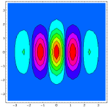
$f_{0}\,H_{60}$

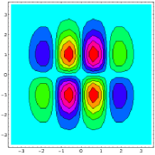
$f_{0}\,H_{51}$

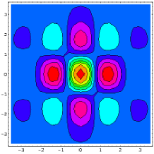
$f_{0}\,H_{42}$

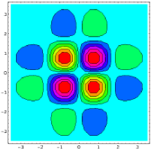
$f_{0}\,H_{33}$

Figure 2: Contour plots of Gaussians times individual sixth-order hermite tensors, $f_{0}\,H_{n_{1}n_{2}}$ in two dimensions. Red-green (light grey) areas represent hills while blue-red (dark grey) areas are valleys. Note how regions of phase space at a distance of several $\sigma_{i}$ from the peak are probed.

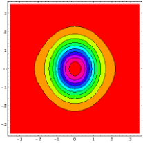
$H_{40}$

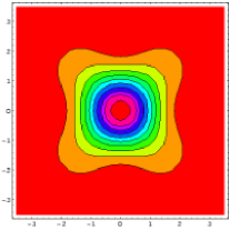
$H_{22}$

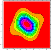
$H_{31}$

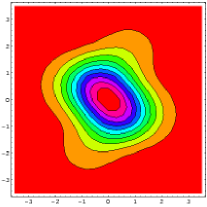
$H_{13}$

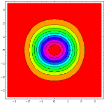
$H_{60}$

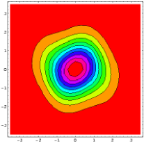
$H_{51}$

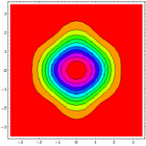
$H_{42}$

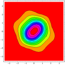
$H_{33}$

Figure 3: Contour plots of some individual terms in the Edgeworth expansion (52) of the form $f_{0}(1+F_{n_{1}n_{2}}C_{n_{1}n_{2}}H_{n_{1}n_{2}})$ Arbitrary and unrealistically large values of $C_{n_{1}n_{2}}=1$ for fourth order and $C_{n_{1}n_{2}}=2$ for sixth order were chosen, while the combinatoric prefactors $F_{n_{1}n_{2}}$ are fixed in (52). Both $H_{31}$ and $H_{13}$ are shown to exhibit their symmetry about the $z_{1}=z_{2}$ diagonal.

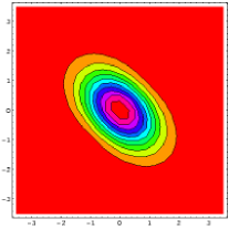
(a)

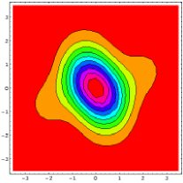
(d)

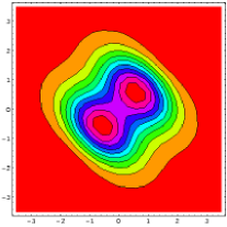
(b)

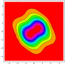
(e)

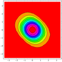
(c)

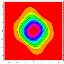
(f)

Figure 4: Combined terms for the two-dimensional Edgeworth: fourth-order terms only in (a) and (d); sixth-order terms only in (b) and (e); and all terms in (c) and (f). Fourth-order cumulants were set arbitrarily to 1 and sixth-order ones to 2. In (a)–(c), all cumulants are equal and nonzero, while in (d)–(f), cumulants $C_{04}$, $C_{13}$, $C_{06}$, $C_{15}$ and $C_{24}$ were set to zero in order to illustrate the possibility of asymmetric shapes.

III.3 A gallery of shapes

In Fig. 1, we show surface plots for individual fourth-order hermite tensors times the two-dimensional reference gaussian, $f_{0}H_{n_{1}n_{2}}$, with $\rho$ set to zero. As these are plotted in terms of $\sqrt{2}z_{i}=\sqrt{2}q_{i}/\sigma_{i}$ , the axes are scaled by the standard deviations, meaning that all gaussians with $\rho=0$ will be circular in $(z_{1},z_{2})$ plots. The individual hermite tensors clearly reflect the symmetry of their respective occupation number indices $n_{i}$ and probe different parts of the $(z_{1},z_{2})$ phase space as shown. Comparing the fourth-order terms of Fig. 1 with the sixth-order ones of Fig. 2, we note that the latter probe regions up to several $\sqrt{2}\,\sigma_{i}$.

In order to exhibit the influence of combinatoric factors, we show in Fig. 3 individual terms of the two-dimensional Edgeworth series (52) in the form $f_{0}({\mathbf{q}})(1+F_{n_{1}n_{2}}C_{n_{1}n_{2}}H_{n_{1}n_{2}}({\mathbf{q}}))$, where the combinatoric factors $F_{n_{1}n_{2}}$ are fixed in (52). All fourth- and sixth-order cumulants $C_{n_{1}n_{2}}$ have been set to 1.0 and 2.0 respectively. (This is obviously for illustrative purposes only; in real data, smaller values are expected and shapes will be more gaussian than those shown here.) The plots for $H_{31}$ and $H_{13}$ illustrate the correspondence between index permutation and symmetry about the $z_{1}=z_{2}$ axis. We note that the diagonal terms $H_{n0}$ have little influence on the overall shape, while the off-diagional ones have a larger effect, not least because of the combinatoric prefactors.

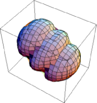
$400$                 

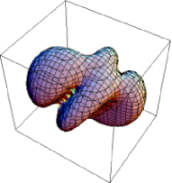
$310$                 

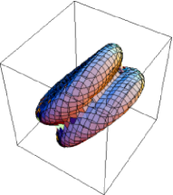
$301$                 

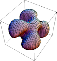
$220$                 

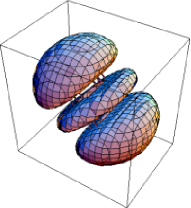
$202$                 

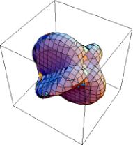
$121$                 

Figure 5: Typical contours for three-dimensional terms $f_{0}(1+F_{n_{1}n_{2}n_{3}}\,C_{n_{1}n_{2}n_{3}}\,H_{n_{1}n_{2}n_{3}})$ with indices as shown. Note that only a single contour is shown in each case.

Testing the influence of fourth- versus sixth-order terms, we show in Fig. 4 some “partial” two-dimensional Edgeworth series including only fourth-order terms, only sixth-order terms, and both orders; again, cumulants were set to the arbitrary values of 1 and 2 respectively.

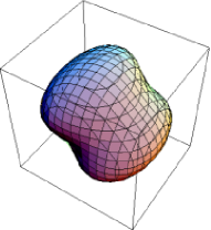
(a)                 

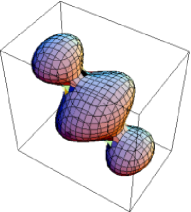
(b)                 

Figure 6: (a) Typical contour plot for combined Edgeworth with cumulants $C_{310}$, $C_{220}$, $C_{211}$ and their permutations set to 0.3 with all others (including 6th order) set to zero. (b) Combined Edgeworth with cumulants $C_{220}$, $C_{202}$, $C_{002}$, $C_{211}$, $C_{121}$, $C_{112}$ set to $0.15$ and all others to zero. Only single contours are shown.

In Fig. 5, a selection of shapes for individual terms $f_{0}({\mathbf{q}})(1+F_{n_{1}n_{2}n_{3}}C_{n_{1}n_{2}n_{3}}H_{n_{1}n_{2}n_{3}})$ of the three-dimensional Edgeworth expansion (53) is shown. While in the two-dimensional case full contour plots could be shown, the surfaces shown here in each case represent only a single contour. In Fig. 6, we show two examples with two selections of fourth-order cumulants nonzero; the shape obviously depends strongly on their selection and magnitude. Clearly, effects of the different cumulants on the overall shape often cancel out. We emphasize again that the shapes shown are for illustrative purposes only and do not represent real data.

IV Discussion

The multivariate Edgeworth expansions (52)–(53) appear to be a promising tool for quantitative shape analysis in HBT. While the real test will be to gauge their performance in actual data analysis, they do seem to have the right features and behaviour. A number of issues deserve further comment:

1. It has been noted previously Wie96a ; Wie96b that the traditional radii of a gaussian-shaped $R_{2}({\mathbf{q}})$ could be found by direct measurement rather than from fits. In the present formulation, this amounts to the direct measurement of the second-order cumulants $\lambda_{ij}$, which can be directly converted to “radius parameter” form via Eq. (32). Going beyond Refs. Wie96a ; Wie96b , we suggest that higher-order cumulants can be measured directly also.

2. Many people have rightly expressed concern that these radii do not adequately represent the true shapes and behaviour of HBT correlations. Our Edgeworth expansion confirms that such radii are clearly not the whole story, but that they do represent the appropriate lowest-order approximation (for gaussian reference) with respect to which nongaussian shapes should be measured.

3. We have demonstrated that it is imperative to write Edgeworth expansions in a fully multivariate way: the combinatoric prefactors $F_{n_{1}n_{2}n_{3}}$ in (53) are large for multivariate “off-diagonal” cumulants, while the influence of diagonal cumulants is strongly suppressed due to their small prefactors. The cumulant $C_{211}$, for example, has a weight 12 times larger than $C_{400}$, and indeed the entire expansion is dominated by the off-diagonal cumulants. Furthermore, even large diagonal cumulants do not change the shape much, as a glance at Fig. 3 will confirm.

4. Deviations from gaussian shapes are consistently quantified by the sign and magnitude of higher-order cumulants, which are identically zero for a null-case pure gaussian $f({\mathbf{q}})$. The Edgeworth expansion using these cumulants, while recreating the shape of $f({\mathbf{q}})$, therefore at the same time provides a quantitative framework for comparison of different shapes.

5. Operationally, we suggest a procedure of successive approximation, whereby in a first step all elements of the covariance matrix $\kappa_{ij}=\lambda_{ij}$ are measured, thereby determining all the $\sigma$’s and the Pearson coefficient; this is equivalent to the usual determination of radii. This is followed by measurement of the set of fourth-order cumulants $C_{n_{1}n_{2}n_{3}}$. The measured numbers for fourth-order cumulants then represent the basis for shape quantification and comparison. If statistics permit, sixth-order cumulants can be added as a further refinement.

6. The ${\mathbf{q}}$-cumulants proposed here are numbers rather than functions of ${\mathbf{q}}$. From the viewpoint of compactness of description, this will be an advantage compared to the shape decompositions in terms of spherical and cartesian harmonics Lis05a ; Dan05a , in which each coefficient is a function of $|{\mathbf{q}}|$. It may, however, in some cases be better to see the detail provided by such functions.

7. The procedure outlined above involves no fits. This represents a major advantage over fit-based quantification in two ways:

   Firstly: In three-dimensional analysis, typical fits are dominated by phase space, i.e. by the fact that there are many more bins at intermediate and large $|{\mathbf{q}}|$ than at small $|{\mathbf{q}}|$. This dominance suppresses the influence of the most interesting region on the $\chi^{2}$ for best-fit values of the parameters. In Ref. Egg06a , for example, we found that the regions of intermediate $|{\mathbf{q}}|$ dominated the shape and quality of various fits.

   Secondly, as shown in Fig. 2, cumulants are sensitive to the tails of distributions, and they will hence access the same information as these fits and parametrisations, but in a more direct and sensitive way. It is well known that a direct fit to a probability distribution that is close to gaussian is an ineffective and inaccurate way to quantify nongaussian deviations, while cumulants do so in the most direct way possible.

8. It remains to be seen how the proposed procedure fares when the practical experimental difficulties of finding $f({\mathbf{q}})$ and the higher-order cumulants come into play. Much will also depend on the size and accuracy of statistical errors. Fortunately, current sample sizes are large enough to warrant some optimism in this respect.

9. The traditional chaoticity parameter $\lambda$ remains undetermined within the present Edgeworth framework, because it cancels already in the definition (3) of $f({\mathbf{q}})$. For a given level of approximation (gaussian only, fourth-order cumulants, sixth-order), it and the overall normalisation factor $\gamma$ may be recovered afterwards by using (53) in a two-parameter fit mode using parametrisation

   $$\mbox{ }\ \ \ C_{2}({\mathbf{q}})=\gamma\left[1+\lambda f_{0}({\mathbf{q}})\left(\mbox{Edgeworth\ expansion}\,\right)\,\right]$$

   with the previously experimentally-determined radii and $C_{n_{1}n_{2}n_{3}}$ treated as constants, with $\gamma$ and $\lambda$ the fit parameters.

10. We note the importance of the parity argument $C_{2}(-{\mathbf{q}})=C_{2}({\mathbf{q}})$ in eliminating odd-order terms in the Edgeworth expansion. The parity argument falls away, however, in variables where this symmetry does not arise; for example, any one-dimensional Edgeworth expansion involving only positive differences (e.g. in $q_{\rm inv}$) would have to include third- and fifth-order terms.

    A corollary of the parity argument is that three-dimensional correlations may not be represented in terms of positive absolute values of the components $(q_{o},q_{s},q_{l})$ as this destroys the underlying symmetries. The best one can do to improve statistics is to combine bins that map onto each other under the transformation ${\mathbf{q}}\to-{\mathbf{q}}$ and thereby eliminate four of the eight octants in the three-dimensional $(q_{o},q_{s},q_{l})$-space.

11. In the present formulation, any dependence on average pair momentum ${\mathbf{K}}$ resides in the cumulants: all $\kappa_{ijk\ldots}$, including the traditional radii and the Pearson coefficient, are in principle functions of ${\mathbf{K}}$.

12. The Edgeworth analysis set out in this contribution is based on a gaussian reference $f_{0}$. Shapes that differ significantly from gaussian will not be described well in either the Edgeworth framework or the spherical or cartesian harmonics frameworks. One should not, for example, expect power laws such as a pure Coulomb wavefunction (whose square tails off like $|{\mathbf{q}}|^{-2}$) to work in a gaussian-based Edgeworth expansion. Indeed, it is known that large cumulants can lead to a situation where the truncated Edgeworth expansion of $f({\mathbf{q}})$ becomes negative in some regions. It is therefore suitable only for shapes that do not deviate strongly from gaussians; for strong deviations, other expansions will become a necessity.

13. The Edgeworth framework is easily extended to the case of nonidentical particles. In that case, cumulants of all orders will have to be measured. It may well be that the fluctuations of lower-order quantities render the measurement of higher-order cumulants impossible, and great care will clearly have to be taken.

References

• (1) G. Goldhaber, S. Goldhaber, W. Lee and A. Pais, Phys. Rev. 120, 300 (1960).
• (2) EHS/NA22 Collaboration, N. M. Agababyan et al., Z. Phys.  C 71 (1996) 405.
• (3) H.C. Eggers, B. Buschbeck and F.J. October, Phys. Lett. B635, 280 (2006); hep-ex/0601039.
• (4) Z. Chajecki, T.D. Gutierrez, M.A. Lisa and M. Lopez-Noriega (STAR Collaboration), in: 21st Winter Workshop on Nuclear Dynamics, Breckenridge CO, February 2005, nucl-ex/0505009.
• (5) S. Hegyi and T. Csörgő, Proc. Budapest Workshop on Relativistic Heavy Ion Collisions, preprint KFKI–1993-11; T. Csörgő, in: Soft Physics and Fluctuations, Proc. Cracow Workshop on Multiparticle Production, Cracow, 1993, ed. A. Białas, K. Fiałkowski, K. Zalewski and R.C. Hwa, World Scientific (1994), p. 175.
• (6) T. Csörgő and S. Hegyi, Phys. Lett. B489, 15 (2000).
• (7) D.A. Brown and P. Danielewicz, Phys. Lett. B398, 252 (1997); nucl-th/9701010.
• (8) D.A. Brown and P. Danielewicz, Phys. Rev. C57, 2474 (1998); nucl-th/9712066.
• (9) D.A. Brown et al., Phys. Rev. C72 054902 (2005); nucl-th/0507015.
• (10) P. Danielewicz and S. Pratt, Phys. Lett. B618, 60 (2005); nucl-th/0501003.
• (11) P. Lipa, H.C. Eggers and B. Buschbeck, Phys. Rev. D 53, 4711 (1996); hep-ph/9604373.
• (12) A. Stuart and J.K. Ord Kendall’s Advanced Theory of Statistics, 5th edition Vol. 1, Oxford University Press, New York (1987).
• (13) P. Carruthers, H.C. Eggers, and I. Sarcevic, Phys. Lett. B254, 258 (1991).
• (14) U.A. Wiedemann and U. Heinz, Phys. Rev. C56, 610 (1996); nucl-th/9610043.
• (15) U.A. Wiedemann and U. Heinz, Phys. Rev. C56, 3265 (1996); nucl-th/9611031.
• (16) B.R. Schlei, D. Strottman and N. Xu, Phys. Lett. B420, 1 (1998); nucl-th/9702011.
• (17) S. Chapman, J.R. Nix and U. Heinz, Phys. Rev. C52, 2694 (1995); nucl-th/9505032.
• (18) J.M. Chambers, Biometrika 54, 367 (1967).
• (19) O.E. Barndorff-Nielsen, Parametric Statistical Models and Likelihood, Lecture Notes in Statistics Vol. 50, Springer (1988).