Relativistic Dynamics of Non-ideal Fluids: Viscous and heat-conducting fluids
II. Transport properties and microscopic description of relativistic nuclear matter

Abstract

In the causal theory of relativistic dissipative fluid dynamics, there are conditions on the equation of state and other thermodynamic properties such as the second-order coefficients of a fluid that need to be satisfied to guarantee that the fluid perturbations propagate causally and obey hyperbolic equations. The second-order coefficients in the causal theory, which are the relaxation times for the dissipative degrees of freedom and coupling constants between different forms of dissipation (relaxation lengths), are presented for partonic and hadronic systems. These coefficients involves relativistic thermodynamic integrals. The integrals are presented for general case and also for different regimes in the temperature–chemical potential plane. It is shown that for a given equation of state these second-order coefficients are not additional parameters but they are determined by the equation of state. We also present the prescription on the calculation of the freeze-out particle spectra from the dynamics of relativistic non-ideal fluids.

I Introduction

Transport properties of relativistic hot and dense matter are important in many physical situations such as in nuclear physics, astrophysics and cosmology. The hot and dense relativistic matter is produced in high energy relativistic nuclear reactions such as those in heavy-ion experiments while the hot matter is believed to have existed in the early universe and the dense matter might be found in the quark stars and neutron stars. The transport properties of a system out of equilibrium are governed by transport coefficients which relate flows to thermodynamic forces. These coefficients characterize the magnitude of the response of the system (flow) to a certain disturbance (thermodynamic force).

The space-time evolution of the produced matter in high energy nuclear collisions can be studied using relativistic fluid dynamics. In order to take into account non-equilibrium (dissipative) effects we need to use relativistic non-ideal fluid dynamics. We consider the causal theory of relativistic fluids as presented in paper I AMI .

In the high energy heavy ion collisions the rapid evolution of the fluid is governed by dissipative effects via transport coefficients such as the shear and bulk viscosities, the thermal conductivity, the diffusion coefficients, etc. These transport coefficients are generally calculated via the use of kinetic theory and thereby imply the knowledge of a collision term. The collision term must be a representation of the hot and dense matter at hand.

In addition to the standard transport coefficients the causal theory contains other thermodynamic functions, namely the second-order coefficients. These coefficients, in combination with the standard transport coefficients, are related to the relaxation times and relaxation length for various dissipative processes. The relaxation length results from the coupling between the heat flux and viscous processes. These second-order coefficients are given by complicated thermodynamic integrals. In this work we will present the second-order transport coefficients in detail for future applications in the description of the relativistic dynamics of heat-conducting and viscous matter produced in high energy nuclear collisions.

In addition to the knowledge of the transport coefficients and second-order thermodynamic function we need to know how to determine the form of the equation of state. Knowledge of the equation of state is needed for analyzing many important physical situations such as supernova explosions and neutron star formation, high energy nuclear collisions, and the study of quark-hadron phase transition in the early universe. Recent developments in heavy ion collision experiments can reveal the form of the equation of state of the nuclear matter. The physics involved in such collisions is highly complex and it is highly nontrivial matter to extract equation of state information from such a complex dynamical situation.

In this paper we would like to investigate the influence of the equation of state on the transport properties of the relativistic hot and dense matter. The equation of state in the hadronic phase is derived from the Walecka model of nuclear matter and in the QGP phase we use the MIT Bag model. In the mixed phase we employ the Gibbs construction for the phase equilibria.

The rest of the paper is organized as follows: In Section II we present the moments of relativistic Boltzmann equation in terms of the relativistic thermodynamic integrals. In Section III we present the 14-Field Theory from the microscopic considerations. We consider small deviations from equilibrium and employ the Grad’s 14 moment method. In Section IV we present the second order entropy 4-current in terms of the relaxation and coupling coefficients which are collectively referred to as the second order coefficients. In Section V we present the EoS considered in this work. In Section VI we present the freeze-out prescription which takes into account the dissipative corrections. In Appendix A we present the relativistic thermodynamic integrals. In Appendix B we present the various limiting cases of the thermodynamic integrals. In Appendix C we present the ultra-relativistic thermodynamic integrals. In Appendix D we present the relativistic thermodynamic integrals at zero temperature.

Our units are $\hbar=c=k_{\rm B}=1$. The metric tensor is $g^{\mu\nu}=\mbox{diag}(+,-,-,-)$. The scalar product of two 4-vectors $a^{\mu},\,\,b^{\mu}$ is denoted by $a^{\mu}\,g_{\mu\nu}\,b^{\nu}\equiv a^{\mu}\,b_{\mu}$, and the scalar product of two 3-vectors ${a}$ and ${b}$ by $\mbox{\boldmath${a}$}\cdot\mbox{\boldmath${b}$}$. The notations $A^{(\alpha\beta)}\equiv(A^{\alpha\beta}+A^{\beta\alpha})/2$ and $A^{[\alpha\beta]}\equiv(A^{\alpha\beta}-A^{\beta\alpha})/2$ denote symmetrization and antisymmetrization, respectively. The notation $A^{\langle\alpha\beta\rangle}=[\bigtriangleup_{\mu}^{(\alpha}\bigtriangleup_{\nu}^{\beta)}-1/3\bigtriangleup^{\alpha\beta}\bigtriangleup_{\mu\nu}]A^{\mu\nu}$ denotes the trace-free part of $A^{\mu\nu}$. The 4-derivative is denoted by ${\partial}_{\alpha}\equiv{\partial}/{\partial}x^{\alpha}$. An overdot denotes $\dot{A}=u^{\lambda}{\partial}_{\lambda}A$.

II The Relativistic Transport Equation and the Moment Equations

The transport equation gives the rate of change of the distribution function in time and in space due to the particle interactions. The distribution function can in principle be solved from the transport equation. Here we limit ourselves to cases valid for dilute systems where binary collisions dominate. In trying to study high energy nuclear reactions we need to know the properties of many-particle system. While the properties of such a system depends upon the interactions of the constituent particles and external constraints in kinetic theory in the macroscopic level such a system is described by the net conserved densities, the energy density, hydrodynamic velocity and dissipative quantities. Thus the resulting fluid dynamic equations can be considered as an effective kinetic theory. The results should be compared with other theories which goes beyond dilute systems to check the deviations.

The relativistic Boltzmann transport equation for the invariant on-shell phase space density $f(x,p)$ is

$$p^{\mu}{\partial}_{\mu}f(x,p)=p^{\mu}u_{\mu}\mbox{D}f(x,p)+p^{\mu}\bigtriangledown_{\mu}f(x,p)={\mathcal{C}}[f(x,p)]~{},$$ (1)

where ${\mathcal{C}}[f]$ stands for the collision term. Here $\mbox{D}=u^{\mu}{\partial}_{\mu}$ is the covariant time derivative and $\bigtriangledown_{\mu}=\bigtriangleup^{\mu\nu}{\partial}_{\nu}$ is the covariant gradient operator. Furthermore, $\bigtriangleup^{\mu\nu}=g^{\mu\nu}-u^{\mu}u^{\nu}$ is the projection tensor and $u^{\mu}=(\gamma,\,\gamma\mbox{\boldmath${v}$})$ is the 4-velocity where $\gamma=\sqrt{1-{\bf v}^{2}}$ and the three–velocity of a particle is ${\bf v}\equiv{\bf p}/p^{0}$. The four velocity is normalized such that $u^{\mu}u_{\mu}=1$. The four momentum is $p^{\mu}=(p^{0},{\bf p})$ where $p^{0}=E=\sqrt{{\bf p}^{2}+m^{2}}$ is the relativistic energy of the particle and $m$ is the mass of the particle. Eq. (1) describes the time evolution of the single particle distribution function $f(x,p)$. The local equilibrium distribution function has the form

$$f^{\rm eq}(x,p)=A_{0}{1\over e^{\beta_{\mu}p^{\mu}-\alpha}-a}$$ (2)

where $A_{0}=g/(2\pi)^{3}$ and $a$ corresponds to the statistics of Boltzmann $(a=0)$, Bose $(a=+1)$, and Fermi $(a=-1)$ distributions. Also the degeneracy $g=(2J+1)$ where $J$ is the spin of the particle, $\beta_{\mu}=\beta u_{\mu}$, $\alpha=\beta\mu$ with $\beta=1/T$ the inverse temperature, and $\mu$ is the chemical potential.

Let us define the first five moments of the distribution function $f(x,p)$ by

$$N^{\mu}(x) \equiv \int f(x,p)p^{\mu}\mbox{d}w~{},$$ (3)

$$T^{\mu\nu}(x) \equiv \int f(x,p)p^{\mu}p^{\nu}\mbox{d}w~{},$$ (4)

$$F^{\lambda\mu\nu}(x) \equiv \int f(x,p)p^{\lambda}p^{\mu}p^{\nu}\mbox{d}w~{},$$ (5)

$$R^{\alpha\beta\mu\nu}(x) \equiv \int f(x,p)p^{\alpha}p^{\beta}p^{\mu}p^{\nu}\mbox{d}w~{},$$ (6)

$$Q^{\alpha\beta\mu\nu\rho}(x) \equiv \int f(x,p)p^{\alpha}p^{\beta}p^{\mu}p^{\nu}p^{\rho}\mbox{d}w~{},$$ (7)

where

$$\mbox{d}w\equiv{\mbox{d}^{3}{\bf p}\over p^{0}}.$$ (8)

For the equilibrium distribution function $f^{{\rm eq}}(x,p)$, Eq. (2), the five moments can be written as

$$N^{\mu}_{\rm eq} = {\cal I}_{10}u^{\mu}~{},$$ (9)

$$T^{\mu\nu}_{\rm eq} = {\cal I}_{20}u^{\mu}u^{\nu}-{\cal I}_{21}\bigtriangleup^{\mu\nu}~{},$$ (10)

$$F^{\lambda\mu\nu}_{\rm eq} = {\cal I}_{30}u^{\lambda}u^{\mu}u^{\nu}-3{\cal I}_{31}\bigtriangleup^{(\lambda\mu}u^{\nu)}~{},$$ (11)

$$R^{\alpha\beta\mu\nu}_{\rm eq} = {\cal I}_{40}u^{\alpha}u^{\beta}u^{\mu}u^{\nu}-6{\cal I}_{41}\bigtriangleup^{(\alpha\beta}u^{\mu}u^{\nu)}+3{\cal I}_{42}\bigtriangleup^{(\alpha\beta}\bigtriangleup^{\mu\nu)}$$ (12)

$$Q^{\alpha\beta\mu\nu\rho}_{\rm eq} = {\cal I}_{50}u^{\alpha}u^{\beta}u^{\mu}u^{\nu}u^{\rho}-10{\cal I}_{51}\bigtriangleup^{(\alpha\beta}u^{\mu}u^{\nu}u^{\rho)}+15{\cal I}_{52}\bigtriangleup^{(\alpha\beta}\bigtriangleup^{\mu\nu}u^{\rho)}$$ (13)

where the ${\cal I}_{nk}$ are the equilibrium thermodynamic functions and are presented in Appendix A. Various contractions of the above equations produce useful relations such as

$$u_{\mu}N_{{\rm eq}}^{\mu} = {\cal I}_{10}\equiv n~{},~{}~{}~{}~{}~{}u_{\mu}u_{\nu}T_{{\rm eq}}^{\mu\nu}={\cal I}_{20}\equiv\varepsilon~{},~{}~{}~{}~{}~{}{T_{{\rm eq}}}^{\mu}_{\mu}={\cal I}_{20}-3{\cal I}_{21}\equiv\varepsilon-3p~{},$$ (14)

$$u_{\lambda}{F_{{\rm eq}}}^{\lambda\nu}_{\nu} = {\cal I}_{30}-3{\cal I}_{31}=m^{2}n~{},~{}~{}~{}~{}~{}u_{\alpha}u_{\beta}{R_{{\rm eq}}}^{\alpha\beta\nu}_{\nu}={\cal I}_{40}-3{\cal I}_{41}=m^{2}\varepsilon~{}.$$ (15)

Corresponding to the five moments are the five auxiliary moments of $\Delta(x,p)f(x,p)$, which arises due to variations in the distribution function,

$$\tilde{N}^{\mu}(x) \equiv \int\Delta(x,p)f(x,p)p^{\mu}\mbox{d}w~{},$$ (16)

$$\tilde{T}^{\mu\nu}(x) \equiv \int\Delta(x,p)f(x,p)p^{\mu}p^{\nu}\mbox{d}w~{},$$ (17)

$$\tilde{F}^{\lambda\mu\nu}(x) \equiv \int\Delta(x,p)f(x,p)p^{\lambda}p^{\mu}p^{\nu}\mbox{d}w~{},$$ (18)

$$\tilde{R}^{\alpha\beta\mu\nu}(x) \equiv \int\Delta(x,p)f(x,p)p^{\alpha}p^{\beta}p^{\mu}p^{\nu}\mbox{d}w~{}.$$ (19)

$$\tilde{Q}^{\alpha\beta\mu\nu\rho}(x) \equiv \int\Delta(x,p)f(x,p)p^{\alpha}p^{\beta}p^{\mu}p^{\nu}p^{\rho}\mbox{d}w~{},$$ (20)

where $\Delta(x,p)\equiv 1+aA_{0}^{-1}f(x,p)$. For the equilibrium distribution function, Eq. (2), and $\Delta^{{\rm eq}}(x,p)f^{{\rm eq}}(x,p)$ the auxiliary moments can be written as

$$\tilde{N}^{\mu}_{\rm eq} = {\cal J}_{10}u^{\mu}~{},$$ (21)

$$\tilde{T}^{\mu\nu}_{\rm eq} = {\cal J}_{20}u^{\mu}u^{\nu}-{\cal J}_{21}\bigtriangleup^{\mu\nu}~{},$$ (22)

$$\tilde{F}^{\lambda\mu\nu}_{\rm eq} = {\cal J}_{30}u^{\lambda}u^{\mu}u^{\nu}-3{\cal J}_{31}\bigtriangleup^{(\lambda\mu}u^{\nu)}~{},$$ (23)

$$\tilde{R}^{\alpha\beta\mu\nu}_{\rm eq} = {\cal J}_{40}u^{\alpha}u^{\beta}u^{\mu}u^{\nu}-6{\cal J}_{41}\bigtriangleup^{(\alpha\beta}u^{\mu}u^{\nu)}+3{\cal J}_{42}\bigtriangleup^{(\alpha\beta}\bigtriangleup^{\mu\nu)}$$ (24)

$$\tilde{Q}^{\alpha\beta\mu\nu\rho}_{\rm eq} = {\cal J}_{50}u^{\alpha}u^{\beta}u^{\mu}u^{\nu}u^{\rho}-10{\cal J}_{51}\bigtriangleup^{(\alpha\beta}u^{\mu}u^{\nu}u^{\rho)}+15{\cal J}_{52}\bigtriangleup^{(\alpha\beta}\bigtriangleup^{\mu\nu}u^{\rho)}~{}.$$ (25)

where the relativistic thermodynamic integrals ${\cal J}_{nk}$ are also presented in Appendix A. Note that by Eq. (A) the ${\cal J}_{nk}$ can be related to the ${\cal I}_{nk}$, for example

$${\cal J}_{21}={{\cal I}_{10}\over\beta},\;\;\;\;{\cal J}_{31}={({\cal I}_{20}+{\cal I}_{21})\over\beta},\;\;\;\;{\cal J}_{41}={({\cal I}_{30}+2{\cal I}_{31})\over\beta},\;\;\;\;{\cal J}_{42}={{\cal I}_{31}\over\beta}~{}.$$ (26)

Also by Eq. (177) the ${\cal J}_{nk}$ can be obtained as differentiation of the ${\cal I}_{nk}$ with respect to $\alpha$ and $\beta$.

As in the case of the ${\cal I}_{nk}$ similar contractions of the ${\cal J}_{nk}$ leads to similar relations, Eqs. (14)–(15), with the ${\cal I}_{nk}$ now replaced by the ${\cal J}_{nk}$. For later reference we define the entropy 4-current in kinetic theory as

$$S^{\mu}(x)=-\int\mbox{d}w\,p^{\mu}\left\{f(x,p)\ln\left(A_{0}^{-1}f(x,p)\right)-a^{-1}A_{0}\Delta(x,p)\ln\Delta(x,p)\right\}~{},$$ (27)

and we introduce a quantity

$$h_{i}\equiv{(\varepsilon+p)\over n_{i}}={w\over n_{i}}={{\cal J}_{31}\over{\cal J}_{21}}~{},$$ (28)

where $w=\varepsilon+p$, as the enthalpy per net conserved $i$th charge. Since in our case we are considering one such charge, namely the net baryon number, $h$ denotes the enthalpy per net baryon. Similarly one defines $s/n$ as the entropy per net baryon.

III The 14-Field Theory of Non-equilibrium Relativistic Fluid Dynamics

III.1 Small deviations from thermal equilibrium

For a gas that departs slightly from the local thermal equilibrium, we may write the distribution function as

$$f(x,p)=f^{\rm eq}(x,p)\left\{1+\Delta^{\rm eq}(x,p)\phi(x,p)\right\}~{},$$ (29)

where $\phi(x,p)$ is the deviation function to be discussed in the next subsection. Substitution of Eq. (29) into Eqs. (3), (4), and (27) yields

$$N^{\mu}(x) = N^{\mu}_{\rm eq}(x)+\delta N^{\mu}(x)~{},$$ (30)

$$T^{\mu\nu}(x) = T^{\mu\nu}_{\rm eq}(x)+\delta T^{\mu\nu}(x)~{},$$ (31)

$$S^{\mu}(x) = S^{\mu}_{\rm eq}(x)+\delta S^{\mu}(x)~{},$$ (32)

where $N^{\mu}_{\rm eq}$, $T^{\mu\nu}_{\rm eq}$, and $S^{\mu}_{\rm eq}$ have the ideal fluid (equilibrium) form, and

$$\delta N^{\mu}(x) = \int f^{\rm eq}(x,p)\Delta^{\rm eq}(x,p)\phi(x,p)p^{\mu}\mbox{d}w~{},$$ (33)

$$\delta T^{\mu\nu}(x) = \int f^{\rm eq}(x,p)\Delta^{\rm eq}(x,p)\phi(x,p)p^{\mu}p^{\nu}\mbox{d}w~{}.$$ (34)

For the entropy, expanding the term in the curly brackets in Eq. (27) up to terms of second order in deviations $\phi(x,p)$ (cf. Section IV) leads to

$$\delta S^{\mu}(x) = S^{\mu}(x)-S^{\mu}_{\rm eq}(x)$$ (35)

$$=-\int\left[\alpha(x)-\beta_{\nu}(x)p^{\nu}\right]f^{\rm eq}(x,p)\Delta^{\rm eq}(x,p)\phi(x,p)p^{\mu}\mbox{d}w$$

$$-\frac{1}{2}\int f^{\rm eq}(x,p)\Delta^{\rm eq}(x,p)\left(\phi(x,p)\right)^{2}p^{\mu}\mbox{d}w+\cdot\cdot\cdot$$

which corresponds to the phenomenological expression

$$\delta S^{\mu}(x)=-\alpha(x)\delta N^{\mu}(x)+\beta_{\nu}(x)\delta T^{\mu\nu}(x)+Q^{\mu}(x)~{},$$ (36)

with

$$Q^{\mu}(x)=-\frac{1}{2}\int f^{\rm eq}(x,p)\Delta^{{\rm eq}}(\phi(x,p))^{2}p^{\mu}\mbox{d}w+\cdot\cdot\cdot~{}.$$ (37)

now explicitly defined in kinetic theory. The five parameters $\alpha$ and $\beta_{\mu}$ which describe the nearby equilibrium state can be specified by matching the equilibrium state to the actual state. This is done by the prescription that the net charge density and energy density are completely determined by the equilibrium distribution function. That is, we impose the following conditions:

$$n \equiv \int\mbox{d}wp^{\mu}u_{\mu}f(x,p)=n_{\rm eq}\equiv\int\mbox{d}wp^{\mu}u_{\mu}f^{\rm eq}(x,p)~{},$$ (38)

$$\varepsilon \equiv \int\mbox{d}w(p^{\mu}u_{\mu})^{2}f(x,p)=\varepsilon_{\rm eq}\equiv\int\mbox{d}w(p^{\mu}u_{\mu})^{2}f^{\rm eq}(x,p)~{}.$$ (39)

Then $p(\varepsilon,n)\equiv p(\varepsilon_{\rm eq},n_{\rm eq})$ is the actual equation of state. The above matching conditions also implies

$$u_{\mu}\delta N^{\mu}=u_{\mu}u_{\nu}\delta T^{\mu\nu}=0~{}.$$ (40)

It then follows from Eqs. (36) and (37) that

$$u_{\mu}\delta S^{\mu}=u_{\mu}Q^{\mu}\leq 0~{},$$ (41)

confirming that equilibrium maximizes the entropy density under the above constraints, Eq. (40), on particle and energy densities , and that $S_{\rm eq}^{\mu}$ and $T^{\mu\nu}_{\rm eq}$ give the entropy and thermodynamical pressure correctly to first order in deviations. To fix the hydrodynamic velocity we may choose either the Eckart’s or Landau-Lifshitz’ definition of the 4-velocity. The former case implies

$$\bigtriangleup^{\mu\nu}N_{\nu}=\int\mbox{d}w\bigtriangleup^{\mu\nu}p_{\nu}f^{\rm eq}(x,p)=0~{},$$ (42)

and the latter case implies

$$\bigtriangleup^{\mu\nu}T_{\nu\sigma}u^{\sigma}=\int\mbox{d}w\bigtriangleup^{\mu\nu}p_{\nu}p_{\sigma}u^{\sigma}f^{\rm eq}(x,p)=0~{}.$$ (43)

In finding the equations for non-ideal fluid dynamics from microscopic/kinetic theory there are basically two approaches which lead to linearized transport equations: the Chapman–Enskog approximation Chapman and Grad’s 14–moment approximation HG . In the Chapman-Enskog method one solves a linearized Boltzmann equation for $f(x,p)$ which is linearized by assuming that the function $\phi(x,p)$ that measures deviation from local equilibrium is small. Terms which are non-linear in $\phi(x,p)$ and also the relative variation over a mean free path are neglected. One then uses the conservation laws $\partial_{\mu}N^{\mu}\equiv\partial_{\mu}T^{\mu\nu}\equiv 0$ to express the time derivatives D of the thermodynamical variables and the four–velocity (hence $\mbox{D}f^{\rm eq}(x,p)$) in terms of spatial gradients $\bigtriangledown_{\mu}$ of $\alpha(x)$ and $\beta_{\mu}(x)$, correct to first order. Substitution into the kinetic expressions (cf. Eq. (1)) connects these gradients to heat flow, diffusion and viscosity. The second approximation which is based on the moment method is more general and has a wide scope of applicability. It will be discussed in the following section.

III.2 Grad’s 14–Moment Approximation

In the phenomenological theories of relativistic non-ideal fluid dynamics by Eckart CE and by Landau and Lifshitz LL (see AMI for details], instantaneous propagation of heat and viscous signals (acausality problem) remained a puzzle for many years. However, in 1966, I. Müller IM traced the origin of the difficulty to the neglect of terms of second order in heat flux and viscosity in the conventional theory’s expression for the entropy. Restoring these terms, Müller was led to a modified system of phenomenological equations which was consistent with the linearized form of Grad’s kinetic equations. Müller’s theory was rediscovered and extended to relativistic fluids by Israel and Stewart IS in the 1970’s.

The progress made in phenomenology in getting rid of the acausality problem can also be made from kinetic theory. The analogous paradox in non-relativistic kinetic theory was resolved by Grad HG , who showed in 1949 how transient effects could be treated by employing the method of moments instead of the Chapman-Enskog normal solution. Suitable truncation of the moment equations gave a closed system of differential equations which turned out to be hyperbolic, with propagation speeds of the order of the speed of sound. The relativistic version of Grad’s method was developed by Israel and Stewart IS .

In phenomenology we seek a truncated hydrodynamical linearized description of small departures from equilibrium in which only the 14 variables $N^{\mu}(x)$ and $T^{\mu\nu}(x)$ appear. The microscopic counterpart of this is a truncated description in which the function

$$y(x,p)=\ln\left[A_{0}^{-1}f(x,p)/\Delta(x,p)\right]~{},$$ (44)

differs from any nearby local equilibrium value

$$y_{\rm eq}(x,p)=\alpha(x)-\beta_{\mu}(x)p^{\mu}~{},$$ (45)

by a function of momenta specifiable by 14 dynamic variables. The truncated description is accomplished by postulating the relativistic Grad’s 14–moment approximation IS ; HG , or variational method deGroot , that $y-y_{\rm eq}$ can be approximated by a quadratic function in momenta

$$\phi(x,p)\equiv y(x,p)-y_{\rm eq}(x,p)=\epsilon(x)-\epsilon_{\mu}(x)p^{\mu}+\epsilon_{\mu\nu}(x)p^{\mu}p^{\nu}+...~{},$$ (46)

or

$$y(x,p)=(\alpha+\epsilon(x))-(\beta_{\mu}+\epsilon_{\mu}(x))p^{\mu}+\epsilon_{\mu\nu}(x)p^{\mu}p^{\nu}+...~{},$$ (47)

where $\epsilon(x),\,\epsilon_{\mu}(x)$, and $\epsilon_{\mu\nu}(x)$ are small. Without loss of generality $\epsilon_{\mu\nu}(x)$ may be assumed traceless, since its trace can be absorbed in redefinition of $\epsilon(x)$. The non-equilibrium distribution function is given by Eq. (29) and it depends on the 14 variables $\alpha+\epsilon\,,\beta_{\mu}+\epsilon_{\mu}$, and $\epsilon_{\mu\nu}$. While five of these determine the equilibrium state the other nine variables are related to the dissipative fluxes. Inserting the expression for $f(x,p)$, Eq. (29), into the kinetic expressions for $N^{\mu}$ and $T^{\mu\nu}$, Eqs. (3) and (4), we then have

$$N^{\mu} = N^{\mu}_{\rm eq}+\epsilon\int\mbox{d}wf^{\rm eq}(x,p)\Delta^{\rm eq}(x,p)p^{\mu}$$ (48)

$$-\epsilon_{\nu}\int\mbox{d}wf^{\rm eq}(x,p)\Delta^{\rm eq}(x,p)p^{\mu}p^{\nu}+\epsilon_{\nu\lambda}\int\mbox{d}wf^{\rm eq}(x,p)\Delta^{\rm eq}(x,p)p^{\mu}p^{\nu}p^{\lambda}$$

$$T^{\mu\nu} = T^{\mu\nu}_{\rm eq}+\epsilon\int\mbox{d}wf^{\rm eq}(x,p)\Delta^{\rm eq}(x,p)p^{\mu}p^{\nu}-\epsilon_{\lambda}\int\mbox{d}wf^{\rm eq}(x,p)\Delta^{\rm eq}(x,p)p^{\mu}p^{\nu}p^{\lambda}$$ (49)

$$+\epsilon_{\lambda\rho}\int\mbox{d}wf^{\rm eq}(x,p)\Delta^{\rm eq}(x,p)p^{\mu}p^{\nu}p^{\lambda}p^{\rho}$$

$$F^{\sigma\mu\nu} = F^{\sigma\mu\nu}_{\rm eq}+\epsilon\int\mbox{d}wf^{\rm eq}(x,p)\Delta^{\rm eq}(x,p)p^{\sigma}p^{\mu}p^{\nu}-\epsilon_{\lambda}\int\mbox{d}wf^{\rm eq}(x,p)\Delta^{\rm eq}(x,p)p^{\sigma}p^{\mu}p^{\nu}p^{\lambda}$$ (50)

$$+\epsilon_{\lambda\rho}\int\mbox{d}wf^{\rm eq}(x,p)\Delta^{\rm eq}(x,p)p^{\sigma}p^{\mu}p^{\nu}p^{\lambda}p^{\rho}$$

Then by Eqs. (16)-(19) one can write the non-equilibrium part of the number four current, the energy-momentum tensor and the fluxes as

$$\delta N^{\mu} = \epsilon\tilde{N}^{\mu}_{\rm eq}-\epsilon_{\lambda}\tilde{T}^{\mu\lambda}_{\rm eq}+\epsilon_{\lambda\nu}\tilde{F}^{\lambda\mu\nu}_{\rm eq}~{},$$ (51)

$$\delta T^{\mu\nu} = \epsilon\tilde{T}^{\mu\nu}_{\rm eq}-\epsilon_{\lambda}\tilde{F}^{\lambda\mu\nu}_{\rm eq}+\epsilon_{\lambda\rho}\tilde{R}^{\lambda\rho\mu\nu}_{\rm eq}~{},$$ (52)

$$\delta F^{\sigma\mu\nu} = \epsilon\tilde{F}^{\sigma\mu\nu}_{\rm eq}-\epsilon_{\lambda}\tilde{R}^{\sigma\mu\nu\lambda}_{\rm eq}+\epsilon_{\lambda\rho}\tilde{Q}^{\sigma\mu\nu\lambda\rho}_{\rm eq}~{}.$$ (53)

From the definitions of the dissipative fluxes, namely the particle drift flux $V^{\mu}=\bigtriangleup^{\mu}_{\nu}\delta N^{\nu}$, the energy flux $W^{\mu}=\bigtriangleup^{\mu}_{\nu}u_{\rho}\delta T^{\nu\rho}$, the heat flux $q^{\mu}=W^{\mu}-hV^{\mu}$, the bulk viscous pressure $\Pi\equiv-{1\over 3}\bigtriangleup_{\mu\nu}\delta T^{\mu\nu}$ and the shear stress tensor $\pi^{\mu\nu}\equiv\delta T^{\langle\mu\nu\rangle}$ and the matching conditions, Eq. (40), one then obtains the 14 variables $\alpha+\epsilon\,,\beta^{\mu}+\epsilon^{\mu}$, and $\epsilon^{\mu\nu}$ in terms of the macroscopic fields $n,\,\varepsilon,\,u^{\mu},\,\Pi,\,q^{\mu}$, and $\pi^{\mu\nu}$ IS

$$\epsilon_{\mu\nu} = {\cal A}_{2}(3u_{\mu}u_{\nu}-\bigtriangleup_{\mu\nu})\Pi-{\cal B}_{1}u_{(\mu}q_{\nu)}+{\cal C}_{0}\pi_{\mu\nu}~{},$$ (54)

$$\epsilon_{\mu} = {\cal A}_{1}u_{\mu}\Pi-{\cal B}_{0}q_{\mu}~{},$$ (55)

$$\epsilon = {\cal A}_{0}\Pi~{}.$$ (56)

The coefficients ${\cal A}_{i},\,{\cal B}_{i}$ and ${\cal C}_{0}$ are thermodynamic functions given by

$${\cal A}_{2} = {1\over 4J_{42}\Omega}\,,~{}~{}~{}~{}~{}{\cal B}_{1}={1\over\Lambda{\cal J}_{21}}\,,~{}~{}~{}~{}~{}{\cal C}_{0}={1\over 2{\cal J}_{42}}~{},$$ (57)

$$~{}~{}~{}~{}~{}{\cal A}_{1} = 3{\cal A}_{2}D_{20}^{-1}\left\{4({\cal J}_{10}{\cal J}_{41}-{\cal J}_{20}{\cal J}_{31})\right\}\,,~{}~{}~{}~{}~{}{\cal B}_{0}={\cal B}_{1}{{\cal J}_{41}\over{\cal J}_{31}}~{},$$ (58)

$$~{}~{}~{}~{}~{}{\cal A}_{0} = 3{\cal A}_{2}D_{20}^{-1}\left\{D_{30}+{\cal J}_{41}{\cal J}_{20}-{\cal J}_{30}{\cal J}_{31}\right\}~{},$$ (59)

with

$$\Lambda = {D_{31}\over{\cal J}_{21}^{2}}~{},$$ (60)

$$\Omega = -3\left({\partial\ln{\cal I}_{31}\over\partial\ln{\cal I}_{10}}\right)_{s/n}+5$$ (61)

$$= -3{{\cal J}_{31}\biggl{(}{\cal J}_{21}{\cal J}_{30}-{\cal J}_{20}{\cal J}_{31}\biggr{)}-{\cal J}_{41}\biggl{(}{\cal J}_{21}{\cal J}_{20}-{\cal J}_{10}{\cal J}_{31}\biggr{)}\over{\cal J}_{42}D_{20}}+5~{},$$

$$D_{nk} = {\cal J}_{n+1,k}{\cal J}_{n-1,k}-({\cal J}_{nk})^{2}~{}.$$ (62)

Once the deviation function is determined one can then derive the equations of motion for $n,\,\varepsilon,\,u^{\mu},\,\Pi,\,q^{\mu}$, $\pi^{\mu\nu}$. In kinetic theory one uses the moments of Boltzmann transport equation, Eq. (1). For a general tensorial function of momenta $\Phi(p)$ we have

$$\int\mbox{d}w~{}\Phi(p)p^{\mu}{\partial}_{\mu}f(x,p)=\int\mbox{d}w~{}\Phi(p){\cal C}[f]~{}.$$ (63)

For Grad’s 14–moments approximation we only need the equations for the first three moments of the distribution function $f(x,p)$. For $\Phi(p)=1,\,p^{\nu}$, and $p^{\nu}p^{\lambda}$ we have respectively

$$\int\mbox{d}w~{}p^{\mu}\partial_{\mu}f(x,p) \equiv \partial_{\mu}N^{\mu}=\int\mbox{d}w~{}{\cal C}[f]\equiv 0~{},$$ (64)

$$\int\mbox{d}w~{}p^{\mu}p^{\nu}\partial_{\mu}f(x,p) \equiv \partial_{\mu}T^{\mu\nu}=\int\mbox{d}w~{}p^{\nu}{\cal C}[f]\equiv 0~{},$$ (65)

$$\int\mbox{d}w~{}p^{\mu}p^{\nu}p^{\lambda}\partial_{\mu}f(x,p) \equiv \partial_{\mu}F^{\mu\nu\lambda}=\int\mbox{d}w~{}p^{\nu}p^{\lambda}{\cal C}[f]=P^{\nu\lambda}~{}.$$ (66)

The first two moment equations give the 5 conservation laws, the particle number and energy–momentum conservation. The remaining additional 9 equations are obtained from the third moment equation which represents the balance of fluxes. $F^{\mu\nu\lambda}$ is a completely symmetric tensor of fluxes and $P^{\mu\nu}$ is its production density which is the rate of production per unit 4-volume of $\Phi(p)$ due to collisions. The balance equations are 15 in number for only 14 fields. The trace of $F^{\mu\nu\lambda}$ is mass squared times Eq. (64) and $P^{\mu\nu}$ is traceless. That is,

$$P^{\nu}_{\nu}=0~{}~{}~{}~{}~{}\mbox{and}~{}~{}~{}~{}~{}F^{\mu\nu}_{\nu}=m^{2}N^{\mu}~{},$$ (67)

so that the trace of the tensor equation, Eq. (66), reduces to the conservation law of particle numbers, Eq. (64). Among the 10 equations, Eqs. (66), there are only 9 independent ones. The resulting relaxational transport equations IS are presented in detail for applications in AMI . Thus the set of equations, Eqs. (64)–(66), is a set of 14 independent equations for 14 fields. In this 14-Field Theory (a field theory of the 14 fields) for non-equilibrium relativistic fluid dynamics the dynamical equations, Eqs. (64)-(66), with representations (tensor decomposition) in the Eckart or particle frame

$$N^{\mu} = nu^{\mu},\;\;\;\;$$ (68)

$$T^{\mu\nu} = \varepsilon u^{\mu}u^{\nu}-(p(\varepsilon,n)+\Pi)\bigtriangleup^{\mu\nu}+2q^{(\mu}u^{\nu)}+\pi^{\langle\mu\nu\rangle},\;\;\;\;$$ (69)

$$P^{\mu\nu} = {4\over 3}{\cal C}_{\Pi}{\cal A}_{2}\left(3u^{\mu}u^{\nu}-\bigtriangleup^{\mu\nu}\right)\Pi+2{\cal C}_{q}{\cal B}_{1}q^{(\mu}u^{\nu)}+{1\over 5}{\cal C}_{\pi}{\cal C}_{0}\pi^{\langle\mu\nu\rangle},\;\;\;\;$$ (70)

$$F^{\mu\nu\lambda} = ({\cal I}_{30}+[{\cal A}_{0}{\cal J}_{30}-{\cal A}_{1}{\cal J}_{40}+3{\cal A}_{2}({\cal J}_{50}+{\cal J}_{51})]\Pi)u^{\mu}u^{\nu}u^{\lambda}$$ (71)

$$-3({\cal I}_{31}+[{\cal A}_{0}{\cal J}_{31}-{\cal A}_{1}{\cal J}_{41}+{\cal A}_{2}(3{\cal J}_{51}+5{\cal J}_{52})]\Pi)\bigtriangleup^{(\mu\nu}u^{\lambda)}$$

$$+3({\cal B}_{0}{\cal J}_{41}-{\cal B}_{1}{\cal J}_{51})q^{(\mu}u^{\nu}u^{\lambda)}-3({\cal B}_{0}{\cal J}_{42}-{\cal B}_{1}{\cal J}_{52})\bigtriangleup^{(\mu\nu}q^{\lambda)}+6{\cal J}_{52}{\cal C}_{0}\pi^{(\mu\nu}u^{\lambda)},\;\;\;\;$$

and the expressions for the ${\cal A}_{i}$, ${\cal B}_{i}$ and ${\cal C}_{i}$ (known for a given equation of state) gives a set of field equations for the variables $n,\,\varepsilon,\,u^{\mu},\,\Pi,\,\pi^{\langle\mu\nu\rangle}$ and $q^{\mu}$ which contains only three positive valued functions of $n,\,\varepsilon$, namely ${\cal C}_{\Pi},\,{\cal C}_{q},$ and ${\cal C}_{\pi}$. The ${\cal C}_{A}$’s are the collision integrals that depend on the microscopic interactions such as cross-sections. The primary transport equations depends on the ${\cal C}_{A}$’s and the local distribution function $f(x,p)$. The relaxation times and length then follow from the product of the primary and the second order transport coefficients. The resulting relaxational transport equations IS are presented in in detail for applications in AMI .

In summary the 14-Field Theory of relativistic non-ideal fluids is concerned with the conservation of net charge and of the energy-momentum and the balance of fluxes. We rewrite the conservation and balance equations by splitting them into spatial and temporal parts and by making right hand sides explicit. We have

$${\partial}_{\mu}N^{\mu} = 0,\;\;\;\;u_{\nu}{\partial}_{\lambda}T^{\nu\lambda}=0,\;\;\;\;\bigtriangleup^{\mu}_{\nu}{\partial}_{\lambda}T^{\nu\lambda}=0,\;\;\;\;$$ (72)

$$u_{\nu}u_{\lambda}{\partial}_{\gamma}F^{\nu\lambda\gamma} = -4{\cal C}_{\Pi}{\cal A}_{2}\Pi,\;\;\;\;\bigtriangleup^{\mu}_{\nu}u_{\lambda}{\partial}_{\gamma}F^{\nu\lambda\gamma}={\cal C}_{q}{\cal B}_{1}q^{\mu},\;\;\;\;{\partial}_{\lambda}F^{\langle\mu\nu\rangle\lambda}={1\over 5}{\cal C}_{\pi}{\cal C}_{0}\pi^{\langle\mu\nu\rangle}~{}.$$ (73)

IV $2^{\rm nd}$ order entropy 4-current in kinetic theory

The 14-Field theory is restricted by the requirement of hyperbolicity and causality. These requirements can be deduced from the entropy principle. The kinetic expression for entropy, Eq. (27), can be written as

$$S^{\mu}=-\int\mbox{d}w~{}p^{\mu}~{}\psi(f)~{},$$ (74)

where

$$\psi(f) = \left[f(x,p)\ln\left(A_{0}^{-1}f(x,p)\right)-a^{-1}A_{0}\Delta(x,p)\ln\Delta(x,p)\right]$$ (75)

$$= -a^{-1}A_{0}\ln\Delta(x,p)+f(x,p)\ln\left[A_{0}^{-1}f(x,p)/\Delta\right]~{}.$$

Expanding $\psi(f)$ around $\psi(f^{\rm eq})$ up to second order, i.e.,

$$\psi(f)=\psi(f^{\rm eq})+\psi^{\prime}(f^{\rm eq})(f-f^{\rm eq})+\frac{1}{2}\psi^{\prime\prime}(f^{{\rm eq}})(f-f^{\rm eq})^{2}+...~{},$$ (76)

where

$$\psi^{\prime}(f) = \ln\left[A_{0}^{-1}f(x,p)/\Delta(x,p)\right]~{},$$ (77)

$$\psi^{\prime\prime}(f) = \left[\Delta(x,p)A_{0}^{-1}f(x,p)\right]^{-1}~{},$$ (78)

are the first and second functional derivatives of $\psi(f)$ with respect to $f(x,p)$, gives

$$\psi(f) = -a^{-1}A_{0}\ln\Delta^{\rm eq}(x,p)+\left[\alpha(x)-\beta_{\mu}(x)p^{\mu}\right]\left[f(x,p)-f^{{\rm eq}}(x,p)\right]$$ (79)

$$+\frac{1}{2}\left[f^{\rm eq}(x,p)A_{0}^{-1}\Delta^{\rm eq}(x,p)\right]^{-1}(f(x,p)-f^{\rm eq}(x,p))^{2}+...~{}.$$

Inserting the expression for $\psi(f)$, Eq. (79), into the expression for entropy flux, Eq. (74) yields

$$S^{\mu}=S^{\mu}_{\rm eq}+\frac{q^{\mu}}{T}-\frac{1}{2}\int\mbox{d}w~{}p^{\mu}~{}\psi^{\prime\prime}(f^{\rm eq})(f-f^{\rm eq})^{2}~{},$$ (80)

where

$$S^{\mu}_{\rm eq}=p(\alpha,\beta)\beta^{\mu}-\alpha N_{\rm eq}^{\mu}+\beta_{\lambda}T_{\rm eq}^{\lambda\mu}~{},$$ (81)

is the equilibrium entropy and is obtained by inserting $f^{\rm eq}(x,p)$, Eq (2), into Eq. (27). Using Eqs. (54)–(56) for $\epsilon\,,\epsilon_{\mu}\,,$ and $\epsilon_{\lambda\mu}$ in terms of the fluxes, one substitute $f(x,p)$, Eq. (29), into Eq. (80) to get the non-equilibrium entropy 4–current,

$$S^{\mu} = S^{\mu}_{\rm eq}+\beta q^{\mu}-\frac{1}{2}\beta u^{\mu}\left(\beta_{0}\Pi^{2}-\left[\beta_{1}+w^{-1}\right]q^{\lambda}q_{\lambda}+\beta_{2}\pi^{\nu\lambda}\pi_{\nu\lambda}\right)$$ (82)

$$-\beta\left(\left[\alpha_{0}+w^{-1}\right]q^{\mu}\Pi-\left[\alpha_{1}+w^{-1}\right]q_{\lambda}\pi^{\mu\lambda}\right)~{}.$$

The coefficients $\alpha_{i},\,\,\beta_{i}$ stand for [cf. IS ]

$$\alpha_{0} = {D_{41}D_{20}-D_{31}D_{30}\over\beta\Lambda\Omega{\cal J}_{42}{\cal J}_{21}{\cal J}_{31}D_{20}}~{},$$ (83)

$$\alpha_{1} = {{\cal J}_{31}{\cal J}_{52}-{\cal J}_{41}{\cal J}_{42}\over\beta\Lambda{\cal J}_{42}{\cal J}_{21}{\cal J}_{31}}~{},$$ (84)

$$\beta_{0} = {3\over\beta{\cal J}_{42}^{2}\Omega^{2}}\left\{5{\cal J}_{52}-{3\over D_{20}}[{\cal J}_{31}({\cal J}_{31}{\cal J}_{30}-{\cal J}_{41}{\cal J}_{20})+{\cal J}_{41}({\cal J}_{41}{\cal J}_{10}-{\cal J}_{31}{\cal J}_{20})]\right\}~{},$$ (85)

$$\beta_{1} = {D_{41}\over\beta\Lambda^{2}{\cal J}_{21}^{2}{\cal J}_{31}}~{},$$ (86)

$$\beta_{2} = \frac{1}{2}{{\cal J}_{52}\over\beta{\cal J}_{42}^{2}}~{}.$$ (87)

These seccond order coefficients involves the ${\cal J}_{nk}$ which can be obtained as differentiations of the ${\cal I}_{nk}$ (or the equation of state $p\equiv p(\alpha,\beta)$) with respect to $\alpha$ and $\beta$. The transition to $p\equiv p(\varepsilon,n)$ is effected by the relations

$$n=\beta{\partial p\over\partial\alpha},\;\;\;\;\varepsilon=-\left[p+\beta{\partial p\over\partial\beta}\right]$$ (88)

With the help of Gibbs’ equation

$$\mbox{d}(p\beta^{\nu})=N_{{\rm eq}}^{\nu}\mbox{d}\alpha-T_{{\rm eq}}^{\mu\nu}\mbox{d}\beta_{\mu}~{},$$ (89)

the entropy production can be written immediately as in phenomenology. In kinetic theory we can derive it by substituting Eq. (29) into the expression for entropy, Eq. (80). Then we invoke the second law of thermodynamics, ${\partial}_{\mu}S^{\mu}\geq 0$, and developing up to second order in the deviation function. This leads to an expression for $T{\partial}_{\mu}S^{\mu}$ which can be written as the sum of contribution $T{\partial}_{\mu}S^{\mu}_{1}$ linear in a deviation function $\phi(x,p)$ and another one $T{\partial}_{\mu}S^{\mu}_{2}$ which is quadratic in $\phi(x,p)$. Using Eqs. (54)–(56) for $\epsilon,\,\epsilon_{\mu},\,$ and $\epsilon_{\mu\nu}$ in terms of dissipative fluxes together with the help of the expression for the derivative of $f^{\rm eq}(x,p)$

$$p^{\mu}{\partial}_{\mu}(\ln A_{0}^{-1}\Delta^{\rm eq}f^{\rm eq})={p^{\mu}{\partial}_{\mu}f^{\rm eq}\over f^{\rm eq}\Delta^{\rm eq}}=-p^{\mu}{\partial}_{\mu}\left\{{p^{\nu}u_{\nu}-\mu\over T}\right\}~{},$$ (90)

we obtain the following contributions

$$T\partial_{\mu}S^{\mu}_{1} = -\Pi\bigtriangledown_{\mu}u^{\mu}-q^{\mu}\left(\frac{\bigtriangledown_{\mu}T}{T}-\mbox{D}u_{\mu}\right)+\pi^{\mu\nu}\bigtriangledown_{\langle\mu}u_{\nu\rangle}~{},$$ (91)

$$T\partial_{\mu}S^{\mu}_{2} = -\frac{1}{2}\mbox{D}\left\{\beta_{0}\Pi^{2}-\left[\beta_{1}+w^{-1}\right]q^{\mu}q_{\mu}+\beta_{2}\pi^{\mu\nu}\pi_{\mu\nu}\right\}$$ (92)

$$-\bigtriangledown_{\mu}\left\{\left[\alpha_{0}+w^{-1}\right]q^{\mu}\Pi-\left[\alpha_{1}+w^{-1}\right]q_{\nu}\pi^{\mu\nu}\right\}~{}.$$

The second law of thermodynamics requires the form of he collision term ${\cal C}[f]$ to be such that the entropy production is given by a positive-definite integral for any function $f(x,p)$. That is,

$$\int\mbox{d}w~{}p^{\mu}{\partial}_{\mu}\psi(f)\equiv-{\partial}_{\mu}S^{\mu}=\int\mbox{d}w~{}\psi^{\prime}(f)\leq 0~{}.$$ (93)

Eq. (93) together with the first two moment equations, Eqs. (64) and (65), and Eq. (47) leads to

$$0\leq{\partial}_{\mu}S^{\mu}=-\int\mbox{d}w~{}{\cal C}[f]y(x,p)=-\varepsilon_{\mu\nu}P^{\mu\nu}$$ (94)

The entropy production can be written as

$$\beta^{-1}{\partial}_{\mu}S^{\mu}=\zeta^{-1}\Pi^{2}-\lambda^{-1}q^{\alpha}q_{\alpha}+(2\eta)^{-1}\pi^{\alpha\beta}\pi_{\alpha\beta}\geq 0~{},$$ (95)

with

$$\zeta={\beta\over 16{\cal A}_{2}^{2}{\cal C}_{\Pi}}={\beta{\cal J}_{42}^{2}\Omega^{2}\over{\cal C}_{\Pi}},\;\;\;\;\lambda\equiv\kappa T={\beta\over{\cal B}_{1}^{2}{\cal C}_{q}}={\beta{\cal J}_{21}^{2}\Lambda^{2}\over{\cal C}_{q}},\;\;\;\;\eta={5\beta\over 2{\cal C}_{0}^{2}{\cal C}_{\pi}}=10{\beta{\cal J}_{42}^{2}\over{\cal C}_{\pi}}$$ (96)

where the ${\cal C}_{A}$ are the collision integrals which involves the cross-sections of various processes. For the calculation of the primary transport coefficients see, for example, AMY . For consistency the primary transport coefficients, the second order transport coefficients (hence the relaxation times and relaxation lengths) and the equation of state have to be determined from the same model or theory.

From the kinetic theory approach the unknown phenomenological coefficients $\zeta,\,\kappa,\,\eta,\,\alpha_{0},\,\alpha_{1},\,\beta_{0},\,\beta_{1},$ and $\beta_{2}$ can now be explicitly identified from the knowledge of the collision term and the equation of state. $\kappa$ stands for the thermal conductivity, and $\zeta$ and $\eta$ stands for the bulk and shear viscous coefficients respectively. The transport coefficients involve complicated collision integrals. The relaxation coefficients $\beta_{0}$, $\beta_{1}$ and $\beta_{2}$ makes the theory a causal one. The coefficients $\alpha_{0}$ and $\alpha_{1}$ arise from coupling between viscous stress and heat flux. Knowledge of the second order coefficients allows one to write the primary transport coefficients in terms of the relaxation times. Such relaxation times depend on the collision term in the Boltzmann transport equation, and their derivation is an extremely laborious task AMY ; AM . For present purposes, it suffices to know that the kinetic theory yields the form of the second-order entropy 4-current and of the evolution equations of the fluxes and that it provides the explicit values of the relaxation coefficients in them. The relaxation times are related to the transport coefficients multiplied by the $\beta_{A}$ and and the relaxation lengths are related to the transport coefficients multiplied by the $\alpha_{A}$,

$$\tau_{\Pi} = \zeta\beta_{0},\;\;\;\;\tau_{q}=\kappa T\beta_{1},\;\;\;\;\tau_{\pi}=2\eta\beta_{2}\enspace,$$ (97)

$$l_{\Pi q} = \zeta\alpha_{0},\;\;\;\;l_{q\Pi}=\kappa T\alpha_{0},\;\;\;\;l_{q\pi}=\kappa T\alpha_{1},\;\;\;\;l_{\pi q}=2\eta\alpha_{1}~{}.$$ (98)

These are the relaxation times for the bulk pressure ($\tau_{\Pi}$), the heat flux ($\tau_{q}$), and the shear tensor ($\tau_{\pi}$) ; and the relaxation lengths for the coupling between heat flux and bulk pressure ($l_{\Pi q}$, $l_{q\Pi}$) and between heat flux and shear tensor ($l_{q\pi}$, $l_{\pi q}$). From these one can already study the general dependence of the ratios of the transport coefficients to the respective relaxation times or relaxation lengths,

$${\zeta\over\tau_{\Pi}} = {1\over\beta_{0}},\;\;\;\;{\lambda_{qq}\over\tau_{q}}={1\over\beta_{1}},\;\;\;\;{\eta\over\tau_{\pi}}={1\over 2\beta_{2}}\enspace,$$ (99)

$${\zeta\over l_{\Pi q}} = {\lambda_{qq}\over l_{q\Pi}}={1\over\alpha_{0}},\;\;\;\;{\lambda_{qq}\over l_{q\pi}}={2\eta\over l_{\pi q}}={1\over\alpha_{1}}\enspace,$$ (100)

where $\lambda_{qq}$ stands for $\kappa T$. The various time scales and length scales mention here are to be contrasted with appropriate dynamical time scales and the transverse and longitudinal length scales for a given nuclear collision. In high energy nuclear collisions the time scales over which the various constituents of the matter produced in these collisions equilibrate are important in understanding the nonequilibrium effects. Thus a knowledge of relevant nonequilibrium properties is essential for a complete description. In the collision dominated regime the mean collision times and the relaxation times associated with the changes in distribution functions provides the information about the trends towards global dynamics. These times are generally smaller than the times associated with the transport of momentum and energy.

Once the entropy 4-vector is obtained from the kinetic theory one may then construct a generating function which may be a 4-vector LMR or a scalar GL . Thus from the entropy 4-vector one constructs/define a 4-vector $\Psi\equiv\Psi(\epsilon^{\prime},\epsilon_{\lambda}^{\prime},\epsilon_{\nu\lambda})$

$$\Psi^{\mu}\equiv S^{\mu}+\epsilon^{\prime}N^{\mu}-\epsilon_{\lambda}^{\prime}T^{\mu\lambda}+\epsilon_{\nu\lambda}F^{\mu\nu\lambda}$$ (101)

where $\epsilon^{\prime}=\alpha+\epsilon$ and $\epsilon_{\lambda}^{\prime}=\beta_{\lambda}+\epsilon_{\lambda}$. From the differential form of $\Psi^{\mu}$

$$\mbox{d}\Psi^{\mu}=N^{\mu}\mbox{d}\epsilon^{\prime}-T^{\mu\lambda}\mbox{d}\epsilon_{\lambda}^{\prime}+F^{\mu\nu\lambda}\mbox{d}\epsilon_{\nu\lambda}$$ (102)

and the entropy principle (the second law of thermodynamics) which is written as

$${\partial}_{\mu}S^{\mu}+\epsilon^{\prime}{\partial}_{\mu}N^{\mu}-\epsilon_{\lambda}^{\prime}{\partial}_{\mu}T^{\mu\lambda}+\epsilon_{\nu\lambda}({\partial}_{\mu}F^{\mu\nu\lambda}-P^{\nu\lambda})\geq 0$$ (103)

one then obtains the functions $N^{\mu}$, $T^{\mu\nu}$, and $F^{\langle\nu\lambda\rangle\mu}$ as functions of $\epsilon^{\prime},\,\epsilon_{\lambda}^{\prime},\,\epsilon_{\nu\lambda}$. That is,

$$N^{\mu}={{\partial}\Psi^{\mu}\over{\partial}\epsilon^{\prime}},\;\;\;\;T^{\mu\nu}=-{{\partial}\Psi^{\mu}\over{\partial}\epsilon_{\lambda}^{\prime}},\;\;\;\;F^{\langle\nu\lambda\rangle\mu}={{\partial}\Psi^{\mu}\over{\partial}\epsilon_{\nu\lambda}}-{1\over 4}g^{\nu\lambda}g_{\alpha\beta}{{\partial}\Psi^{\mu}\over{\partial}\epsilon_{\alpha\beta}},\;\;\;\;-\epsilon_{\mu\nu}P^{\mu\nu}\geq 0$$ (104)

Using the definition of $\Psi^{\mu}$, Eq. (101), we can convert Eq. (102) into a differential form for the entropy 4-vector $S^{\mu}$

$$\mbox{d}S^{\mu}=-\epsilon^{\prime}\mbox{d}N^{\mu}+\epsilon_{\lambda}^{\prime}\mbox{d}T^{\nu\lambda}-\epsilon_{\nu\lambda}\mbox{d}F^{\mu\nu\lambda}$$ (105)

In discussing the constraints imposed on the dynamical equations by the entropy principle, hyperbolicity and causality requirements we need to cast the system of dynamical equations in a more transparent form. We introduce $Y^{\mu}_{A}=\{N^{\mu},T^{\mu}_{\nu},F^{\mu}_{\langle\nu\lambda\rangle}\}$ representing the primary dynamical variables, $P^{\mu}_{A}=\{0,0,P_{\nu\lambda}\}$ representing dissipation source tensor and $X_{A}=\{\epsilon^{\prime},\epsilon_{\lambda}^{\prime},\epsilon_{\nu\lambda}\}$ representing the auxiliary dynamical variables. $A=1,\cdots,14$. Then the dynamical equations Eqs. (64)-(66) with the restrictions Eqs. (104) can be written in the form

$${\partial}_{\mu}Y^{\mu}_{A}=P_{A},\;\;\;\;\mbox{and}~{}~{}~{}~{}Y^{\mu}_{A}={{\partial}\Psi^{\mu}\over{\partial}X_{A}}$$ (106)

which can be combined to form a symmetric form

$${{\partial}^{2}\Psi^{\mu}\over{\partial}X_{A}{\partial}X_{B}}u_{\mu}\dot{X}_{B}-{{\partial}^{2}\Psi^{\mu}\over{\partial}X_{A}{\partial}X_{B}}\bigtriangledown_{\mu}X_{B}=P_{A}$$ (107)

For the system of equations Eqs. (107) to be hyperbolic (i.e., has well-posed initial value formulation) and causal (hyperbolic with no fluid signals propagating faster than light) we require that

$${{\partial}^{2}\Psi^{\mu}\over{\partial}X_{A}{\partial}X_{B}}u_{\mu}$$ (108)

be negative-definite for the physical states of the fluid.

The requirements of non-negative entropy production and of hyperbolicity imply the following restrictions on the coefficients ${\cal C}_{\Pi},\,{\cal C}_{q},\,{\cal C}_{\pi}$ and $\beta_{0},\,\beta_{1},\,\beta_{2}$ respectively. These read

$${\cal C}_{\Pi}\geq 0,\;\;\;\;{\cal C}_{q}\geq 0,\;\;\;\;{\cal C}_{\pi}\geq 0$$ (109)

$$\beta_{0}\geq 0,\;\;\;\;\beta_{1}\geq 0,\;\;\;\;\beta_{2}\geq 0$$ (110)

$${{\partial}p\over{\partial}n}>0,\;\;\;\;{{\partial}{\varepsilon\over n}\over{\partial}T}>0~{}.$$ (111)

The conditions Eq. (109) ensure the positivity of bulk viscosity, shear viscosity and heat conductivity. The conditions Eq. (110) ensure that the entropy density has its maximum in equilibrium and together with conditions Eq. (109) they also ensure the positive relaxation times for $\Pi,\,q^{\mu}$, and $\pi^{\langle\mu\nu\rangle}$. The two inequalities in Eq. (111) are the stability conditions on compressibility and specific heat. The whole set of inequalities Eqs. (109)-(111) ensures finite speeds. Some of the consequences of the requirement of hyperbolicity impose the bounds on the values of $\Pi,\,q^{\mu}$, and $\pi^{\langle\mu\nu\rangle}$ in terms of the independent variables of the equation of state e.g., $p$ and $\varepsilon$. The hyperbolicity requirement, that is the requirement that the field equations form a symmetric hyperbolic system ensures that the problem is well posed and that the characteristic speeds are real and finite. This requirement is equivalent to the requirement that the second differential $\delta^{2}S^{\mu}(n,\varepsilon,\Pi,q^{\mu},\pi^{\mu\nu})$ of the entropy must be negative definite.

V The equation of state prescription

For proper description of the space-time evolution of the hot and dense nuclear matter, produced in high energy nuclear collisions, using fluid dynamics, one needs an equation of state to close the system of evolution equations. The pressure as a function of energy density and baryon density, $p(\varepsilon,n)$, is required for solving the fluid dynamical equations numerically. It is convenient to tabulate this function, since calculating the pressure in the hadron phase for given $\varepsilon$ and $n$ requires a double root search to find $T$ and $\mu$. To facilitate fast and easy numerical computation one discretizes the $\varepsilon-n$ plane. Every other thermodynamic quantity can be calculated as a function of $\varepsilon$ and $n$. Of particular importance are temperature, baryochemical potential, entropy density, the relaxation and coupling coefficients. For the fluid dynamical calculations intermediate values of thermodynamic quantities are calculated by two–dimensional linear interpolation.

For this case study the nuclear matter is described by a $\sigma-\o$-type model walecka for the hadronic matter phase and by the MIT bag model MIT for the quark-gluon plasma, with a first-order phase transition constructed via the Gibbs phase equilibrium conditions. This type of an equation of state was presented in DHR ; migdhr .

In the hadronic matter, the equation of state, i.e., the pressure $p$ as a function of the independent thermodynamical variables temperature $T$ and baryochemical potential $\mu$, for non-strange interacting nucleonic matter is defined by gori

$$p_{had}(T,\mu) = p_{N}(T,\nu;M^{*})+p_{N}(T,-\nu;M^{*})+\sum_{i}p_{i}(T;m_{i})$$

$$+ n\,{\cal V}(n)-\int_{0}^{n}{\cal V}(n^{\prime})\,{\rm d}n^{\prime}-\rho_{s}\,{\cal S}(\rho_{s})+\int_{0}^{\rho_{s}}{\cal S}(\rho_{s}^{\prime})\,{\rm d}\rho_{s}^{\prime}~{}.$$

Here,

$$p_{N}(T,\nu;M^{*})={\cal I}^{N}_{21}(\phi^{*},z^{*})~{},~{}~{}~{}~{}~{}p_{N}(T,-\nu;M^{*})={\cal I}^{N}_{21}(-\phi^{*},z^{*})~{},$$ (113)

where $\phi^{*}\equiv\beta\nu$ and $z^{*}\equiv\beta M^{*}$, is the pressure of an ideal gas of nucleons moving in the scalar potential ${\cal S}$ and the vector potential ${\cal V}$. These potentials generate an effective nucleon mass

$$M~{}~{}\longrightarrow~{}~{}M^{*}\equiv M-{\cal S}(\rho_{s})~{},$$ (114)

where $M=938$ MeV is the nucleon mass in the vacuum, and also shift the one–particle energy levels

$$E^{\pm}\equiv\sqrt{{\bf p}^{2}+M^{2}}~{}~{}\longrightarrow~{}~{}E^{*}\pm{\cal V}(n)\equiv\sqrt{{\bf p}^{2}+\left(M^{*}\right)^{2}}\pm{\cal V}(n)~{}.$$ (115)

The vector potential is conveniently absorbed in the effective chemical potential

$$\nu\equiv\mu-{\cal V}(n)~{},$$ (116)

giving rise to the interpretation of Eq. (113) as the pressure of an ideal gas of quasi-particles with mass $M^{*}$ and chemical potential $\nu$. Furthermore,

$$p_{i}(T;m_{i})={\cal I}^{i}_{21}(0,z_{i})~{},$$ (117)

where $z_{i}\equiv\beta m_{i}$, is the pressure of an ideal gas of mesons with degeneracy $g_{i}$ and mass $m_{i}$. Only the pions ($g_{\pi}=3,\,m_{\pi}=138$ MeV) are considered since they are the lightest and thus most abundant mesons. $n$ is the net baryon density,

$$n(T,\mu)\equiv\left.\frac{\partial p}{\partial\mu}\right|_{T}\\ ={\cal I}^{N}_{10}(\phi^{*},z^{*})-{\cal I}^{N}_{10}(-\phi^{*},z^{*})~{},$$ (118)

and

$$\rho_{s}(T,\mu)\equiv\frac{g_{N}}{(2\pi)^{3}}\int{\rm d}^{3}{\bf p}~{}\frac{M^{*}}{E^{*}}~{}\left[\frac{1}{e^{(E^{*}-\nu)/T}+1}+\frac{1}{e^{(E^{*}+\nu)/T}+1}\right]$$ (119)

is the scalar density of nucleons.

Once the pressure is known, the entropy and energy density can be obtained from the thermodynamical relations,

$$s=\left.\frac{\partial p}{\partial T}\right|_{\mu}~{},~{}~{}\varepsilon=Ts+\mu n-p~{}.$$ (120)

The potentials ${\cal V,S}$ are specified as in Ref. migdhr

$${\cal V}(n)=C_{V}^{2}\,n-C_{d}^{2}\,n^{1/3}~{},~{}~{}{\cal S}(\rho_{s})=C_{S}^{2}\,\rho_{s}~{},$$ (121)

where $C_{V}^{2}=238.08\,{\rm GeV}^{-2},\,C_{S}^{2}=296.05\,{\rm GeV}^{-2},\,C_{d}^{2}=0.183$, are the parameters which which leads to the reasonable values for the effective mass and the compressibility of $M^{*}_{0}=0.635\,M,\,K_{0}=300\,{\rm MeV}$. $T$ and $\mu$ emerge naturally from the double root search. Then using the results from Appendix A, i.e., Eqs. (175) and (A) or Eqs. (204) and (205), one calculates the thermodynamic integrals ${\cal I}_{nk}$ and ${\cal J}_{nk}$ for given $\varepsilon$ and $n$ Then the $\alpha_{i}(\varepsilon,n)$ and $\beta_{i}(\varepsilon,n)$ are determined.

In the quark gluon plasma phase we employ the standard MIT bag model MIT equation of state for massless, non-interacting quarks and gluons, i.e.,

$$p_{QGP}(T,\mu)={\cal I}_{21}^{\pm}(0,\phi)-B~{},$$ (122)

where ${\cal I}^{\pm}_{21}$ is given in Appendix C and $B$ is the bag constant. Other thermodynamical quantities follow again from Eqs. (118) and (120). Note that $p$ does not depend explicitly on $n$ for this EoS,

$$p=\frac{1}{3}({\cal I}^{\pm}_{20}-4B)~{}.$$ (123)

The value of the bag constant is taken to be $B=(235\,{\rm MeV})^{4}$ which results in a phase transition temperature of $T_{c}\simeq 169$ MeV at vanishing baryon density. Other thermodynamical quantities again follow from Eq. (120). The baryon chemical potential $\mu_{B}$ is related to $\mu_{q}$ by $\mu_{B}=3\mu_{q}$ and the net baryon charge density $n_{B}$ is related to the quark–gluon plasma baryon charge density $n_{b}$ by $n_{B}=n_{b}/3$. In the quark–gluon plasma the $n=0$ case is simple since we also have $\mu=0$, and one obtains from Eqs. (122) and (123) the simple formula for the temperature, $T=[60\varepsilon/(32+21N_{f})\pi^{2}]^{1/4}$. $N_{f}$ is the number of quark flavours. In our equation of state we consider $N_{f}=2$. For finite $\mu$, $T$ can be eliminated from the equation of $\varepsilon$ using the equation for $n$. This results in a sixth order equation in $\mu$,

$$0=\frac{6N_{f}-8}{1215\pi^{2}}~{}\mu^{6}-\frac{21N_{f}-58}{30}~{}n\mu^{3}+\varepsilon\mu^{2}-27\frac{(32+21N_{f})\pi^{2}}{20N_{f}^{2}}~{}n^{2}~{},$$ (124)

which has to be solved numerically. After that, $T=[9n/N_{f}\mu-\mu^{2}/9\pi^{2}]^{1/2}$ (which follows from the equation for $n$). Once $T$ and $\mu$ are known for given $\varepsilon$ and $n$, the thermodynamic integrals ${\cal I}_{nk}$ and ${\cal J}_{nk}$ are also calculated as functions of $\varepsilon$ and $n$ using the results of Appendix C and thus the second-order coefficients $\alpha_{i}(\varepsilon,n)$ and $\beta_{i}(\varepsilon,n)$ are also calculated.

In the mixed phase the quark gluon plasma phase equation of state Eq. (122) is matched to the hadronic phase equation of state Eq. (V) using the Gibbs’ phase equilibrium conditions,

$$p_{had}=p_{QGP},~{}~{}~{}~{}~{}T_{had}=T_{QGP},~{}~{}~{}~{}~{}\mu_{had}=\mu_{QGP}~{}.$$ (125)

In the mixed phase, for given temperature $T$ and chemical potential $\mu$ the values of energy and baryon density read

$$\varepsilon = \lambda_{Q}\varepsilon_{Q}(T,\mu)+(1-\lambda_{Q})\varepsilon_{H}(T,\mu)~{},$$ (126)

$$n = \lambda_{Q}n_{Q}(T,\mu)+(1-\lambda_{Q})n_{H}(T,\mu)~{},$$ (127)

where $\lambda_{Q}$ is the fraction of volume the quark gluon plasma occupies in the mixed phase. Conversely, for given $\varepsilon,~{}n$ these equations yield values for $\lambda_{Q},~{}T,~{}\mu$. This is done numerically using the values of $\varepsilon_{H,Q}(T,\mu),~{}n_{H,Q}(T,\mu)$. Once $T$ and $\mu$ are known the pressure follows from Gibb’s phase equilibrium condition, Eq. (125). Similarly the other thermodynamic quantities can be calculated as function of $\varepsilon$ and $n$. Of particular importance are temperature, baryo-chemical potential, entropy density and the rest of the thermodynamic integrals, ${\cal I}_{nk}$ and ${\cal J}_{nk}$, from which the second-order coefficients $\alpha_{i}(\varepsilon,n)$ and $\beta_{i}(\varepsilon,n)$ are evaluated.

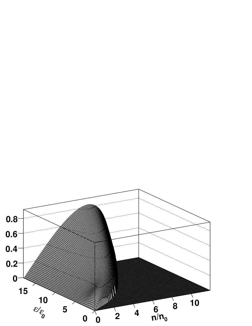
Figure 1: The energy density and net baryon density dependence of ${\cal I}_{30}$ (in units of GeV².fm^-3) for the hadronic part of the equation of state. The energy density and net baryon densities are in units of the ground state densities. $n_{0}$ = 0.16 fm^-3 and $\varepsilon_{0}$ = 0.147 GeV fm^-3.

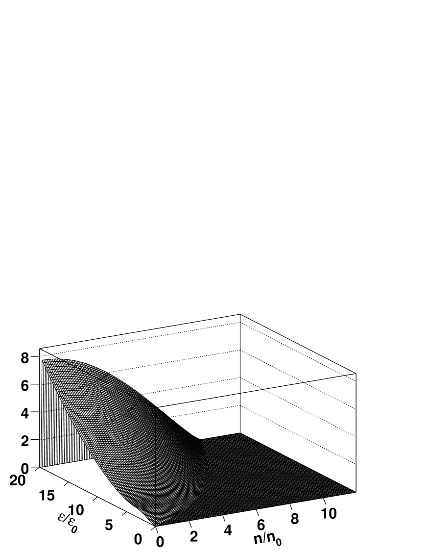
Figure 2: The energy density and net baryon density dependence of ${\cal J}_{50}$ (in units of GeV⁴.fm^-3) for the hadronic part of the equation of state. The energy density and net baryon densities are in units of the ground state densities. $n_{0}$ = 0.16 fm^-3 and $\varepsilon_{0}$ = 0.147 GeV fm^-3.

In Figs. 1 and 2 we show the dependence of the relativistic thermodynamic integrals on this particular equation of state. The results are only for the hadronic phase without the phase transition into the quark gluon plasma. The results of the latter scenario will be explored in full detail somewhere else.

VI Freeze-Out and Particle Spectra

At any space–time point of the many–particle (fluid dynamics) evolution a particle “freezes out” when its interactions with the rest of the system cease. This depends on the mean free path of the particular particle. If the mean free path is small enough such that local thermodynamical equilibrium is established, fluid dynamics is valid. For larger mean free path non-equilibrium effects become increasingly important, and if the mean free path exceeds the system’s dimension, the latter starts to decouple into free-streaming particles. To describe the system’s evolution in the latter two stages in principle requires kinetic theory.

The region where the mean free path is of the order of the system size can be approximated by a hypersurface in space-time Landau ; CF . When a fluid element crosses this hypersurface, particles contained in that element freeze out instantaneously. The freeze-out should be treated in a self-consistent way taking into account the non-equilibrium effects caused by particles leaving the system.

We will consider isothermal freeze-out which corresponds to freeze-out at a constant fluid temperature $T_{f}$. One could also consider freeze-out at a constant center of mass time $t_{f}$. In the later scenario the temperature along the hypersurface is no longer constant.

In the calculations of particle spectra at freeze-out, the distribution of particles that have decoupled from the fluid is determined as follows. The Lorenz-invariant momentum-space distribution of particles crossing a hypersurface $\Sigma$ in Minkowski space is given by CF

$$E{\mbox{d}N\over\mbox{d}^{3}{{\bf p}}}=\int_{\Sigma}\mbox{d}\Sigma_{\mu}p^{\mu}f(x,p)~{},$$ (128)

where $\mbox{d}\Sigma_{\mu}$ is the normal vector on an infinitesimal element of the hypersurface $\Sigma$. $\mbox{d}\Sigma_{\mu}$ is naturally chosen to point outwards with respect to the hotter interior of $\Sigma$ since Eq. (128) is supposed to give the momentum distribution of particles decoupling from the fluid. The distribution function $f(x,p)$ is given by Eq. (29).

The calculations simplifies in the case of longitudinal boost invariance and transverse translation invariance Bj . In this case the on-shell phase space distribution function depends only on the reduced phase space variables $(\tau,\chi,{\bf p}_{\perp})$, where $\tau^{2}=t^{2}-z^{2}$ and $\chi=\eta-y$, in terms of the (longitudinal) particle rapidity $y=\tanh^{-1}(p^{z}/p^{0})$ and the (longitudinal) fluid rapidity $\eta=\tanh^{-1}(z/t)$. The collective flow velocity field, the momentum and the heat flux in this case are given by

$$u^{\mu} = x^{\mu}/\tau=(\cosh\eta,{\bf 0}_{\perp},\sinh\eta)~{},$$ (129)

$$p^{\mu} = (m_{\perp}\cosh y,p_{\perp}\cos\phi_{p},p_{\perp}\sin\phi_{p},m_{\perp}\sinh y)~{},$$ (130)

$$q^{\mu} = ql^{\mu}=q(\sinh\eta,{\bf 0}_{\perp},\cosh\eta)~{},$$ (131)

where $l^{\mu}$ is a space-like 4-vector $l^{\mu}l_{\mu}=-1$ and it is orthogonal to the 4-velocity $l^{\mu}u_{\mu}=0$, $\phi_{p}$ is the angle of particle’s momentum around the $z$-axis and $m_{\perp}=\sqrt{\mbox{\boldmath${p}$}_{\perp}^{2}+m^{2}}$ is the transverse mass which reduces to $p_{\perp}$ for the massless particles. The shear tensor is given by

$$\pi^{\mu\nu}=\begin{pmatrix}\pi_{s}\sinh^{2}\eta&\quad 0&\quad 0&\quad\pi_{s}\cosh\eta\sinh\eta\\ 0&\quad-{\pi_{s}\over 2}&\quad 0&\quad 0\\ 0&\quad 0&\quad-{\pi_{s}\over 2}&\quad 0\\ \pi_{s}\cosh\eta\sinh\eta&\quad 0&\quad 0&\quad\pi_{s}\cosh^{2}\eta\end{pmatrix}~{},$$ (132)

where $\pi_{s}$ is the scalar shear pressure (to distinguish it from the constant $\pi$). In our particular case at freeze-out $\tau=\tau_{f}$, $\Sigma$ is conveniently parameterized by $\Sigma^{\mu}=(\tau_{f}\cosh\eta,{\bf x}_{\perp},\tau_{f}\sinh\eta)$ with $\mbox{d}\Sigma^{\mu}=(\tau_{f}\cosh\eta,{\bf 0}_{\perp},-\tau_{f}\sinh\eta)\mbox{d}\eta\mbox{d}{\bf x}_{\perp}$. Therefore, $\mbox{d}\Sigma^{\mu}p_{\mu}=\tau_{f}m_{\perp}\cosh\chi\mbox{d}\eta\mbox{d}{\bf x}_{\perp}$ and $p^{\mu}u_{\mu}=m_{\perp}\cosh\chi$.

The distribution function however now includes the corrections due to dissipative effects. Now there is the equilibrium part and non-equilibrium part. With the expressions, Eqs. (54)–(56), for $\epsilon(x)$, $\epsilon_{\nu}(x)$ and $\epsilon_{\mu\nu}(x)$ in terms of the dissipative fluxes we can write the deviation function as

$$\phi(x,p)=\left[{\cal A}_{0}-{\cal A}_{1}(p^{\mu}u_{\mu})+\left[4(p^{\mu}u_{\mu})^{2}-m^{2}\right]{\cal A}_{2}\right]\Pi+\left[{\cal B}_{0}-{\cal B}_{1}(p^{\mu}u_{\mu})\right](p^{\mu}q_{\mu})+{\cal C}_{0}p^{\mu}p^{\nu}\pi_{\mu\nu}+\cdot\cdot\cdot~{}.$$ (133)

In our present freeze-out prescription we have

$$p^{\mu}q_{\mu} = qm_{\perp}\sinh\chi~{},$$ (134)

$$p^{\mu}p^{\nu}\pi_{\mu\nu} = \pi_{s}m_{\perp}^{2}\sinh^{2}\chi-{1\over 2}\pi_{s}p_{\perp}^{2}~{},$$ (135)

and the deviation function becomes

$$\phi(x,p) = \left[{\cal A}_{0}-{\cal A}_{1}(m_{\perp}\cosh\chi)+[4(m_{\perp}\cosh\chi)^{2}-m^{2}]{\cal A}_{2}\right]\Pi$$ (136)

$$+\left[{\cal B}_{0}-{\cal B}_{1}(m_{\perp}\cosh\chi)\right](m_{\perp}\sinh\chi)q$$

$$+{\cal C}_{0}\left[m^{2}_{\perp}\sinh^{2}\chi-{1\over 2}p_{\perp}^{2}\right]\pi_{s}~{}.$$

In the freeze-out prescription of a system with longitudinal boost invariance and transverse cylindrical symmetry MR one frequently uses the integrals of the form

$$\chi_{ijmn}^{(1)} = \int_{0}^{2\pi}\mbox{d}\psi\sin^{i}\psi\cos^{j}\psi\int_{0}^{\infty}\mbox{d}\chi\sinh^{m}\chi\cosh^{n}\chi$$ (137)

$$\times{1\over e^{z_{\perp}\cosh\chi-\alpha_{\perp}\cos\psi-\phi}-a}~{},$$

$$\chi_{ijmn}^{(2)} = \int_{0}^{2\pi}\mbox{d}\psi\sin^{i}\psi\cos^{j}\psi\int_{0}^{\infty}\mbox{d}\chi\sinh^{m}\chi\cosh^{n}\chi$$ (138)

$$\times{e^{z_{\perp}\cosh\chi-\alpha_{\perp}\cos\psi-\phi}\over\left[e^{z_{\perp}\cosh\chi-\alpha_{\perp}\cos\psi-\phi}-a\right]^{2}}~{},$$

where $\psi=\phi-\phi_{p}$ is given in terms of the azimuthal angle of the surface element of the fluid $\phi$ and the angle of the particle’s momentum $\phi_{p}$ around $z$, $z_{\perp}=\gamma_{\perp}m_{\perp}/T$ and $\alpha_{\perp}=\gamma_{\perp}v_{\perp}p_{\perp}/T$. The powers in the trigonometric and hyperbolic functions comes from the product of the volume element parameterization in cylindrical coordinates with boost invariance and the distribution function $f(x,p)\equiv f(p_{\mu}u^{\mu},\Pi,p_{\mu}q^{\mu},p_{\mu}p_{\nu}\pi^{\mu\nu})$ as given by Eq. (29). Eq. (137) arises due to the first term of Eq. (29) and this gives the equilibrium (ideal fluid) contribution to the spectra while Eq. (138) arises from the second term of Eq. (29) and it gives non-equilibrium (non-ideal fluid) contribution to the spectra. Expanding the Fermi-Dirac and Bose-Einstein distribution functions in geometric series we can write Eqs. (137) and (138) as

$$\chi_{ijmn}^{(1)} = \sum_{k=1}^{\infty}\left(\mp\right)^{k-1}e^{k\phi}$$ (139)

$$\times\int_{0}^{2\pi}\mbox{d}\psi\sin^{i}\psi\cos^{j}\psi e^{k\alpha_{\perp}\cos\psi}\int_{0}^{\infty}\mbox{d}\chi\sinh^{m}\chi\cosh^{n}\chi e^{-kz_{\perp}\cosh\chi}~{},$$

$$\chi_{ijmn}^{(2)} = \sum_{k=1}^{\infty}\left(\mp\right)^{k-1}ke^{k\phi}$$ (140)

$$\times\int_{0}^{2\pi}\mbox{d}\psi\sin^{i}\psi\cos^{j}\psi e^{k\alpha_{\perp}\cos\psi}\int_{0}^{\infty}\mbox{d}\chi\sinh^{m}\chi\cosh^{n}\chi e^{-kz_{\perp}\cosh\chi}~{},$$

where the upper sign is for fermions and the bottom one is for bosons. Using the integral representation of the modified Bessel functions of the first kind $I_{n}(x)$ and of the second kind $K_{n}(x)$ we can write

$$\chi_{ijmn}^{(1)} = \sum_{k=1}^{\infty}\left(\mp\right)^{k-1}e^{k\phi}i_{ij}(k\alpha_{\perp})k_{mn}(kz_{\perp})~{},$$ (141)

$$\chi_{ijmn}^{(2)} = \sum_{k=1}^{\infty}\left(\mp\right)^{k-1}ke^{k\phi}i_{ij}(k\alpha_{\perp})k_{mn}(kz_{\perp})~{},$$ (142)

where

$$i_{ij} = \sum_{l=0}^{[(1/2)d]}\left(\begin{array}[]{c}\displaystyle{[(1/2)d]}\\ \displaystyle{l}\end{array}\right)(2b+2l-1)!!y^{-b-l}2\pi I_{b+l+h}(y)~{},$$ (145)

$$k_{mn} = \sum_{l=0}^{[(1/2)d]}\left(\begin{array}[]{c}\displaystyle{[(1/2)d]}\\ \displaystyle{l}\end{array}\right)(2b+2l-1)!!y^{-b-l}K_{b+l+h}(y)~{},$$ (148)

and $[p]$ stands for the largest integer not exceeding $p$. In $i_{ij}$, ($d=j$, $b=i/2$, $y=k\alpha_{\perp}$) while in $k_{mn}$, ($d=n$, $b=m/2$, $y=kz_{\perp}$). Furthermore, $h$ is zero or one depending on whether $d$ is even or odd respectively. Note also that for odd powers in $\sin\psi$ the $i_{ij}$ vanishes and similarly for odd powers of $\sinh\chi$ the $k_{mn}$ vanishes.

In the case of pure longitudinal expansion $i=j=0$ and $\alpha_{\perp}=0$. Then $i_{ij}(k\alpha_{\perp})=i_{00}(0)=2\pi$ and $\chi_{ijmn}$ reduces to

$$\chi_{00mn}^{(1)} = 2\pi\sum_{k=1}^{\infty}\left(\mp\right)^{k-1}e^{k\phi}k_{mn}(kz_{\perp})~{},$$ (149)

$$\chi_{00mn}^{(2)} = 2\pi\sum_{k=1}^{\infty}\left(\mp\right)^{k-1}ke^{k\phi}k_{mn}(kz_{\perp})~{}.$$ (150)

The inclusive particle distribution and transverse energy at freeze-out are given by

$${\mbox{d}N(\tau_{f})\over\mbox{d}y\mbox{d}^{2}{{\bf p}_{\perp}}} = \int\tau_{f}\mbox{d}\eta\mbox{d}^{2}{{\bf x}_{\perp}}{m_{\perp}}\cosh\chi\,f(x,p)~{},$$ (151)

$${\mbox{d}{E_{\perp}}\over\mbox{d}y} = \int\mbox{d}^{2}{{\bf p}_{\perp}}{m_{\perp}}{\mbox{d}N(\tau_{f})\over\mbox{d}y\mbox{d}^{2}{{\bf p}_{\perp}}}=\int\tau_{f}\mbox{d}\eta\mbox{d}^{2}{{\bf x}_{\perp}}\int\mbox{d}^{2}{{\bf p}_{\perp}}{m_{\perp}^{2}}\cosh\chi\,f(x,p)~{}.$$ (152)

Using Eq. (29), for the distribution function $f(x,p)$, the particle spectra can be written as

$${\mbox{d}N(\tau_{f})\over\mbox{d}y\mbox{d}^{2}{{\bf p}_{\perp}}}=\int\tau_{f}\mbox{d}\eta\mbox{d}^{2}{{\bf x}_{\perp}}{m_{\perp}}\cosh\chi\left\{f^{{\rm eq}}(x,p)+f^{{\rm eq}}(x,p)\Delta^{{\rm eq}}(x,p)\phi(x,p)\right\}~{},$$ (153)

where

$$f^{{\rm eq}}(x,p)=A_{0}{1\over\mbox{\rm exp}\{m_{\bot}\cosh\chi/T\}-1}~{}.$$ (154)

The first term in the curly brackets of Eq. (153) is the equilibrium contribution to the spectra while the second term is the non-equilibrium contribution to the spectra. Using the expression for $\phi(x,p)$ and the integral representation $\chi_{ijmn}$ the particle distribution becomes

$${\mbox{d}N(\tau_{f})\over\mbox{d}y\mbox{d}^{2}{{\bf p}_{\perp}}} = A_{0}{1\over 2}R_{\perp}^{2}\tau_{f}\times\biggl{\{}\chi_{0001}^{(1)}+\left[({\cal A}_{0}-m^{2}{\cal A}_{2})\chi_{0001}^{(2)}-{\cal A}_{1}{m_{\perp}}\chi_{0002}^{(2)}+4{\cal A}_{2}{m_{\perp}^{2}}\chi_{0003}^{(2)}\right]\Pi$$ (155)

$$+{\cal C}_{0}\left[{m_{\perp}^{2}}\chi_{0021}^{(2)}-{1\over 2}{p_{\perp}^{2}}\chi_{0001}^{(2)}\right]\pi_{s}\biggr{\}}$$

where the first term which involves the $\chi_{ijmn}^{(1)}$ is the equilibrium spectrum and the rest of the terms that involves $\chi_{ijmn}^{(2)}$ represent the non-equilibrium contribution to the spectrum, i.e, they represent the corrections to the particle spectra due to dissipation. For dissipative corrections of particle spectra due to shear viscosity only we find, using Eqs. (137) and (138),

$${\mbox{d}N(\tau_{f})\over\mbox{d}y\mbox{d}^{2}{{\bf p}_{\perp}}}=A_{0}\pi R_{\perp}^{2}\tau_{f}{m_{\perp}}{1\over 4}{\pi_{s}\over\varepsilon+p}K_{1}({z_{\perp}})\biggl{[}{\alpha_{\perp}^{2}}-\frac{1}{2}{z_{\perp}^{2}}\biggl{(}{K_{3}({z_{\perp}})\over K_{1}({z_{\perp}})}-1\biggr{)}\biggr{]}$$ (156)

In the case of a pure (1+1)-dimensional expansion in planar geometry, the transverse dimension enters only as a (constant) transverse area factor $A$. The parametric integration over the hypersurface $\Sigma$ in Eq. (128) is performed by distinguishing space-like parts $\Sigma_{s}$ (with $z$ as integration variable) and time-like parts $\Sigma_{t}$ (with $t$ as integration variable). This yields the total momentum–space distribution

$$\frac{{\rm d}N}{{\rm d}yp_{\bot}{\rm d}p_{\bot}} = 2\pi A\,m_{\bot}\left[\int_{\Sigma_{s}}{\rm d}z~{}[\cosh y-\sinh y(\partial t/\partial z)_{\Sigma}]f(x,p)\right.$$ (157)

$$\left.+\int_{\Sigma_{t}}{\rm d}t~{}[\cosh y(\partial z/\partial t)_{\Sigma}-\sinh y]f(x,p)\right]~{},$$

where $(\partial t/\partial z)_{\Sigma}$ is the (local) slope of the space-like hypersurface element. In the expression for the distribution function Eq. (29) the equilibrium distribution $f^{eq}$ is given by Eq. (154) while $\phi(x,p)$ is given by Eq. (136). Note that in pure (1+1)-dimensional expansion we have only one independent component of heat flux which we take to be $q^{z}=\gamma{\cal Q}^{z}=\gamma q$ and one independent component of shear stress tensor which we take to be $\pi^{zz}=\gamma^{2}\tau^{zz}=\gamma^{2}\pi_{s}$. We simply write $q$ for the local rest frame independent component of heat flux ${\cal Q}^{z}$ and $\pi_{s}$ for the local rest frame independent component of shear stress tensor $\tau^{zz}$. From AMI we know that the other nonvanishing component of heat flux can be written as $q^{0}=q^{z}v_{z}$ and the other nonvanishing components of the shear stress tensor are $\pi^{00}=\pi^{zz}v_{z}^{2}=\pi_{s}\gamma^{2}v_{z}^{2}$, $\pi^{0z}=\pi^{z0}=\pi^{zz}v_{z}=\pi_{s}\gamma^{2}v_{z}$ and $\pi^{xx}=\pi^{yy}=-\pi_{s}/2$.

We now apply Eq. (157) to the isothermal freeze–out scenario. Along the isotherm, $T=T_{f}={\rm constant}$ and only $\eta$ depends on position or time, respectively. The rapidity distribution is obtained by integrating Eq. (157) over transverse momentum. For massless particles,

$$\frac{{\rm d}N}{{\rm d}y} = 2\pi A\left[\int_{\Sigma_{s}}{\rm d}z~{}{\cosh y-\sinh y(\partial t/\partial z)_{\Sigma}\over\cosh^{3}\chi(z)}{\cal F}\right.$$ (158)

$$\left.+\int_{\Sigma_{t}}{\rm d}t~{}{\cosh y(\partial z/\partial t)_{\Sigma}-\sinh y\over\cosh^{3}\chi(t)}{\cal F}\right]~{},$$

where

$${\cal F} = {1\over 4\pi}\left[{\cal I}_{10}+[{\cal J}_{10}{\cal A}_{0}-{\cal J}_{20}{\cal A}_{1}+4{\cal J}_{30}]\Pi+[{\cal B}_{0}{\cal J}_{20}-{\cal B}_{1}{\cal J}_{30}]q\tanh\chi(z)\right.$$ (159)

$$\left.+{\cal C}_{0}{\cal J}_{30}\pi_{s}\left(1-{3\over 2}{1\over\cosh^{2}\chi(z)}\right)\right]~{},$$

and the ${\cal I}_{nk}$ and the ${\cal J}_{nk}$ are given in Appendix C for single particle species. Analogously, the transverse momentum distribution is obtained integrating over $y$,

$$\frac{{\rm d}N}{p_{\bot}{\rm d}p_{\bot}} = 2\pi~{}p_{\bot}~{}\left[\int_{\Sigma_{s}}{\rm d}z~{}\int_{-\infty}^{\infty}{\rm d}y~{}[\cosh y-\sinh y(\partial t/\partial z)_{\Sigma}]{\cal F}\right.$$ (160)

$$\left.+\int_{\Sigma_{t}}{\rm d}t~{}\int_{-\infty}^{\infty}{\rm d}y~{}[\cosh y(\partial z/\partial t)_{\Sigma}-\sinh y]{\cal F}\right]~{},$$

where

$${\cal F} = A_{0}{1\over\mbox{\rm exp}\{(p_{\bot}/T_{f})\cosh\chi(z)\}-a}$$ (161)

$$+A_{0}{\mbox{\rm exp}\{(p_{\bot}/T_{f})\cosh\chi(z)\}\over[\mbox{\rm exp}\{(p_{\bot}/T_{f})\cosh\chi(z)\}-a]^{2}}\phi(x,p)$$

and

$$\phi(x,p) = \left[{\cal A}_{0}-{\cal A}_{1}p_{\perp}\cosh\chi(z)+4p_{\perp}\cosh^{2}\chi(z){\cal A}_{2}\right]\Pi$$ (162)

$$+\left[{\cal B}_{0}-{\cal B}_{1}p_{\perp}\cosh\chi(z)\right]p_{\perp}\sinh\chi(z)~{}q$$

$$+{\cal C}_{0}\left[p^{2}_{\perp}\sinh^{2}\chi(z)-{1\over 2}p_{\perp}^{2}\right]\pi_{s}~{}.$$

In the isochronous freeze-out scenario the hypersurface $\Sigma$ has no time-like part and the second term in Eq. (157) vanishes. Moreover, also the second term in the numerator of the remaining term vanishes due to $\partial t/\partial z=0$ for this particular hypersurface. The temperature along the hypersurface, however, is no longer constant. Thus the rapidity distribution becomes

$$\frac{{\rm d}N}{{\rm d}y}=2\pi^{2}A\int_{-L-t_{f}}^{L+t_{f}}{\rm d}z{\cosh y\over\cosh^{3}\chi(z)}{\cal F}~{},$$ (163)

with ${\cal F}(z)$ given by Eq. (159) with $T_{f}$ now replaced by $T(z)$. The transverse momentum distribution is

$$\frac{{\rm d}N}{p_{\bot}{\rm d}p_{\bot}}=2\pi A~{}p_{\bot}~{}\int_{-L-t_{f}}^{L+t_{f}}{\rm d}z~{}\int_{-\infty}^{\infty}{\rm d}y~{}\cosh y~{}{\cal F}~{}.$$ (164)

where ${\cal F}$ is given by Eq. (161) with the temperature $T_{f}$ now replaced by $T(z)$. The results of this section generalizes that of Ref. BMGR by including non-equilibrium (dissipative) effects in the freeze-out prescription. The most recent applicatio of freeze-out prescription in the presence of shear viscosity corrections has proven to be excellent in describing the spectra of particles produced at RHIC BR .

VII Summary and conclusions

We have presented a microscopic interpretation of dissipative fluid dynamics by means of the 14-moment method (or 14-Field Theory: an effective kinetic theory for relativistic non-equilibrium fluid dynamics). From the relativistic kinetic theory using Grad’s 14 moment method one obtains relativistic causal fluid dynamics which is a field theory of the 14 fields of net charge density–particle flux and stress–energy–momentum. The field equations are based on the conservation laws of net conserved charge, energy-momentum and on a balance of fluxes. The equations satisfies the principle of relativity, entropy principle and the requirement of hyperbolicity (for causality). The resulting field equations contain only bulk viscosity, shear viscosity and heat conductivity as unknown functions. All other coefficients may be calculated from the equilibrium equations of state. The interface between the microscopic and microscopic in the causal dissipative fluid dynamics is effected via the standard transport coefficients. The comparison between the microscopic and the macroscopic descriptions provides more information on the transport properties that govern the relaxation of various dissipative processes.

From the kinetic theory approach the unknown phenomenological coefficients $\zeta,\,\kappa,\,\eta,\,\alpha_{0},\,\alpha_{1},\,\beta_{0},\,\beta_{1},$ and $\beta_{2}$ can now be explicitly identified from the knowledge of the collision term and the equation of state. We conclude that the 14-Field Theory of viscous, heat-conducting fluids is quite explicit - provided we are given the thermal equation of state $p=p(\alpha,\beta)$ -except for he coefficients ${\cal C}_{A}$. These coefficients must be measured or determined from the underlying theory/model which gave the equation of state.

We have also presented the relativistic thermodynamic integrals in a more general formalism and also for different special cases which are relevant for applications to nuclear collisions applications. These integrals are needed for calculating the second-order relaxation coefficients. The results of the later will be presented in detail somewhere.

Appendix A Relativistic Thermodynamic Integrals

In relativistic kinetic theory one frequently encounters the moments of the distribution function describing local and global equilibrium. The $n$th moment is defined by

$$I^{\mu_{1}...\mu_{n}}(x)=\int\mbox{d}w~{}p^{\mu_{1}}...p^{\mu_{n}}f(x,p)~{},$$ (165)

and the corresponding change of the $n$th moment due to variation of $f(x,p)$ is

$$\delta I^{\mu_{1}...\mu_{n}}(x)=\int\mbox{d}w~{}p^{\mu_{1}}...p^{\mu_{n}}\delta y\Delta(x,p)f(x,p)$$ (166)

where $y=\ln(f(x,p)/\Delta(x,p))$. The variations of moments involves the auxiliary moments

$$J^{\mu_{1}...\mu_{n}}(x)=\int\mbox{d}w~{}p^{\mu_{1}}...p^{\mu_{n}}\Delta(x,p)f(x,p)~{}.$$ (167)

These moments can be expanded in terms of symmetrized tensor product of $u^{\mu}$ and the metric tensor $g^{\mu\nu}$. We define for $2k\leq n$, the set of rank $n$ tensors

$$\bigtriangleup^{(2k}u^{n-2k)}\equiv{2^{k}!k!(n-2k)!\over n!}\sum_{\rm permutations}\bigtriangleup^{\mu_{1}\mu_{2}}...\bigtriangleup^{\mu_{2k-1}\mu_{2k}}u^{\mu_{2k+1}}...u^{\mu_{n}}~{},$$ (168)

where $\bigtriangleup^{\mu\nu}$ is the projector $g^{\mu\nu}-u^{\mu}u^{\nu}$. The sum, which runs over all distinct permutations of the tensor indices, has been divided by the total number of those permutations. The number $k$ can take all integer values between zero and the largest integer not exceeding $n/2$. The latter value will be denoted as $[n/2]$. These tensors possesses the orthogonality property

$$\bigtriangleup^{(2k}u^{n-2k)}\bigtriangleup_{(2l}u_{n-2l)}={(2k+1)!(n-2k)!\over n!}\delta_{ql}~{}.$$ (169)

which arises because of all different terms, differing only by the trivial permutations like $\bigtriangleup^{\mu\nu}\rightarrow\bigtriangleup^{\nu\mu}$, $\bigtriangleup^{\mu\alpha}\bigtriangleup^{\nu\beta}\rightarrow\bigtriangleup^{\nu\beta}\bigtriangleup^{\mu\alpha}$, $u^{\mu}u^{\nu}\rightarrow u^{\nu}u^{\mu}$, only $2^{k}k!(2k)!$ terms survived. If these trivial repetitions are lumped together the expansion contains

$$a_{nk}=\left(\begin{array}[]{c}n\\ 2k\end{array}\right)(2k-1)!!$$ (170)

terms. The double factorial notation stands for $(2k-1)!!=1\cdot 3\cdot 5\cdot\cdot\cdot(2k-1)$ for $k=1,2,\cdots$ and the recursion formula $(2k-1)!!=(2k+1)!!/(2k+1)$ extends the definition to negative integer arguments. The moment integrals are then expanded in the form

$$I^{\mu_{1}...\mu_{n}}=\sum^{[n/2]}_{k=0}a_{nk}{\cal I}_{nk}\bigtriangleup^{(2k}u^{n-2k)}~{},~{}~{}~{}~{}~{}J^{\mu_{1}...\mu_{n}}=\sum^{[n/2]}_{k=0}a_{nk}{\cal J}_{nk}\bigtriangleup^{(2k}u^{n-2k)}~{}.$$ (171)

The scalar coefficients ${\cal I}_{nk}$ and ${\cal J}_{nk}$, which depend on the parameters $\alpha$ and $\beta$ are found by contracting both sides of Eqs. (165) and (167) with a tensor of the form (168) and using the orthogonality property (169). The results of such contractions are

$${\cal I}_{nk}(\alpha,\beta) = {A_{0}\over(2k+1)!!}\int_{0}^{\infty}\mbox{d}w\left[p^{\alpha}u_{\alpha}-p^{\alpha}p_{\alpha}\right]^{k}(p^{\mu}u_{\mu})^{n-2k}$$ (172)

$$~{}~{}~{}~{}~{}~{}~{}~{}~{}~{}~{}~{}~{}~{}~{}~{}~{}~{}\times{1\over e^{\beta p^{\nu}u_{\nu}-\alpha}-a}~{},$$

$${\cal J}_{nk}(\alpha,\beta) = {A_{0}\over(2k+1)!!}\int_{0}^{\infty}\mbox{d}w\left[p^{\alpha}u_{\alpha}-p^{\alpha}p_{\alpha}\right]^{k}(p^{\mu}u_{\mu})^{n-2k}$$ (173)

$$~{}~{}~{}~{}~{}~{}~{}~{}~{}~{}~{}~{}~{}~{}~{}~{}~{}~{}\times{e^{\beta p^{\nu}u_{\nu}-\alpha}\over\left[e^{\beta p^{\nu}u_{\nu}-\alpha}-a\right]^{2}}~{}.$$

The above integrals are invariant scalars, therefore they can be evaluated in any frame. We will evaluate them in the local rest frame. In this frame $u^{\mu}=(1,0,0,0)$, so that $p^{\mu}p_{\mu}=p^{2}=m^{2}$ and $p^{\mu}u_{\mu}=p^{0}=\sqrt{\mbox{\boldmath${p}$}^{2}+m^{2}}$. We introduce spherical polar coordinates $\mbox{d}^{3}{\bf p}=p^{2}\,\mbox{d}p\,\mbox{d}\Omega$. Integrating over $\mbox{d}\Omega$ and introducing new variables

$$x={p\over T}~{},~{}~{}~{}~{}~{}z={m\over T}~{},$$ (174)

the above thermodynamic integrals, Eqs. (172) and (173) may be written as

$${\cal I}_{nk}(\phi,z) = {4\pi A_{0}\over(2k+1)!!}T^{n+2}\int_{0}^{\infty}dx\,x^{2(k+1)}\,(x^{2}+z^{2})^{(n-2k-1)/2}$$ (175)

$$~{}~{}~{}~{}~{}~{}~{}~{}~{}~{}~{}~{}~{}~{}~{}~{}~{}~{}~{}~{}\times{1\over e^{\sqrt{x^{2}+z^{2}}-\phi}-a}~{},$$

$${\cal J}_{nk}(\phi,z) = {4\pi A_{0}\over(2k+1)!!}T^{n+2}\int_{0}^{\infty}dx\,x^{2(k+1)}\,(x^{2}+z^{2})^{(n-2k-1)/2}$$

$$~{}~{}~{}~{}~{}~{}~{}~{}~{}~{}~{}~{}~{}~{}~{}~{}~{}~{}~{}~{}\times{e^{\sqrt{x^{2}+z^{2}}-\phi}\,\over\left\{e^{\sqrt{x^{2}+z^{2}}-\phi}-a\right\}^{2}}~{}$$

$$= {1\over\beta}{\cal I}_{n-1,k-1}+{n-2k\over\beta}{\cal I}_{n-1,k}~{}.$$

The second line of Eq. (A) is obtained by partial integration.

Derivatives of ${\cal I}_{nk}(\phi,z)$ and ${\cal J}_{nk}(\phi,z)$, Eqs. (175) and (A) can be expressed in terms of the ${\cal J}_{nk}(\phi,z)$:

$$\mbox{d}{\cal I}_{nk} = {\cal J}_{nk}\mbox{d}\phi-m^{-1}{\cal J}_{n+1,k}\mbox{d}z~{}$$ (177)

$$= {\cal J}_{nk}\mbox{d}\alpha-{\cal J}_{n+1,k}\mbox{d}\beta~{},$$

$$z\,\mbox{d}{\cal J}_{nk} = m\,[{\cal J}_{n-1,k-1}+(n-2k){\cal J}_{n-1,k}]\mbox{d}\phi-[{\cal J}_{n,k-1}+(n+1-2k){\cal J}_{n,k}]\mbox{d}z~{},$$

$$\beta\,\mbox{d}{\cal J}_{nk} = [{\cal J}_{n-1,k-1}+(n-2k){\cal J}_{n-1,k}]\mbox{d}\alpha-[{\cal J}_{n,k-1}+(n+1-2k){\cal J}_{n,k}]\mbox{d}\beta~{}.$$ (178)

For the equation of state $p\equiv p(\varepsilon,n)$ we need the derivative of $p$, $\varepsilon$ and $n$ with respect to ($\phi$, $z$) or with respect to ($\alpha$, $\beta$). From Eq. (177) we have

$$\mbox{d}n \equiv \mbox{d}{\cal I}_{10}={\cal J}_{10}\mbox{d}\alpha-{\cal J}_{20}\mbox{d}\beta,\;\;\;\;\mbox{d}\varepsilon\equiv\mbox{d}{\cal I}_{20}={\cal J}_{20}\mbox{d}\alpha-{\cal J}_{30}\mbox{d}\beta~{},$$ (179)

$$\mbox{d}p \equiv \mbox{d}{\cal I}_{21}={\cal J}_{21}\mbox{d}\alpha-{\cal J}_{31}\mbox{d}\beta,\;\;\;\;\mbox{d}{\cal I}_{31}={\cal J}_{31}\mbox{d}\alpha-{\cal J}_{41}\mbox{d}\beta~{}.$$ (180)

From Eqs. (179) and (180) the differentials of $\alpha(\varepsilon,~{}n)$, $\beta(\varepsilon,~{}n)$, and $p(\varepsilon,~{}n)$ are written as

$$\mbox{d}\alpha = {1\over D_{20}}\left\{{\cal J}_{30}\mbox{d}n-{\cal J}_{20}\mbox{d}\varepsilon\right\},\;\;\;\;\mbox{d}\beta={1\over D_{20}}\left\{{\cal J}_{20}\mbox{d}n-{\cal J}_{10}\mbox{d}\varepsilon\right\}\enspace,$$ (181)

$$\mbox{d}p = {1\over D_{20}}\left\{({\cal J}_{21}{\cal J}_{30}-{\cal J}_{31}{\cal J}_{20})\mbox{d}n-({\cal J}_{21}{\cal J}_{20}-{\cal J}_{31}{\cal J}_{10})\mbox{d}\varepsilon\right\}\enspace.$$ (182)

The fundamental thermodynamic relation together with the first law of thermodynamics can be expressed as

$$nT\mbox{d}(s/n)=\mbox{d}\varepsilon-h\mbox{d}n=({\cal J}_{20}-h{\cal J}_{10})\mbox{d}\alpha-({\cal J}_{30}-h{\cal J}_{20})\mbox{d}\beta~{}.$$ (183)

From Eqs. (179), (180) and (183), the differentials of $\alpha(n,s/n)$ and $\beta(n,s/n)$ can be written as

$$\mbox{d}\alpha = {1\over D_{20}}\left\{({\cal J}_{30}-h{\cal J}_{20})\mbox{d}n-{\cal J}_{20}nT\mbox{d}(s/n)\right\}~{},$$ (184)

$$\mbox{d}\beta = {1\over D_{20}}\left\{({\cal J}_{20}-h{\cal J}_{10})\mbox{d}n-{\cal J}_{10}nT\mbox{d}(s/n)\right\}~{},$$ (185)

and the differentials of $\alpha(\varepsilon,s/n)$ and $\beta(\varepsilon,s/n)$ as

$$\mbox{d}\alpha = {1\over hD_{20}}\left\{({\cal J}_{30}-h{\cal J}_{20})\mbox{d}\varepsilon-{\cal J}_{30}nT\mbox{d}(s/n)\right\}\enspace,$$ (186)

$$\mbox{d}\beta = {1\over hD_{20}}\left\{({\cal J}_{20}-h{\cal J}_{10})\mbox{d}\varepsilon-{\cal J}_{20}nT\mbox{d}(s/n)\right\}\enspace.$$ (187)

Thus from Eqs. (180), (184) and (185) we obtain the expression used in bulk pressure relaxation coefficients, namely

$$\left.{\partial\ln{\cal I}_{31}\over\partial\ln{\cal I}_{10}}\right|_{s/n}=\left.{\partial\ln{\cal J}_{42}\over\partial\ln{\cal I}_{21}}\right|_{s/n}={{\cal J}_{21}\over{\cal J}_{42}}{1\over D_{20}}\left[{\cal J}_{31}({\cal J}_{30}-h{\cal J}_{20})-{\cal J}_{41}({\cal J}_{20}-h{\cal J}_{10})\right]~{}.$$ (188)

From the definitions of specific heats per net conserved charge

$$C_{p}=-\beta\left.{{\partial}(s/n)\over{\partial}\beta}\right|_{p}\,,\,\,C_{V}=-\beta\left.{{\partial}(s/n)\over{\partial}\beta}\right|_{n}\,,\,\,\Gamma=C_{p}/C_{V}~{},$$ (189)

one finds, with the help of Eqs. (179), (180) and (183),

$$C_{p}-C_{V} = \beta^{2}(h{\cal J}_{10}-{\cal J}_{20})^{2}/(n{\cal J}_{10})~{},$$ (190)

$$\Gamma-1 = (h{\cal J}_{10}-{\cal J}_{20})^{2}/D_{20}~{}.$$ (191)

From the definitions of the speed of sound and the compressibilities

$$c_{s}^{2}=\left.{{\partial}p\over{\partial}\varepsilon}\right|_{s/n}=\left.{{\partial}p\over{\partial}\varepsilon}\right|_{n}+{n\over\varepsilon+p}\left.{{\partial}p\over{\partial}n}\right|_{\varepsilon}~{},\;\;\;\alpha_{s}={1\over n}\left.{{\partial}n\over{\partial}p}\right|_{s/n}~{},\;\;\;\kappa_{T}={1\over n}\left.{{\partial}n\over{\partial}p}\right|_{T}~{},$$ (192)

we find, with the help of (179), (180) and (183),

$$c^{2}_{s}={n^{2}\over\beta(\varepsilon+p){\cal J}_{10}}\Gamma,\;\;\;\;\alpha_{s}={\beta{\cal J}_{10}\over n^{2}\Gamma},\;\;\;\;\kappa_{T}={\beta{\cal J}_{10}\over n^{2}}$$ (193)

Thus for a given equation of state, i.e. pressure as a function of two independent state variables, the other thermodynamic quantities can be obtained as partial derivatives of the pressure with respect to $\alpha$ and $\beta$ or to $\phi$ and $z$. This means also that the second order coefficients are also determined from the equation of state.

From the net charge and energy conservation equations (in the particle or Eckart frame)

$$\dot{n}+n\theta=0~{},$$ (194)

$$\dot{\varepsilon}+(\varepsilon+p+\Pi)\theta+(\bigtriangledown_{\mu}q^{\mu}+\pi^{\mu\nu}\bigtriangledown_{\nu}u_{\mu})=0~{},$$ (195)

with the standard notations $\dot{A}\equiv u^{\mu}{\partial}_{\mu}A$ and $\theta\equiv{\partial}_{\mu}u^{\mu}$, we can solve for $\dot{\alpha}$ and $\dot{\beta}$ by simultaneously solving

$${\cal J}_{10}\dot{\alpha}-{\cal J}_{20}\dot{\beta}+{\cal I}_{10}\theta=0~{},$$ (196)

$${\cal J}_{20}\dot{\alpha}-{\cal J}_{30}\dot{\beta}+({\cal I}_{20}+{\cal I}_{21}+\Pi)\theta+(\bigtriangledown_{\mu}q^{\mu}+\pi^{\mu\nu}\bigtriangledown_{\nu}u^{\mu})=0~{},$$ (197)

where we have used Eq. (179). We then find

$$\dot{\beta} = -\frac{{\cal J}_{20}{\cal I}_{10}-{\cal J}_{10}({\cal I}_{20}+{\cal I}_{21}+\Pi)}{D_{20}}\theta+\frac{{\cal J}_{10}(\bigtriangledown_{\mu}q^{\mu}+\pi^{\mu\nu}\bigtriangledown_{\nu}u_{\mu})}{D_{20}}~{},$$ (198)

$$\dot{\alpha} = -\frac{{\cal J}_{30}{\cal I}_{10}-{\cal J}_{20}({\cal I}_{20}+{\cal I}_{21}+\Pi)}{D_{20}}\theta+\frac{{\cal J}_{20}(\bigtriangledown_{\mu}q^{\mu}+\pi^{\mu\nu}\bigtriangledown_{\nu}u_{\mu})}{D_{20}}~{}.$$ (199)

The ${\cal I}_{nk}$ and ${\cal J}_{nk}$ integrals, Eqs. (175) and (A), can be written in terms of the more familiar functions ${\cal K}_{n}(\phi,z),\,{\cal L}_{n+1}(\phi,z)$ defined, for $n\geq 0$, by (cf. IS )

$${\cal K}_{n}(\phi,z) = {1\over(2n-1)!!}{1\over z^{n}}\int_{0}^{\infty}{dx\,x^{2n}\,(x^{2}+z^{2})^{-1/2}\over e^{\sqrt{x^{2}+z^{2}}-\phi}-a}~{},$$ (200)

$${\cal L}_{n+1}(\phi,z) = {1\over(2n-1)!!}{1\over z^{n+1}}\int_{0}^{\infty}{dx\,x^{2n}\over e^{\sqrt{x^{2}+z^{2}}-\phi}-a}~{}.$$ (201)

Partial integration of these functions leads to the following relations

$${{\partial}\over{\partial}\phi}{\cal K}_{n}={\cal L}_{n}~{},~{}~{}~{}~{}~{}{{\partial}\over{\partial}\phi}{\cal L}_{n+1}=-z^{n}{{\partial}\over{\partial}z}\left\{z^{-n}{\cal K}_{n}\right\}={\cal K}_{n-1}+(2n/z){\cal K}_{n}~{}.$$ (202)

In the special case of a Boltzmann gas $(a=0)$, these functions becomes the Bessel functions of the second kind up to a factor of the chemical phase,

$${\cal L}_{n}(\phi,z)={\cal K}_{n}(\phi,z)=e^{\phi}\ K_{n}(z)~{},$$ (203)

where $K_{n}(z)$ are the modified Bessel functions of the second kind.

By making use of the binomial expansion the integrals ${\cal I}_{nk}$ and ${\cal J}_{nk}$, Eqs. (175) and (A), can be expressed in terms of the ${\cal K}_{n}$ and ${\cal L}_{n+1}$, Eqs. (200) and (201). For $n=0,1,...,$ and $k\leq\frac{1}{2}n$, this yields

$${\cal I}_{nk}=4\pi A_{0}m^{n+2}\sum_{l=0}^{\frac{1}{2}n-k}a_{nkl}~{}z^{-(k+l+1)}\left\{\begin{array}[]{ll}{\cal K}_{k+l+1}&\mbox{for even $n$}~{},\\ {\cal L}_{k+l+2}&\mbox{for odd $n$}~{}.\end{array}\right.$$ (204)

and differentiation of these results with respect to $\phi$, (cf. Eqs. (177) and (202)), then gives

$${\cal J}_{nk}=4\pi A_{0}m^{n+2}\sum_{l=0}^{\frac{1}{2}n-k}a_{nkl}~{}z^{-(k+l+1)}\left\{\begin{array}[]{ll}{\cal L}_{k+l+1}&\mbox{for even $n$}\\ {\cal K}_{k+l}+{2(k+l+1)\over z}{\cal K}_{k+l+1}&\mbox{for odd $n$}~{}.\end{array}\right.$$ (205)

The numerical coefficients are

$$a_{nkl}=\frac{(2k+2l+1)!!}{(2k+1)!!}\left(\begin{array}[]{c}\displaystyle{\frac{1}{2}n-k}\\ \displaystyle{l}\end{array}\right)~{}.$$ (206)

Note that in order to calculate the thermodynamic properties of ultra-relativistic (massless) particles using Eqs. (204) and (205) one has to take the limit $m\longrightarrow 0$ (hence $z\longrightarrow 0$) of Eqs. (200) and (201). This is however not necessary if one uses the integral representation Eqs. (175) and (A) since the case for $m=0$ or $z=0$ is included. The integrals ${\cal I}_{nk}$ and ${\cal J}_{nk}$, Eqs. (204) and (205), satisfy the recurrence relations

$${\rm I}_{n+2,k}=m^{2}\,{\rm I}_{nk}+(2k+3){\rm I}_{n+2,k+1}~{}~{}~{}~{}~{}(2k\leq n)~{},$$ (207)

where ${\rm I}_{lm}$ stands for ${\cal I}_{lm}$ or ${\cal J}_{lm}$. This follows from the contractions of Eq. (171).

Appendix B Approximation to thermodynamic integrals

B.1 Nondegenerate gas

If $\phi\leq z$ and $z\neq 0$, the integrals ${\cal I}_{nk}$ and ${\cal J}_{nk}$, Eqs. (175) and (A), may be evaluated SC by making the substitution $x=z\sinh\chi$ expressing the functions $(e^{z\cosh\chi}\pm 1)^{-1}$ as a geometric series in $e^{z\cosh\chi}$ and integrating term by term. The integrals can be written in terms of the Bessel functions with the help of

$${1\over e^{x-\phi}\pm 1}=\sum_{k=1}^{\infty}(\mp)^{k-1}e^{-k(x-\phi)}~{},$$ (208)

$${1\over[e^{x-\phi}\pm 1]^{2}}=\sum_{k=1}^{\infty}(\mp)^{k-1}ke^{-k(x-\phi)}~{},$$ (209)

where the upper sign is for the fermions and the bottom one is for bosons. The integral representation of the Bessel functions of second kind can be written as

$$\int_{0}^{\infty}\mbox{d}\chi\sinh^{2b}\chi\cosh^{d}\chi e^{-y\cosh\chi}=\sum_{r=0}^{[(1/2)d]}\left(\begin{array}[]{c}\displaystyle{[(1/2)d]}\\ \displaystyle{r}\end{array}\right)(2b+2r-1)!!y^{-b-r}K_{b+r+h}(y)~{},$$ (210)

where $h$ is zero or one depending on whether $d$ is even or odd respectively. Then the integrals ${\cal I}_{nk}$ and ${\cal J}_{nk}$, Eqs. (175) and (A), can be written as

$${\cal I}_{nk}^{\pm}(\phi,z) = {4\pi A_{0}\over(2k+1)!!}|\gamma_{Q}|^{i_{q}}\gamma_{p}\sum_{l=1}^{\infty}(\mp 1)^{l-1}\left[e^{l\phi}+(-1)^{n}e^{-l\phi}\right]\sum_{r=0}^{[(1/2)d]}b_{nkr}~{}y^{-b-r}K_{b+r+h}(y)~{},$$ (211)

$${\cal J}_{nk}^{\pm}(\phi,z) = {4\pi A_{0}\over(2k+1)!!}|\gamma_{Q}|^{j_{q}}\gamma_{p}\sum_{l=1}^{\infty}(\mp 1)^{l-1}l\left[e^{l\phi}+(-1)^{n+1}e^{-l\phi}\right]\sum_{r=0}^{[(1/2)d]}b_{nkr}~{}y^{-b-r}K_{b+r+h}(y)~{},$$ (212)

where we have abbreviated

$$b_{nkr}\equiv\left(\begin{array}[]{c}\displaystyle{[(1/2)d]}\\ \displaystyle{r}\end{array}\right)(2b+2r-1)!!~{},~{}~{}~{}~{}~{}b\equiv k+1~{},~{}~{}~{}~{}~{}d\equiv n-2k~{},~{}~{}~{}~{}~{}y\equiv lz~{}.$$ (213)

The superscript notation $\pm$ on the ${\cal I}_{nk}$ and ${\cal J}_{nk}$ indicates that the integrals are evaluated taking into account pair production. The factor $\gamma_{p}$, which is 1 or 1/2 depending on whether the particle is charged or neutral respectively, takes into account the contribution of neutral particles in calculating thermodynamic properties of a gas. $\gamma_{Q}$ is the quantum number for the conserved charge and $i_{q}$ is 1 or 0 depending on whether $n$ is even or odd respectively while $j_{q}$ is 0 or 1 depending on whether $n$ is even or odd respectively.

B.2 Extremely degenerate Fermi gas

This case is relevant to the study of the low temperature region in high energy nuclear collisions and to the study of thermodynamic properties of neutron and quark stars. If $\phi\gg z$, the integrals ${\cal K}_{n}$ and ${\cal L}_{n+1}$, Eqs. (200) and (201), may be expressed in terms of the Chandrasekhar-Sommerfeld asymptotic expansion.

$${\cal K}_{n}(\phi,z) \sim {1\over(2n-1)!!}{1\over z^{n}}\int_{0}^{x_{0}}x^{2n}(x^{2}-z^{2})^{-1/2}\mbox{d}x+2{\pi^{2}\over 12}{1\over(2n-3)!!}{1\over z^{n}}(\phi^{2}-z^{2})^{(2n-3)/2}\phi$$ (214)

$$+2{7\pi^{4}\over 720}{1\over(2n-5)!!}{1\over z^{n}}(\phi^{2}-z^{2})^{(2n-5)/2}\phi\{3+(2n-5)(\phi^{2}-z^{2})^{-1}\phi^{2}\}$$

$$+2{31\pi^{6}\over 30240}{1\over(2n-7)!!}{1\over z^{n}}(\phi^{2}-z^{2})^{(2n-7)/2}\phi$$

$$~{}~{}~{}\times\{15+10(2n-7)(\phi^{2}-z^{2})^{-1}\phi^{2}+(2n-7)(2n-9)(\phi^{2}-z^{2})^{-2}\phi^{4}\}~{},$$

$${\cal L}_{n+1}(\phi,z) \sim {1\over(2n+1)!!}{1\over z^{n+1}}(\phi^{2}-z^{2})^{(2n+1)/2}$$ (215)

$$+2{\pi^{2}\over 12}{1\over(2n-1)!!}{1\over z^{n+1}}(\phi^{2}-z^{2})^{(2n-1)/2}\{1+(2n-1)(\phi^{2}-z^{2})^{-1}\phi^{2}\}$$

$$+2{7\pi^{4}\over 720}{1\over(2n-3)!!}{1\over z^{n+1}}(\phi^{2}-z^{2})^{(2n-3)/2}$$

$$~{}~{}~{}\times\{3+6(2n-3)(\phi^{2}-z^{2})^{-1}\phi^{2}+(2n-3)(2n-5)(\phi^{2}-z^{2})^{-2}\phi^{4}\}$$

$$+2{31\pi^{6}\over 30240}{1\over(2n-5)!!}{1\over z^{n+1}}(\phi^{2}-z^{2})^{(2n-5)/2}$$

$$~{}~{}~{}~{}~{}\times\{15+45(2n-5)(\phi^{2}-z^{2})^{-1}\phi^{2}+15(2n-5)(2n-7)(\phi^{2}-z^{2})^{-2}\phi^{4}$$

$$~{}~{}~{}~{}~{}~{}~{}~{}~{}~{}~{}~{}~{}~{}~{}+(2n-5)(2n-7)(2n-9)(\phi^{2}-z^{2})^{-3}\phi^{6}\}~{},$$

with $x_{0}=\phi$. Changing the variable $x=z\sinh\chi$ one can evaluate the integral

$$R_{n}\equiv{1\over z^{n}}\int_{0}^{x_{0}}x^{2n}(x^{2}-z^{2})^{-1/2}\mbox{d}x=z^{2n}\int_{0}^{\chi_{0}}\sinh^{2n}\chi\mbox{d}\chi~{},$$ (216)

with the help of Eq. (1.412.2) of Ref. GR and the properties of the hyperbolic functions. Here we list the first few expressions for the ${\cal K}_{n}$

$${\cal K}_{0}(\phi,z) \sim \cosh^{-1}(\phi/z)-{\pi^{2}\over 6}{\phi\over(\phi^{2}-z^{2})^{3/2}}-{7\pi^{4}\over 120}{\phi(2\phi^{2}+3z^{2})\over(\phi^{2}-z^{2})^{7/2}}$$ (217)

$$-{31\pi^{6}\over 1008}{\phi(8\phi^{4}+40\phi^{2}z^{2}+15z^{4})\over(\phi^{2}-z^{2})^{11/2}}~{},$$

$$z{\cal K}_{1}(\phi,z) \sim -{1\over 2}z^{2}\cosh^{-1}(\phi/z)+{1\over 2}\phi(\phi^{2}-z^{2})^{1/2}+{\pi^{2}\over 6}{\phi\over(\phi^{2}-z^{2})^{1/2}}+{7\pi^{4}\over 120}{\phi z^{2}\over(\phi^{2}-z^{2})^{5/2}}$$ (218)

$$+{31\pi^{6}\over 1008}{\phi z^{2}(4\phi^{4}+3z^{2})\over(\phi^{2}-z^{2})^{9/2}}~{},$$

$$z^{2}{\cal K}_{2}(\phi,z) \sim {1\over 8}z^{4}\cosh^{-1}(\phi/z)+{1\over 24}\phi(\phi^{2}-z^{2})^{1/2}(2\phi^{2}-5z^{2})+{\pi^{2}\over 6}\phi(\phi^{2}-z^{2})^{1/2}$$ (219)

$$+{7\pi^{4}\over 360}{\phi(2\phi^{2}-3z^{2})\over(\phi^{2}-z^{2})^{3/2}}-{31\pi^{6}\over 1008}{\phi z^{4}\over(\phi^{2}-z^{2})^{7/2}}~{},$$

$$z^{3}{\cal K}_{3}(\phi,z) \sim -{1\over 48}z^{6}\cosh^{-1}(\phi/z)+{1\over 720}\phi(\phi^{2}-z^{2})^{1/2}(8\phi^{4}-26\phi^{2}z^{2}+3z^{4})+{\pi^{2}\over 18}\phi(\phi^{2}-z^{2})^{3/2}$$ (220)

$$+{7\pi^{4}\over 360}{\phi(4\phi^{2}-3z^{2})\over(\phi^{2}-z^{2})^{1/2}}+{31\pi^{6}\over 15120}{\phi(8\phi^{4}-20\phi^{2}z^{2}+15z^{4})\over(\phi^{2}-z^{2})^{5/2}}~{},$$

and for the ${\cal L}_{n+1}$

$$z{\cal L}_{1}(\phi,z) \sim (\phi^{2}-z^{2})^{1/2}-{\pi^{2}\over 6}{z^{2}\over(\phi^{2}-z^{2})^{3/2}}-{7\pi^{4}\over 120}{z^{2}(4\phi^{2}+z^{2})\over(\phi^{2}-z^{2})^{7/2}}$$ (221)

$$-{31\pi^{6}\over 336}{z^{2}(8\phi^{4}+12\phi^{2}z^{2}+z^{4})\over(\phi^{2}-z^{2})^{11/2}}~{},$$

$$z^{2}{\cal L}_{2}(\phi,z) \sim {1\over 3}(\phi^{2}-z^{2})^{3/2}+{\pi^{2}\over 6}{(2\phi^{2}-z^{2})\over(\phi^{2}-z^{2})^{1/2}}+{7\pi^{4}\over 120}{z^{4}\over(\phi^{2}-z^{2})^{5/2}}$$ (222)

$$+{31\pi^{6}\over 1008}{z^{4}(6\phi^{2}+z^{2})\over(\phi^{2}-z^{2})^{9/2}}~{},$$

$$z^{3}{\cal L}_{3}(\phi,z) \sim {1\over 15}(\phi^{2}-z^{2})^{5/2}+{\pi^{2}\over 18}(\phi^{2}-z^{2})^{1/2}(4\phi^{2}-z^{2})+{7\pi^{4}\over 360}{(8\phi^{4}+3z^{4})\over(\phi^{2}-z^{2})^{3/2}}$$ (223)

$$-{31\pi^{6}\over 1008}{z^{6}\over(\phi^{2}-z^{2})^{7/2}}~{},$$

that are needed for the calculation of the ${\cal I}_{nk}$ and ${\cal J}_{nk}$ used in the text.

For a massless Fermi gas the same calculation can be performed for the ${\cal I}_{nk}$ and ${\cal J}_{nk}$ directly using Eqs. (175) and (A)) to give

$${\cal I}_{nk} = {4\pi A_{0}\over(2k+1)!!}T^{n+2}\Biggl{[}{\phi^{n+2}\over n+2}$$

$$+2(n+1)!\left({\pi^{2}\over 12}{\phi^{n}\over n!}+{7\pi^{4}\over 720}{\phi^{n-2}\over(n-2)!}+{31\pi^{6}\over 30240}{\phi^{n-4}\over(n-4)!}+\cdots\right)\Biggr{]}~{},$$

$${\cal J}_{nk} = {4\pi A_{0}\over(2k+1)!!}T^{n+2}(n+1)\Biggl{[}{\phi^{n+1}\over n+1}$$ (225)

$$+2n!\left({\pi^{2}\over 12}{\phi^{n-1}\over(n-1)!}+{7\pi^{4}\over 720}{\phi^{n-3}\over(n-3)!}+{31\pi^{6}\over 30240}{\phi^{n-5}\over(n-5)!}+\cdots\right)\Biggr{]}~{}.$$

B.3 Transition region

The representation of the relativistic thermodynamic integrals as series of modified Bessel functions is useful for computation in the non-degenerate case and the representation in the degenerate region gets better for $\phi$ much greater than $z$. A method suitable for the transition region $\phi\sim z$ is needed for computing the values of the integrals in this region and for numerical checking of known results.

The method adopted for the transition region is based on making the substitution $x=t(2z+t^{2})^{1/2}$ in the integrals. The integrals Eqs. (175) and (A) becomes

$${\cal I}_{nk} = {4\pi A_{0}\over(2k+1)!!}T^{n+2}~{}2\int_{0}^{\infty}{t^{2(k+1)}(z+t^{2})^{n-2k}(2z+t^{2})^{k+1/2}dt\over e^{t^{2}+z-\phi}-a}$$ (226)

$${\cal J}_{nk} = {4\pi A_{0}\over(2k+1)!!}T^{n+2}~{}2\int_{0}^{\infty}{t^{2(k+1)}(z+t^{2})^{n-2k}(2z+t^{2})^{k+1/2}dt\over[e^{t^{2}+z-\phi}-a]^{2}}$$ (227)

while the function ${\cal K}_{n}$ and ${\cal L}_{n+1}$, Eqs. (200) and (201) are written as

$${\cal K}_{n} = {1\over(2n-1)!!}{1\over z^{n}}~{}2\int_{0}^{\infty}{t^{2n}(2z+t^{2})^{n-1/2}dt\over e^{t^{2}+z-\phi}-a}$$ (228)

$${\cal L}_{n+1} = {1\over(2n-1)!!}{1\over z^{n}}~{}2\int_{0}^{\infty}{t^{2n}(z+t^{2})(2z+t^{2})^{n-1/2}dt\over e^{t^{2}+z-\phi}-a}$$ (229)

Appendix C Ultrarelativistic Thermodynamic Integrals

C.1 Single particle densities for massless particles

We want to study the thermodynamic properties of an ultrarelativistic gas. Ultrarelativistic particles are characterized by vanishing rest mass. We start by looking at the single particle densities. For ultra-relativistic or massless particles, $z=m/T=0$, the moment integrals, Eqs. (175) and (A) take the simple forms

$${\cal I}_{nk} = {4\pi A_{0}\over(2k+1)!!}T^{n+2}\int_{0}^{\infty}dx\,x^{n+1}{1\over e^{x-\phi}-a}~{},$$ (230)

$${\cal J}_{nk} = {4\pi A_{0}\over(2k+1)!!}T^{n+2}\int_{0}^{\infty}dx\,x^{n+1}{e^{x-\phi}\over\left[e^{x-\phi}-a\right]^{2}}~{}.$$ (231)

For the fermions, when the equilibrium quantities are characterized by $\phi\simeq 0$, we can expand the the integrals in powers of $\phi$. We have

$${\cal I}_{nk} = {4\pi A_{0}\over(2k+1)!!}T^{n+2}\int_{0}^{\infty}dx\,x^{n+1}$$ (232)

$$\times\left[{1\over e^{x-\phi}+1}+\phi{e^{x-\phi}\over\left[e^{x-\phi}+1\right]^{2}}+{1\over 2}\phi^{2}(n+1){x^{n}\over x^{n+1}}{e^{x-\phi}\over\left[e^{x-\phi}+1\right]^{2}}\right]+\cdots~{},$$

$${\cal J}_{nk} = {4\pi A_{0}\over(2k+1)!!}T^{n+2}(n+1)\int_{0}^{\infty}dx\,x^{n}$$ (233)

$$\times\left[{1\over e^{x-\phi}+1}+\phi{e^{x-\phi}\over\left[e^{x-\phi}+1\right]^{2}}+{1\over 2}\phi^{2}n{x^{n-1}\over x^{n}}{e^{x-\phi}\over\left[e^{x-\phi}+1\right]^{2}}\right]+\cdots~{},$$

With the help of (cf. LL2 )

$$\int_{0}^{\infty}\mbox{d}x\,x^{n+1}{1\over e^{x}+1} = (1-2^{-(n+1)})\Gamma(n+2)\zeta(n+2)~{},$$ (234)

$$\int_{0}^{\infty}\mbox{d}x\,x^{n+1}{e^{x}\over(e^{x}+1)^{2}} = (1-2^{-n})\Gamma(n+2)\zeta(n+1)~{},$$ (235)

where $\Gamma(x)$ is the Gamma function and $\zeta(x)$ is the Riemann’s zeta function, (Note that the $\zeta$ function with even argument is analytically known), we get, for a gas of quarks,

$${\cal I}_{nk} = {g_{Q}\over 2\pi^{2}}{1\over(2k+1)!!}T^{n+2}\Biggl{[}(1-2^{-(n+1)})\Gamma(n+2)\zeta(n+2)$$ (236)

$$+\phi(1-2^{-n})\Gamma(n+2)\zeta(n+1)+{1\over 2}\phi^{2}(n+1)(1-2^{-(n-1)})\Gamma(n+1)\zeta(n)\Biggr{]}+\cdots~{},$$

$${\cal J}_{nk} = {g_{Q}\over 2\pi^{2}}{1\over(2k+1)!!}T^{n+2}(n+1)\Biggl{[}(1-2^{-n})\Gamma(n+1)\zeta(n+1)$$ (237)

$$+\phi(1-2^{-(n-1)})\Gamma(n+1)\zeta(n)+{1\over 2}\phi^{2}n(1-2^{-(n-2)})\Gamma(n)\zeta(n-1)\Biggr{]}+\cdots~{},$$

with $g_{Q}$ the quark degeneracy. For the antiquarks we replace $\phi$ by $-\phi$. For gluons, $\phi=0$, and with the help of (cf. LL2 )

$$\int_{0}^{\infty}\mbox{d}x\,x^{n+1}{1\over e^{x}-1} = \Gamma(n+2)\zeta(n+2)~{},$$ (238)

$$\int_{0}^{\infty}\mbox{d}x\,x^{n+1}{e^{x}\over(e^{x}-1)^{2}} = \Gamma(n+2)\zeta(n+1)~{},$$ (239)

we have

$${\cal I}_{nk} = {g_{G}\over 2\pi^{2}}{1\over(2k+1)!!}T^{n+2}\Gamma(n+2)\zeta(n+2)~{},$$ (240)

$${\cal J}_{nk} = {g_{G}\over 2\pi^{2}}{1\over(2k+1)!!}T^{n+2}\Gamma(n+2)\zeta(n+1)~{},$$ (241)

with $g_{G}$ the gluon degeneracy.

As an example, the number density, energy density and pressure of quarks are given by

$$n_{q} = {\cal I}_{10}={g_{Q}\over 2\pi^{2}}T^{3}\left[{3\over 2}\zeta(3)+\phi{\pi^{2}\over 6}\right]~{},$$ (242)

$$\varepsilon_{q} = {\cal I}_{20}={g_{Q}\over 2\pi^{2}}T^{4}\left[{7\over 4}{\pi^{4}\over 30}+\phi{9\over 2}\zeta(3)+{1\over 2}\phi^{2}{\pi^{2}\over 2}\right]~{},$$ (243)

$$p_{q} = {\cal I}_{21}={1\over 3}{\cal I}_{20}~{}.$$ (244)

and for the antiquarks one replaces $\phi$ by $-\phi$. Similarly, the number density, energy density and pressure of gluons are calculated using the boson integrals to give

$$n_{g}={\cal I}_{10}=g_{G}{\zeta(3)\over\pi^{2}}T^{3},\;\;\;\;\varepsilon_{g}={\cal I}_{20}=g_{G}{\pi^{2}\over 30}T^{4},\;\;\;\;p_{g}={1\over 3}\varepsilon_{g}={\cal I}_{21}={1\over 3}{\cal I}_{20}~{}.$$ (245)

We can also calculate the relaxation and coupling coefficients for the quarks and gluons. For $\phi=0$ one can immediately check that for massless particles the quantity $\Omega$ given by Eq. (61) that comes in the relaxation and coupling coefficients for bulk pressure vanishes identically. Thus those coefficients then diverges. That is, $\Omega\Longrightarrow 0\,,\,\,\,\alpha_{0}\Longrightarrow\infty\,,\,\,\,\beta_{0}\Longrightarrow\infty$. This have the consequence that the bulk viscosity itself has to go to zero. For the shear tensor relaxation coefficients, we have for the quarks and gluons respectively

$$\beta_{2}^{q} = {3\over 4}\times 31\times{8\over 15^{2}}{\zeta(6)\zeta(4)\over\zeta(5)\zeta(5)}\,{1\over p}~{},$$ (246)

$$\beta_{2}^{g} = {3\over 4}{\zeta(6)\zeta(4)\over\zeta(5)\zeta(5)}\,{1\over p}~{}.$$ (247)

For a classical Boltzmann gas in the ultra-relativistic limit $(z\ll 1)$ one gets the following expression for the shear relaxation coefficient

$$\beta_{2}={3\over 4}p^{-1}~{}.$$ (248)

C.2 A system of massless particles and antiparticles

We now consider a gas of particles and antiparticles. For ultrarelativistic Bose gas the chemical potential is zero and the contribution of bosons to the thermodynamic properties of the gas is given by Eqs. (240) (with $n$ even, since for odd values of $n$ there are cancellations, e.g., net baryon number vanishes) and (241) (with $n$ odd, since for even values of $n$ there are cancellations). The same argument goes for the ultrarelativistic Fermi gas with vanishing chemical potential. But here we are considering a gas at finite chemical potential. For ultrarelativistic or massless particles, $z=m/T=0$, the moment integrals, Eqs. (175) and (A) takes the simple forms

$${\cal I}_{nk}^{\pm} = {4\pi A_{0}\over(2k+1)!!}T^{n+2}\int_{0}^{\infty}dx\,x^{n+1}\left\{{1\over e^{x-\phi}+1}+(-1)^{n}{1\over e^{x+\phi}+1}\right\}~{},$$ (249)

$${\cal J}_{nk}^{\pm} = {4\pi A_{0}\over(2k+1)!!}T^{n+2}\int_{0}^{\infty}dx\,x^{n+1}\left\{{e^{x-\phi}\over\left[e^{x-\phi}+1\right]^{2}}+(-1)^{n+1}{e^{x+\phi}\over\left[e^{x+\phi}+1\right]^{2}}\right\}~{}.$$ (250)

These integrals can be evaluated by analytical means. We substitute $y^{-}=x-\phi$ in the first term and $y^{+}=x+\phi$ in the second term and then write the integrals so that we can integrate from 0 to $\infty$. Then we have

$${\cal I}_{nk}^{\pm} = {4\pi A_{0}\over(2k+1)!!}T^{n+2}\Biggl{[}\int_{0}^{\infty}dy^{+}\,{(y^{+}+\phi)^{n+1}\over e^{y^{+}}+1}+(-1)^{n}\int_{0}^{\infty}dy^{-}\,{(y^{-}-\phi)^{n+1}\over e^{y^{-}}+1}$$ (251)

$$+\int_{-\phi}^{0}dy^{+}\,{(y^{+}+\phi)^{n+1}\over e^{y^{+}}+1}-(-1)^{n}\int_{0}^{\phi}dy^{-}\,{(y^{-}-\phi)^{n+1}\over e^{y^{-}}+1}\Biggr{]}~{},$$

$${\cal J}_{nk}^{\pm} = {4\pi A_{0}\over(2k+1)!!}T^{n+2}(n+1)\Biggl{[}\int_{0}^{\infty}dy^{+}\,{(y^{+}+\phi)^{n}\over e^{y^{+}}+1}+(-1)^{n+1}\int_{0}^{\infty}dy^{-}\,{(y^{-}-\phi)^{n}\over e^{y^{-}}+1}$$ (252)

$$+\int_{-\phi}^{0}dy^{+}\,{(y^{+}+\phi)^{n}\over e^{y^{+}}+1}-(-1)^{n+1}\int_{0}^{\phi}dy^{-}\,{(y^{-}-\phi)^{n}\over e^{y^{-}}+1}\Biggr{]}~{}.$$

For ${\cal J}_{nk}$ we first perform partial integration. The first two integrals can be directly combined and the last two after the substitution $y^{-}=-y^{+}$. We then have

$${\cal I}_{nk}^{\pm} = {4\pi A_{0}\over(2k+1)!!}T^{n+2}\left[\int_{0}^{\infty}dx\,{(x+\phi)^{n+1}+(-1)^{n}(x-\phi)^{n+1}\over e^{x}+1}+\int_{0}^{\phi}dz\,z^{n+1}\right]~{},$$ (253)

$${\cal J}_{nk}^{\pm} = {4\pi A_{0}\over(2k+1)!!}T^{n+2}(n+1)\left[\int_{0}^{\infty}dx\,{(x+\phi)^{n}+(-1)^{n+1}(x-\phi)^{n}\over e^{x}+1}+\int_{0}^{\phi}dz\,z^{n}\right]~{}.$$ (254)

In the last two integrals we noted that $(e^{x}+1)^{-1}+(e^{-x}+1)^{-1}=1$ and we have substituted $z=x+\phi$. The two power functions in the numerator are then expanded according to the binomial expansion. All terms of even $j$ drops out:

$${\cal I}_{nk}^{\pm} = {4\pi A_{0}\over(2k+1)!!}T^{n+2}$$ (257)

$$\times\left[2\sum_{j=1,3,5,\cdots\leq(n+1)}\left(\begin{array}[]{c}\displaystyle{n+1}\\ \displaystyle{j}\end{array}\right)\phi^{n+1-j}\int_{0}^{\infty}dx\,{x^{j}\over e^{x}+1}+\int_{0}^{\phi}dz\,z^{n+1}\right]~{},$$

$${\cal J}_{nk}^{\pm} = {4\pi A_{0}\over(2k+1)!!}T^{n+2}$$ (260)

$$\times(n+1)\left[2\sum_{j=1,3,5,\cdots\leq n}\left(\begin{array}[]{c}\displaystyle{n}\\ \displaystyle{j}\end{array}\right)\phi^{n-j}\int_{0}^{\infty}dx\,{x^{j}\over e^{x}+1}+\int_{0}^{\phi}dz\,z^{n}\right]~{}.$$

The above integrals can be brought to their final analytic form by making use of

$$\int_{0}^{\infty}dx\,{x^{j}\over e^{x}+1}=\Gamma(j+1)\zeta(j+1)\left(1-{1\over 2^{j}}\right)~{}.$$ (261)

Thus we finally have

$${\cal I}_{nk}^{\pm} = {4\pi A_{0}\over(2k+1)!!}T^{n+2}$$ (264)

$$\times\left[2\sum_{j=1,3,5,\cdots\leq(n+1)}\left(\begin{array}[]{c}\displaystyle{n+1}\\ \displaystyle{j}\end{array}\right)\phi^{n+1-j}\Gamma(j+1)\zeta(j+1)\left(1-{1\over 2^{j}}\right)+{\phi^{n+2}\over n+2}\right]$$

$${\cal J}_{nk}^{\pm} = {4\pi A_{0}\over(2k+1)!!}T^{n+2}$$ (267)

$$\times(n+1)\left[2\sum_{j=1,3,5,\cdots\leq n}\left(\begin{array}[]{c}\displaystyle{n}\\ \displaystyle{j}\end{array}\right)\phi^{n-j}\Gamma(j+1)\zeta(j+1)\left(1-{1\over 2^{j}}\right)+{\phi^{n+1}\over n+1}\right]$$

For the total particle number densities or single particle species densities separately one can no longer use the above formulation. One then uses the results from the previous section.

To this end we give here the results of the ultrarelativistic thermodynamic integrals ${\cal I}^{\pm}_{nk}$ and ${\cal J}^{\pm}_{nk}$ for QGP. We present only those that are used in the text. We treat quarks and gluons as ultrarelativistic Fermi or Bose gases, respectively. Then from Eqs. (264) and (267) we have , for a gas of quarks and gluons,

$${\cal I}_{10}^{\pm} = {g_{Q}\over 6}T^{3}\left[\phi+{\phi^{3}\over\pi^{2}}\right]~{},$$ (268)

$${\cal I}_{20}^{\pm} = T^{4}\left[\left(g_{G}+{7\over 4}g_{Q}\right){\pi^{2}\over 30}+g_{Q}\left({\phi^{2}\over 4}+{\phi^{4}\over 8\pi^{2}}\right)\right],\;\;\;\;{\cal I}_{21}^{\pm}={I_{20}^{\pm}\over 3}~{},$$ (269)

$${\cal I}_{30}^{\pm} = g_{Q}T^{5}\left[{7\pi^{2}\over 30}\phi+{\phi^{3}\over 3}+{\phi^{5}\over 10\pi^{2}}\right],\;\;\;\;{\cal I}_{31}^{\pm}={{\cal I}_{30}^{\pm}\over 3}~{},$$ (270)

$${\cal I}_{40}^{\pm} = T^{6}\left[\left(g_{G}+{31\over 16}g_{Q}\right){4\pi^{4}\over 3\times 21}+{g_{Q}\over 12}\left(7\pi^{2}\phi^{2}+5\phi^{4}+{\phi^{6}\over\pi^{2}}\right)\right]~{},$$ (271)

$${\cal I}_{41}^{\pm} = {{\cal I}_{40}\over 3},\;\;\;\;{\cal I}_{42}^{\pm}={{\cal I}_{40}^{\pm}\over 15}~{},$$ (272)

$${\cal J}_{10}^{\pm} = {1\over 2}T^{3}\left[{1\over 3}(g_{G}+g_{Q})+{g_{Q}\over\pi^{2}}\phi^{2}\right]~{},$$ (273)

$${\cal J}_{20}^{\pm} = {g_{Q}\over 2}T^{4}\left[\phi+{\phi^{3}\over\pi^{2}}\right],\;\;\;\;{\cal J}_{21}^{\pm}={{\cal J}_{20}^{\pm}\over 3}~{},$$ (274)

$${\cal J}_{30}^{\pm} = T^{5}\left[\left(g_{G}+{7\over 4}g_{Q}\right){2\pi^{2}\over 15}+g_{Q}\left(\phi^{2}+{\phi^{4}\over 2\pi^{2}}\right)\right],\;\;\;\;{\cal J}_{31}^{\pm}={{\cal J}_{30}^{\pm}\over 3}~{},$$ (275)

$${\cal J}_{40}^{\pm} = g_{Q}T^{6}\left[{7\pi^{2}\over 6}\phi+{5\over 3}\phi^{3}+{\phi^{5}\over 2\pi^{2}}\right],\;\;\;\;{\cal J}_{41}^{\pm}={{\cal J}_{40}\over 3},\;\;\;\;{\cal J}_{42}^{\pm}={{\cal J}_{40}^{\pm}\over 15}~{},$$ (276)

$${\cal J}_{50}^{\pm} = T^{7}\left[\left(g_{G}+{31\over 16}g_{Q}\right){8\pi^{4}\over 21}+{g_{Q}\over 2}\left(7\pi^{2}\phi^{2}+5\phi^{4}+{\phi^{6}\over\pi^{2}}\right)\right]~{},$$ (277)

$${\cal J}_{51}^{\pm} = {{\cal J}_{50}^{\pm}\over 3},\;\;\;\;{\cal J}_{52}^{\pm}={{\cal J}_{50}^{\pm}\over 15}~{},$$ (278)

where $g_{G}=N_{s}(N_{c}^{2}-1)$ and $g_{Q}=N_{s}N_{c}N_{f}$, (with $N_{s}$ the number of spin projections, $N_{c}$ the number of color charges and $N_{f}$ the number of quark flavours) are the quark and gluon degeneracies respectively. Note that the net baryon charge is $n={\cal I}^{\pm}_{10}$ while the total energy density and the total pressure are given by $\varepsilon={\cal I}^{\pm}_{20}$ and $p={\cal I}^{\pm}_{21}$.

Appendix D Relativistic thermodynamic integrals at zero temperature, T=0

At $T=0$ the mean occupation number is in good approximation described by the step function and the relativistic thermodynamic integrals Eqs. (172) and (173) becomes

$${\cal I}_{nk} = {4\pi A_{0}\over(2k+1)!!}\int_{0}^{p_{f}}(p^{2}+m^{2})^{(n-2k-1)/2}p^{2(k+1)}\mbox{d}p$$ (279)

$${\cal J}_{nk} = 0$$ (280)

The ${\cal J}_{nk}$ integrals vanishes at $T=0$ because they are the product of temperature and the delta function or the ${\cal I}_{nk}$ integrals. To calculate the integrals Eq. (279) we make the substitution $p=m\sinh\chi$. Then we have $\mbox{d}p=m\cosh\chi\,\mbox{d}\chi$. If we set $p_{f}=m\sinh\chi_{f}$ then the integrals Eq. (279) becomes

$${\cal I}_{nk}={4\pi A_{0}\over(2k+1)!!}m^{n+2}\int_{0}^{\chi_{f}}\cosh^{n-2k}\chi\sinh^{2(k+1)}\chi\,\mbox{d}\chi$$ (281)

For massless particles Eq. (279) becomes

$${\cal I}_{nk} = {4\pi A_{0}\over(2k+1)!!}\int_{0}^{p_{f}}p^{n+1}\mbox{d}p$$ (282)

$$= {4\pi A_{0}\over(2k+1)!!}{p_{f}^{n+2}\over n+2}$$

The integrals Eq. (281) are evaluated with the help of Eq. (2.413) of Ref. GR and the properties of the hyperbolic functions. Here we list the results which are used in the text:

$${\cal I}_{10} = 4\pi A_{0}m^{3}\left[{1\over 3}\sinh^{3}\chi_{f}\right]$$ (283)

$${\cal I}_{20} = 4\pi A_{0}m^{4}\left[-{\chi_{f}\over 8}+{1\over 32}\sinh 4\chi_{f}\right]$$ (284)

$${\cal I}_{21} = {4\pi A_{0}\over 3}m^{4}\left[{3\over 8}\chi_{f}-{3\over 8}\sinh\chi_{f}\cosh\chi_{f}+{1\over 4}\sinh^{3}\chi_{f}\cosh\chi_{f}\right]$$ (285)

$${\cal I}_{30} = 4\pi A_{0}m^{5}\left[{1\over 5}\left(\cosh^{2}\chi_{f}+{2\over 3}\right)\sinh^{3}\chi_{f}\right]$$ (286)

$${\cal I}_{31} = {4\pi A_{0}\over 3}m^{5}\left[{1\over 5}\sinh^{5}\chi_{f}\right]$$ (287)

The Fermi momentum $p_{f}$ can be determined from the net charge density

$$p_{f}=\left({3\over 4\pi A_{0}}{\cal I}_{10}\right)^{1/3}\\$$ (288)

from which $\chi_{f}=\sinh^{-1}\left(p_{f}/m\right)$