Global study of the spectroscopic properties of the first $2^{+}$ state in even-even nuclei

Abstract

We discuss the systematics of the $2^{+}$ excitation energy and the transition probability from this $2^{+}$ to the ground state for most of the even-even nuclei, from ¹⁶O up to the actinides, for which data are available. To that aim we calculate their correlated $J=0$ ground state and $J=2$ first excited state by means of the angular-momentum and particle-number projected generator coordinate method, using the axial mass quadrupole moment as the generator coordinate and self-consistent mean-field states only restricted by axial, parity, and time-reversal symmetries. The calculation, which is an extension of a previous systematic calculation of correlations in the ground state, is performed within the framework of a non-relativistic self-consistent mean-field model using the same Skyrme interaction SLy4 and a density-dependent pairing force to generate the mean-field configurations and mix them. To separate the effects due to angular-momentum projection and those related to configuration mixing, the comparison with the experimental data is performed for the full calculation and also by taking a single configuration for each angular momentum, chosen to minimize the projected energy. The theoretical energies span more than 2 orders of magnitude, ranging below 100 keV in deformed actinide nuclei to a few MeV in doubly-magic nuclei. Both approaches systematically overpredict the experiment excitation energy, by an average factor of about 1.5. The dispersion around the average is significantly better in the configuration mixing approach compared to the single-configuration results, showing the improvement brought by the inclusion of a dispersion on the quadrupole moment in the collective wave function. Both methods do much better for the quadrupole properties; using the configuration mixing approach the mean error on the experimental $B(E2)$ values is only 50$\%$. We discuss possible improvements of the theory that could be made by introducing other constraining fields.

I Introduction

Self-consistent mean-field methods (SCMF) are the only computationally tractable methods which can be applied to medium and heavy nuclei and have a well-justified foundation in many-body theory RMP . Recently there has been considerable progresses in using these methods to compute nuclear mass tables doba . One of the appealing features of the SCMF is that the properties of all nuclei are derived from a fixed energy density functional that depends on a small number of universal parameters, and can be used for the entire chart of nuclei. The Skyrme family of functionals which is used in the present study, depends on about 10 parameters for the particle-hole interaction with 2-3 extra parameters for the pairing interaction.

In a previous study Ben05a ; Ben06 , we have used an extended SCMF theory to calculate the ground state binding energies of the about $600$ even-even nuclei whose masses are known experimentally. In particular, two extensions were introduced to treat correlation effects going beyond a mean field approach. The first is a projection of the SCMF wave functions to restore symmetries broken by the mean field: particle numbers and angular momentum. The second is a mixing of projected mean-field states corresponding to different intrinsic axial quadrupole deformations. These calculations were performed with the same energy functional as for the determination of the mean-field configurations, so they do not require to introduce new parameters. Our main aim was to determine the effect of correlations on masses. In particular, the error on experimental masses in microscopically based methods presents arches between the magic numbers. The correlations added in Refs. Ben05a ; Ben06 clearly reduce the amplitude of the arches in the mass residuals, but do not remove them completely. For the parameterization we have used, however, the arches are much more pronounced along isotopic chains than along isotonic chains, which suggests that their appearance is not only related to missing correlations, but also to deficiencies of the currently used effective interactions. There is a clear improvement when looking at mass differences between neighboring nuclei around magic ones, in particular when crossing proton shells. Similarly, the systematics of charge radii is also improved, particularly in the transitional region between spherical and well-deformed nuclei. Altogether, this study clearly confirms the importance of incorporating some beyond mean-field correlations explicitly in the method and not heuristically in the energy density functional.

In this work, we extend our previous study to two new observables: the excitation energy of the first $2^{+}$ state and the $B(E2)$ value for the transition between the first $2^{+}$ and the ground state.

A simple approximation that can be systematically applied is to start from a set of constrained SCMF configurations corresponding to different axial quadrupole moments and to project them on angular momentum. Then, one searches the projected configuration that has the lowest energy for each angular momentum. We will call this procedure minimization after projection (MAP). A more sophisticated procedure requires an additional step: for each $J$-value, the total energy is further minimized by mixing projected SCMF configurations corresponding to different deformations. The mixing of constrained SCMF configurations is called the Generator Coordinate Method (GCM), and is based on the solution of the Hill-Wheeler (HW) equation. We shall label configuration mixing calculations by HW.. Although numerically demanding, this approach has nowadays been used to study the detailed structure of low-energy collective excitation spectra of nuclei up to the actinide region using non-relativistic Skyrme O-16 ; Ben03a ; Ben04b ; Ben04c ; Ben05b and Gogny ro02 ; Rod02a ; Egi04a interactions as well as relativistic Lagrangians Nik06a ; Nik06b . Here, however, as in Ben05a ; Ben06 , we aim at something different: the calculation of a few very specific properties of the lowest $0^{+}$ and $2^{+}$ states for several hundred nuclei. For this purpose, the numerical procedure necessary for a detailed study by the GCM is too costly to be applied on such a large scale with present computational resources. Our bias on lowest collective $0^{+}$ and $2^{+}$ states, however, permits to set-up a tailor-made numerical scheme that reduces the effort considerably. For the angular momentum projection, we will generalize the topological Gaussian overlap approximation re78 ; ha02 (GOA) used in our previous work. The GCM calculations will also be reduced in size by truncations of the configuration space.

II Calculational Details

As mentioned in the introduction, calculations are performed along the lines of Ref. Ben06 . We will briefly summarize the most important points and give details only for the necessary extensions to calculate $2^{+}$ states and matrix elements of the quadrupole operator. The calculations reported here go beyond mean field in three respects: (i) projections on good particle numbers; (ii) projection on angular momentum $J=0$ and 2; and (iii) mixing of states with different intrinsic deformation. All the results presented in this paper include particle-number projection and we drop explicit reference to particle number from the notation.

II.1 DFT Calculations

We use the code ev8 (see Refs. Bon85a ; Bon05a ) to solve the SCMF equations for an energy functional based on the Skyrme interaction. The single-particle orbitals are discretized on a three-dimensional Lagrange mesh corresponding to a cubic box in coordinate space. The code imposes time-reversal symmetry on the many-body state, assuming pairs of conjugated states linked by time-reversal and having the same occupation number, which limits the description to even-even nuclei, and non-rotating states. The only other restriction on the wave function is that the Slater determinant of the orbits is invariant with respect to parity and axial rotations. For this work we take the SLy4 Skyrme parameterization Cha98 , the same as we used in our previous global study. For the pairing interaction we choose an energy functional that corresponds to a density-dependent zero-range pairing force, with cutoffs at 5 MeV above and below the Fermi energy, as described in Rig99 . As in earlier projected GCM studies, the pairing strength is taken to be $-1000$ MeV fm³ for both protons and neutrons.

To avoid a breakdown of pairing correlations for small level densities around the Fermi surface, we enforce the presence of pairing correlations using the Lipkin-Nogami (LN) prescription as described in Ref. Gal94a . However, we emphasize that the LN prescription is only used to generate wave functions of the BCS form; physical properties are calculated with the code promesse promesse , which performs projections on proton and neutron particle numbers and provides the matrix elements needed for angular momentum projection.

Mean-field states with different mass quadrupole moments are generated by adding a constraint to the mean-field equations to force the intrinsic axial quadrupole moment $q$ to have a specific value. Higher-order even axial multipole moments are automatically optimized for a given mass quadrupole moment. A typical calculation for a nucleus involves the construction of about 20 SCMF wave functions that span a range of deformations sufficient to describe the ground state.

II.2 Beyond mean field

Formally, eigenstates $|JMq\rangle$ of the angular momentum operators $\hat{J}^{2}$ and $\hat{J}_{z}$ with eigenvalues $J(J+1)$ and $M$ are obtained by application of the operator

$$\hat{P}^{J}_{MK}=\frac{2J+1}{16\pi^{2}}\!\int_{0}^{4\pi}\!\!d\alpha\!\int_{0}^{\pi}\!\!d\beta\;\sin(\beta)\!\int_{0}^{2\pi}\!\!d\gamma\;\mathcal{D}^{*J}_{MK}\,\hat{R},$$ (1)

on the SCMF states $|q\rangle$. The rotation operator $\hat{R}$ and the Wigner function $\mathcal{D}^{J}_{MK}$ both depend on the Euler angles $\alpha,\beta,\gamma$.

In a further step, we consider the variational configuration mixing in the framework of the Generator Coordinate Method. Starting from the ansatz

$$|JMk\rangle=\sum_{q}f_{Jk}(q)\,|JMq\rangle,$$ (2)

for the superposition of projected SCMF states, where $k$ labels the states for given $J$ and $M$, the variation of the energy $\langle JMk|\hat{H}|JMk\rangle/\langle JMk|JMk\rangle$ leads to the discretized Hill-Wheeler-Griffin equation

$$\sum_{q^{\prime}}\big{[}H_{J}(q,q^{\prime})-E_{J,k}\,I_{J}(q,q^{\prime})\big{]}\;f_{J,k}(q^{\prime})=0$$ (3)

that determines the weights $f_{Jk}(q)$ of the SCMF states in the projected collective states, and the energy $E_{J,k}$ of the collective states.

We have to calculate diagonal and off-diagonal matrix elements of the norm and Hamiltonian kernels. For the sake of simple notations, we use a Hamiltonian operator in all formal expressions, although there is no Hamiltonian corresponding to an effective energy functional. In practice, as it is common procedure Rod02a , we replace the local densities and currents entering the mean-field energy functional with the corresponding transition densities.

The axial symmetry of the mean-field states allows to simplify the 3-dimensional integral over Euler angles to a one-dimensional integral:

$$I_{J}(q,q^{\prime}) = \langle JMq|JMq^{\prime}\rangle$$

$$= \frac{1}{\mathcal{N}_{Jq}\mathcal{N}_{Jq^{\prime}}}\!\int_{0}^{1}\!\!d\cos(\beta)\,d^{J}_{00}(\beta)\,\langle q|\hat{R}_{\beta}|q^{\prime}\rangle$$

$$H_{J}(q,q^{\prime}) = \langle JMq|\hat{H}|JMq^{\prime}\rangle$$

$$= \frac{1}{\mathcal{N}_{Jq}\mathcal{N}_{Jq^{\prime}}}\!\int_{0}^{1}\!\!d\cos(\beta)\,d^{J}_{00}(\beta)\,\langle q|\hat{R}_{\beta}\hat{H}|q^{\prime}\rangle$$

with normalization factors

$$\mathcal{N}_{Jq}^{2}=(2J+1)\int^{1}_{0}\!d\cos(\beta)\;d^{J}_{00}(\beta)\,\langle q|\hat{R}_{\beta}|q\rangle.$$ (6)

For the calculation of $B(E2)$ values and spectroscopic quadrupole moments we also have to evaluate matrix elements of the quadrupole operator, which is outlined in appendix A. A more detailed discussion of the method can be found in Refs. Ben05b ; Ben06 and references given therein.

II.2.1 topGOA overlaps and Hamiltonian matrix elements

In Ref. Ben04a , we found that for the description of the properties of the ground state the $J=0$ projected overlaps can be computed with a sufficient accuracy for our purpose with a 2- or 3-point approximation to the integral using an extension of the gaussian overlap approximation called the topGOA ha03 . There the rotated overlaps are parameterized by

$$\langle q|\hat{R}_{\beta}|q^{\prime}\rangle_{t}=\left\{\begin{array}[]{l}\langle q|q^{\prime}\rangle\,e^{-c(q,q^{\prime})F(\beta)}\\ \text{or}\\ \langle q|q^{\prime}\rangle\,e^{-c(q,q^{\prime})F(\beta)-d(q,q^{\prime})F^{2}(\beta)}\end{array}\right.$$ (7)

where $F(\beta)=\sin^{2}(\beta)$ and the subscript $t$ specifies the topGOA approximation. This form satisfies the requirement of the GOA that $F(\beta)\to\beta^{2}$ for small $\beta$ as well as the topological requirement that $F(\pi-\beta)=F(\beta)$. Projected matrix elements of the Hamiltonian are also needed; these were calculated assuming the functional form

$$\langle q|\hat{R}_{\beta}\hat{H}|q^{\prime}\rangle_{t2} = \langle q|q^{\prime}\rangle\,e^{-c(q,q^{\prime})F(\beta)}[h_{0}(q,q^{\prime})-h_{2}(q,q^{\prime})F(\beta)]$$

$$\langle q|\hat{R}_{\beta}\hat{H}|q^{\prime}\rangle_{t3} = \langle q|q^{\prime}\rangle\,e^{-c(q,q^{\prime})F(\beta)-d(q,q^{\prime})F^{2}(\beta)}[h_{0}(q,q^{\prime})-h_{2}(q,q^{\prime})F(\beta)-h_{4}(q,q^{\prime})F^{2}(\beta)]$$ (8)

for the 2- and the 3-point approximations respectively. In general, the 2-point approximation is adequate for heavy nuclei and large deformations, but the 3-point approximation is necessary to describe light nuclei. We take points at $\beta$ equal to zero, and to a value where $\langle q|\hat{R}_{\beta}|q^{\prime}\rangle\approx 0.5$ for the 2-point approximation. A third point is added at $\beta=\pi/2$ for the 3-point approximation. This is important for matrix elements between oblate and prolate configurations, which have their maximum value at $\pi/2$,

In Fig. 1, we show an example of an energy curve determined by this procedure for ³⁸Ar. Angular momentum projection changes the quadrupole moment from the intrinsic one to the one observable in the laboratory frame, which now depends on angular momentum. Most notably, it is zero for $J=0$ states independent of the deformation of the intrinsic configuration. As a consequence, it is more convenient and intuitive to use the intrinsic quadrupole moment of the SCMF states to label the projected states. The marked points correspond to the $q$ values of the SCMF configurations that were previously calculated. They are connected with lines to distinguish the $J=0$ and $J=2$ curves.

The $J=0$ curve has two very shallow minima at deformations $q\approx-100$ and $+100$ fm². The $J=2$ curve has a pronounced oblate minimum at $-125$ fm² and a shallow secondary minimum at $+175$ fm². For the MAP calculation, we next estimate the quadrupole moment at the minimum by interpolating between the calculated points. We then redo the calculations at the estimated minimum to find the MAP energy and quadrupole properties. For ³⁸Ar, the minimum for $J=0$ is at $q_{0}=-96$ fm² with and energy $E_{0}=-332.32$ MeV. The corresponding quantities for $J=2$ are $q_{2}=-120$ fm² and $E_{2}=-328.33$ MeV. The MAP excitation energy is the difference, $E_{20}\equiv E_{2}-E_{0}=3.9$ MeV. This is 80 $\%$ higher than the experimental excitation energy of 2.17 MeV. This is a rather extreme case, in that the $2^{+}$ of ³⁸Ar is very likely better described as a broken-pair two-quasiparticle state than as a field-induced deformed state. We will return to this point later.

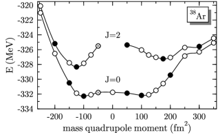
Figure 1: Energy landscapes for $J=0$ and $J=2$ angular-momentum projected states in ³⁸Ar. The open circles show the $q$ values of the calculated configurations, with lines drawn to guide the eye. Solid circles are ones included in the mixed configuration calculations for the global survey.

II.3 Matrix elements of the quadrupole operator

The calculation of the quadrupole moments of projected states requires the calculation of all components of the quadrupole tensor. $Q_{2\pm 1}$ and $Q_{2\pm 2}$ are of course exactly zero for axial mean-field states with the $z$ axis as symmetry axis as chosen here, but they have non-vanishing transition matrix elements between a rotated and an unrotated state.

The detailed expressions for the quadrupole operator and its projected matrix elements can be found in appendix A. For axial states, as used here, only the matrix elements of $\hat{Q}_{20}$ and the real part of the matrix elements of $\hat{Q}_{21}$ and $\hat{Q}_{22}$ need to be calculated, which simplifies the computational task.

To calculate matrix elements of the quadrupole operator $\hat{Q}_{2\mu}$, some modifications of the GOA parameterization are necessary since the functional behavior of the operator depends on its azimuthal angular momentum $\mu$. In particular, for the matrix element of $Q_{2\pm 1}$, the form $F(\beta)=\sin^{2}(\beta)$ used in the polynomial expansion of Eq. (II.2.1) is not topologically correct. We therefore define a topGOA by taking $d^{2}_{\mu 0}(\beta)$ for the argument of the polynomial expansion

$$\Re\big{\{}\langle q|\hat{R}_{\beta}\hat{Q}_{2\mu}|q^{\prime}\rangle\big{\}}$$ (9)

$$= \langle q|\hat{R}_{\beta}|q^{\prime}\rangle_{t}\left[a_{0}+a_{2}d^{2}_{\mu 0}(\beta)+a_{4}\left(d^{2}_{\mu 0}(\beta)\right)^{2}\right],$$

where the coefficients of the polynomial $a_{i}$ depend on $q,q^{\prime}$. As with the other matrix elements, it is important to include the point at $\beta=\pi/2$ when $q$ and $q^{\prime}$ have opposite signs.

There is an additional complication compared to the norm and Hamiltonian kernels. While for these scalar operators the kernels (7) and (II.2.1) are invariant under exchange of $|q\rangle$ and $|q^{\prime}\rangle$, this is not the case for the quadrupole operator, where $\langle q|\hat{R}_{\beta}\hat{Q}_{2\mu}|q^{\prime}\rangle$ is not equal to $\langle q^{\prime}|\hat{R}_{\beta}\hat{Q}_{2\mu}|q\rangle$. To avoid the explicit calculation of both, we express the latter matrix elements as a weighted sum of the former using angular-momentum algebra and the symmetry properties of the SCMF states promesse . A separate topGOA is then set up to calculate the projected matrix element from the $\langle q^{\prime}|\hat{R}_{\beta}\hat{Q}_{2\mu}|q\rangle$. It has to be noted, however, that the difference plays a role only for transition matrix elements between states with different angular momentum. As we are interested here in $2^{+}\to 0^{+}$ transitions only, the topGOA for matrix elements with exchanged arguments is needed for $\mu=0$ only, Eq. (15).

An example for the fits of the integrand is shown in Fig. 2 for ⁵²Cr at a deformation of $q=q^{\prime}=150$ fm². Starting from the bottom panel, the three panels show the rotated overlap matrix element $\langle q|\hat{R}_{\beta}\hat{Q}_{2\mu}|q\rangle$ for $\mu=0$, 1 and 2 respectively. The open circles are the points used to evaluate the integral by a 12-point Gaussian quadrature, as it would be used in a calculation for the complete low-energy spectroscopy of this nucleus. The solid circles are the points used for the topGOA fit, the resulting curves being indicated by lines. The agreement is excellent; the error associated with the topGOA is typically less than 1 $\%$ for the $\mu=0$ matrix element. This is the only one needed to calculate the $B(E2)$ value of the $2^{+}\to 0^{+}$ transition (see appendix A). The middle panel shows the integrand for the $Q_{21}$ operator. In effect, only the middle point can be used for the fit because the integrand vanishes at $\beta=0$ and $\pi$. Nevertheless, this approximation works rather well. It is less accurate for some non-diagonal matrix elements, particularly for matrix elements connecting configurations with very different deformations which are needed to describe soft nuclei. The top panel shows the matrix element for the operator $Q_{22}$. Here there are effectively two points to determine the topGOA fit.

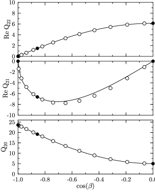
Figure 2: The matrix element $\langle q|\hat{R}_{\beta}\hat{Q}_{2\mu}|q\rangle$ for the nucleus ⁵²Cr at an intrinsic deformation of $q=150$ fm². The open circles show the points used for evaluating the integral by a 12-point Gaussian quadrature. The solid circles show the points used for the topGOA, and the resulting fit. The three panels show the results for $\mu=0,1$ and 2 going up from the bottom panel.

To test this approximation further, we have compared the topGOA quadrupole matrix elements with the matrix elements obtained by a full integration for a variety of nuclei and deformations. The result is shown in Fig. 3. One can conclude that Eq. (9) is of sufficient accuracy for our purpose.

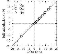
Figure 3: Comparison of the topGOA and full calculation for $Q_{2\mu}$ for various nuclei and deformations.

II.4 Configuration mixing

As mentioned above, we typically compute about $N_{q}=20$ SCMF configurations to construct the energy landscape. For many nuclei, however, only about half that number can be kept in the configuration mixing calculation due to ill-conditioned norm matrices when the space is overcomplete. Nevertheless, the full configuration mixing calculation requires to compute about 50 projected matrix elements, which is beyond our computational resources for a study of several hundred nuclei. In Ref. Ben04a , a GOA was developed for a coordinate corresponding to the deformation $q$, permitting calculations to be made to the needed accuracy only using the diagonal and subdiagonal elements of the configuration mixing matrix, i.e. about $2N_{q}$ projected matrix elements. Unfortunately, the demands on the approximation are more severe when calculating quadrupole matrix elements between states of different angular momentum. The matrix element can change sign, depending on the deformations. For matrix elements connecting different manifolds of states ($0^{+}$ and $2^{+}$), there is no diagonal element to anchor the GOA.

Lacking a reliable GOA to determine the off-diagonal quadrupole matrix elements, we took another approach to simplify the configuration mixing calculation. The number of configurations has been reduced for each nucleus to a number small enough to make a global calculation feasible but large enough to have a sufficient accuracy on the energy of the lowest $0^{+}$ and $2^{+}$ states. Since we have to deal with energy curves of very different topologies, some care must be taken into the selection of points. The procedure that we have followed is explained in appendix B. The number of selected configurations varies from 3 to 10, but is most often equal to 6. We have therefore labeled this approximation HW-6.

The points selected for ³⁸Ar are shown in Fig. 1 as black circles. In this case, the single-configuration MAP energy of the ground state is $E_{0}(\text{MAP})=-332.25$ MeV, as quoted in the last section. The gain in energy from configuration mixing with the large set of configurations (11 in this case) is $E_{0}(HW)-E_{0}(\text{MAP})=-332.69+332.25=-0.44$ MeV. This is to be compared with $-332.61+332.25=-0.36$ MeV for the HW6 space. The error, $0.08$ MeV, is within our targeted limit of accuracy. For the $J=2$ projected wave functions, the energy gain by the HW treatment is $-0.68$ MeV and the error of the 6-configuration truncation is 0.07 MeV with the same sign as in the ground state energy. With our present computer resources, we were able to test the HW6 truncation for about 100 nuclei. The $2^{+}$ excitation energies computed both ways are compared in Fig. 4. The approximation reproduces the energies to an r.m.s. accuracy of better than 0.1 MeV. The worst cases are two nuclei with coexisting minima at low excitation energy that are separated by very low barriers, ¹⁸⁸Pb and ¹⁹⁰Pb, visible as points off the line at the bottom left-hand corner of the graph.

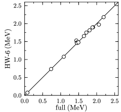
Figure 4: Comparison of $2^{+}$ excitation energies for the full and the HW-6 bases.

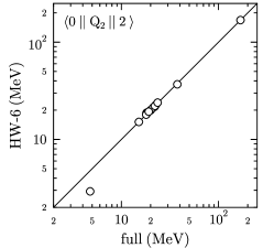
Figure 5: Comparison of the reduced matrix element $\langle 0||\hat{Q}_{2}||2\rangle$ for the $2^{+}\to 0^{+}$ transition obtained within the full and the HW-6 bases.

The same comparison for the reduced matrix element of the $2^{+}\to 0^{+}$ transition is shown in Fig. 5. The agreement is very good except for the light Pb isotopes, ¹⁸²Pb, ¹⁸⁸Pb, and ¹⁹⁰Pb. Among the nuclides, the light Pb isotopes are rather singular and we shall examine ¹⁸⁸Pb in more detail in the next section. Overall, the accuracy of the HW-6 approximation is more than adequate for the present global survey.

III Some examples

In this section we shall examine the results for a sample of nuclei with energy maps of different topologies: a light doubly-magic system, ⁴⁰Ca; a heavy doubly-magic system, ²⁰⁸Pb; a transitional nucleus near magicity, ³⁸Ar; a soft nucleus exhibiting triple shape coexistence, ¹⁸⁸Pb; and a well-deformed heavy nucleus, ²⁴⁰Pu. We first examine the results of the MAP approximation.

III.1 MAP

The MAP approximation is a variation after projection method within the very limited subspace defined by the axial quadrupole operator. For each $J$-value, one finds the configuration leading to the lowest energy, which thus could be different for $J=0$ and $J=2$. The results for the observables of interest are presented on the first line of Table 1, together with the experimental data on the last line ra02 . In all cases, except ¹⁸⁸Pb, the calculated 2⁺ excitation energy is too high. For ³⁸Ar, this overestimation has been attributed to the structure of the state Ben03a . It is indeed very likely predominantly a broken-pair two-quasiparticle configuration, where the two occupied magnetic substates in the proton $d_{3/2}$ shell below the $Z=20$ gap are coupled to $J=2$. A rough estimate for its excitation energy is provided by two times the proton pairing gap, which leads to an excitation energy close to the experimental one. The description of this state requires the breaking of time-reversal reversal invariance and of axial symmetry in the SCMF, which is outside of what we can currently handle within our beyond-mean-field approaches. The excited state in the ⁴⁰Ca is of a different nature. Since, within the shell model, one does not obtain low-lying even-parity excitations, this state has been famous in the literature as an early example of shape coexistence. The first excited state of ⁴⁰Ca is a $0^{+}$ which is the head of an intruder deformed band. A detailed study of this nucleus with the full projected GCM has indeed obtained such a band Ben03a . Although the SLy6 interaction was used in that case, the results that we find here are very similar.

The next nucleus ¹⁸⁸Pb shows still another kind of behavior. It is a nucleus with several coexisting minima, which are separated by tiny barriers only. This isotope has been studied in detail in Ref. Ben04b with several other neutron-deficient Pb isotopes. Under the MAP approximation, the ground state is obtained from a configuration close to sphericity, while the minimum for the first $2^{+}$ is strongly oblate. The next example, ²⁰⁸Pb, is a heavy doubly magic nucleus. Simple shell model considerations give already an idea of what should be the dominant component of the first 2⁺  excitation. It can be obtained by promoting a neutron from the occupied $i_{13/2}$ shell to the unoccupied $g_{9/2}$ shell, or a proton from the $h_{11/2}$ shell to the $h_{9/2}$ shell. The single-particle energy differences in the spherical mean-field configuration are 6.4 and 5.9 MeV, respectively. The MAP energy is 2 MeV higher than the particle-hole energy. Again, like in the case of ³⁸Ar, the relevant configurations are broken-pair two-quasiparticle states outside our configuration space. The last nucleus in the table, ²⁴⁰Pu, is highly deformed. Its character is already seen in the SCMF wave function, which has an intrinsic mass quadrupole moment of $q=3000$ fm², of which 1145 fm² is taken up by the electric quadrupole moment. Assuming that the wave function corresponds to a rigid rotor, Eq. (21), one obtains a transition quadrupole moment $\langle 0||\hat{Q}_{2}||2\rangle=361$ $e$ fm² in agreement with experiment. The MAP approximation does not change matters; the minimizing $q$ of the $J=0$ and $J=2$ projected states are very close to that of the SCMF ground state. However, one sees from the table that the excitation energy of the 2⁺ state is too high by nearly a factor of two. This is another well-known problem, which has been seen in virtually all calculations using methods similar to ours: much better agreement would be obtained using the cranked HFB method to generate a wave function for the $2^{+}$ state.

Table 1: Results for some selected nuclei. The reduced transition matrix element and the spectroscopic quadrupole moment are defined in Eqs. A and (18), respectively; the relation to the $B(E2)$ is given in Eq. (16). The theoretical values for ¹⁸⁸Pb from Ref. Ben04b assume that the ground state is spherical and the excited state is oblate.

nucleus	source	$E_{ex}$	$\langle 0||\hat{Q}_{2}||2\rangle$	$Q_{c}$
		(MeV)	($e$ fm2)	($e$ fm2)
38Ar	MAP	3.9	20.4	-22.8
	HW-full	3.7	19.9	3
	HW-6	3.8	19.1	-10
	Ref. Ben03a	3.6	22.8	6.9
	exp.	2.17	11.4
40Ca	MAP	5.4	23.8	34.6
	HW-full	5.0	18.2	-6
	HW-6	5.3	16.7	1
	Ref. Ben03a	5.4	23.7	2.2
	experiment	3.90	9.9
188Pb	MAP	0.17	192	173
	HW-full	0.54	102	170
	HW-6	0.22	188	180
	Ref. Ben04b	0.93	71	110
	experiment	0.72
208Pb	MAP	7.9	99	70
	HW-full	7.0	84	1
	HW-6	7.1	81	6
	experimental	4.09	55
240Pu	MAP	0.076	377	-341
	HW-full	0.076	377	-341
	HW-6	0.076	377	-341
	Ref. Ben04c	0.083	377	-340
	experimental	0.043	361

III.2 HW and HW-6

We now examine the effects of configuration mixing on the properties of the 2⁺ state, which are also given in Table 1. Mixing in the large (“full”) configuration space significantly reduces the energy in two cases, ⁴⁰Ca and ²⁰⁸Pb, raises the energy in one case, ¹⁸⁸Pb, and has little or no effect in two cases, ³⁸Ar and ²⁴⁰Pu. The insensitivity for ²⁴⁰Pu is to be expected since strongly deformed rotors do not have large shape fluctuations, see the detailed discussion for this example in Ref. Ben04c . Including shape fluctuations improves the description of a soft nucleus as ¹⁸⁸Pb. We see that the full calculation (HW) produces an excitation energy that approaches the experimental value. In all the cases where the fluctuations change the energy, the change goes in the right direction and decreases the theoretical error.

On the third line of Table 1, we show the effect of the truncation of the configuration space in the HW-6 approximation. In all but the case of ¹⁸⁸Pb the energies are close to the full HW results. The light Pb isotopes are quite exceptional, but we saw in the previous section that HW-6 is reliable enough for a global survey. The next line in Table 1 shows results from other calculations. The reported calculations of ³⁸Ar, ⁴⁰Ca,¹⁸⁸Pb and ²⁴⁰Pu were done with the full projected GCM without approximations, using the same computer codes as here, but with a slightly different energy functional. We see that the results are qualitatively similar to what we found, indicating a mild sensitivity to the specific energy functional.

We now discuss the quadrupole matrix elements in more detail. The simplest case is ²⁴⁰Pu, which, as discussed above, behaves very much like a rigid rotor. In the rotor limit, the transition quadrupole matrix element is proportional to the spectroscopic quadrupole moment of the 2⁺ state. The relation is given in appendix A, $Q_{c}/\langle 0||\hat{Q}_{2}||2\rangle\approx 0.9$. We see from the table that this is well satisfied for all calculations of ²⁴⁰Pu. For the non-deformed nuclei, the spectroscopic quadrupole moment is small, as would be expected for a spherical vibrator. In the four cases given in Table 1, the HW and HW-6 transition matrix elements, although overestimating the experimental data, are better than a factor two, even in cases where the dominant component of the $2^{+}$ appears to be incorrect. This is probably related to the fact that the quadrupole moment is a bulk property that is entirely determined by the overall distribution of the local density, while the energy is sensitive to the detailed structure and occupation of each single-particle wave function. Note also that allowing spreading of the wave functions over several configurations improves the MAP result.

IV Global performance

We carried out the MAP and HW-6 calculations on even-even nuclei with known binding energies, excluding light nuclei with $N$ or $Z<8$. This is the set studied in Ref. Ben06 . Of these, 522 have known 2⁺ excitation energies. These energies range from 39 keV to 6.9 MeV, thus spanning more than 2 orders of magnitude. The theoretical numbers span the same range, but as we saw in the last section there can easily be a factor two error in specific cases.

In view of the results of the previous section, we have excluded from the full set of nuclei the ones for which one can have suspicion about our approximation scheme. To identify these nuclei, we have compared our present HW-6 results with the global calculation performed earlier where the number of configurations included in the calculation of the ground state was not limited. We eliminate all the nuclei for which the difference between both calculations for the energy of the $0^{+}$ ground state was larger than 250 keV. The selected set of nuclei does not include ¹⁸⁸Pb, and similar nuclei which are too soft to be represented by either a MAP calculation or a small number of quadrupole configurations. Out of the $522$ nuclei calculated, there remain after selection 359 .

IV.1 Global results

Because the energies span a broad range and the error can be large, we will quote the aggregated results for the logarithm of the ratio of the theoretical to experimental energies,

$$R_{E}=\log(E_{th}/E_{exp}).$$ (10)

A histogram of this quantity for the entire set of nuclei is shown in Fig. 6, displaying the MAP results in the lefthand panel and the HW-6 results in the righthand panel. We see that the results of both methods tend to be too high, with a fairly broad distribution containing both negative and positive errors. Quantitative statistical measures of the distribution are given in Table 2.

Table 2: Statistics for the performance of the MAP and HW-6 calculations.

Selection	Number	observable	theory	average	dispersion
of nuclei	of nuclei			$\langle R\rangle$	$\langle(R-\langle R\rangle)^{2}\rangle^{1/2}$
all	359	$E_{20}$	MAP	0.28	0.49
	359	”	HW-6	0.51	0.38
	212	$\langle 0||Q_{2}||2\rangle$	MAP	0.12	0.22
	212	”	HW-6	0.09	0.23
deformed	135	$E_{20}$	MAP	0.20	0.36
	135	”	HW-6	0.27	0.33
	93	$\langle 0||Q_{2}||2\rangle$	MAP	0.10	0.10
	93	”	HW-6	0.10	0.11
semi magic	58	$E_{20}$	MAP	0.53	0.55
	58	”	HW-6	0.58	0.31
	28	$\langle 0||Q_{2}||2\rangle$	MAP	0.37	0.24
	28	”	HW-6	0.35	0.23

The average MAP error is found to be $\langle R_{E}\rangle\approx 0.28$ but the average of the absolute value of the error is much larger, $\langle|R_{E}|\rangle=0.48$, corresponding to an error of the order of 66 $\%$. The dispersion around the average is also quite large: $\langle(R_{E}-\langle R\rangle)^{2}\rangle^{1/2}=0.49$. With such a dispersion, an error larger than a factor of two is not unusual. Specifically, of the 359 nuclei in the data set, 19 $\%$ have a calculated energy too large by a factor of two and 4 $\%$ are too low by the same factor. Fig. 7 shows a scatter plot of the MAP and the experimental energies. One sees that the energies are overestimated for most nuclei, and in particular for nuclei with either a low or a high excitation energy of the $2^{+}$, where the nuclei are predominantly deformed or magic, respectively. This is consistent with what we saw in the examples of the previous section. For excitation energies in the range 200 keV to 1 MeV, there is no obvious trend in error of the MAP calculation.

Figure 6: Histogram of the logarithmic errors $R_{E}$ of the energies of the first excited 2+ states (solid) and the logarithmic errors $R_{Q}$ of the reduced matrix elements $\langle 0||\hat{Q}_{2}||2\rangle$ (dashed) for the 359 even-even nuclei included in our survey (solid). The two panels show the results of the MAP theory (left) and the projected GCM in the HW-6 approximation (right).

Figure 7: Scatter plot comparing the theoretical and experimental 2⁺ excitation energies of the 359 nuclei included in the survey. The two panels show the results for the MAP method on the left and the HW-6 approximation on the right.

As can be seen in Table 2, the mean error of the HW-6 calculation is significantly larger than the MAP error, with an average around $\langle R_{E}\rangle\approx 0.51$. The dispersion around the average is however lower and the average of the absolute value of the error is only slightly larger than for the MAP results (0.54 compared to 0.48). In Fig. 7 are plotted the HW-6 excitation energies as a function of the experimental data. One can see that in most cases, the 2⁺ excitation is overestimated and this tendency is much more pronounced than for the MAP results. In fact, in many cases, the HW-6 $2^{+}$ energy is larger than the MAP one. This increase when the configuration mixing correlations are included means that the correlation energies predicted by our method are larger in the ground state than in the $2^{+}$ state. There can be many origins to this difference in correlation energies. The lack of triaxial configurations certainly affects more deeply the states with $J\neq 0$ since for these states the spherical point does not contribute and the coupling between prolate and oblate configurations is disfavored. It is also clear that the MAP procedure is better defined numerically than the HW-6 one. In each case, we are sure to have determined for both $J=0$ and $J=2$ the quadrupole moment giving the minimal energy after projection. For the configuration mixing, the fact that we have excluded the nuclei for which the $J=0$ energy is too different from our previous global calculation makes the determination of the $0^{+}$ energy reliable. We do not have a similar check for $J=2$ and there are cases where the number and the spacing of points taken for $J=2$ is not fully adequate and the energy of this state less accurate.

While the energies are not accurately predicted, the quadrupole properties come out much better and with rather similar errors for both the MAP and HW-6 results. It is well known that the intrinsic quadrupole moments of deformed nuclei are rather insensitive to the details of the energy functional, and indeed we found that the quadrupole transition matrix element is much better determined overall than the energy. The dashed histograms in Fig. 6 show the logarithmic ratio $R_{Q}$ of the reduced quadrupole transition matrix elements $\langle 0||\hat{Q}_{2}||2\rangle$ (see appendix A). The average error is only 0.12 for the MAP calculation, corresponding to matrix elements that are 15% too large and 0.09 for the HW-6 results (error of 9%). The r.m.s. spread is also reduced. For example, in the MAP case, it takes the value 0.22 corresponding to transition matrix elements that are -10% to +46% of the data. We will now analyze separately the different kinds of nuclei. To that aim, we divide the nuclei by type and examine in more detail the performance for subgroups that are deformed, doubly-magic, and singly-magic.

IV.1.1 Deformed nuclei

We first have to define a criterion to select which nuclei should be considered deformed. Obviously, there is no rigorous division of nuclear types, and any division is somewhat arbitrary. One possibility is to make a selection on the basis of the intrinsic quadrupole moment of the MAP ground state, taking into account overall size effects by using the geometric shape parameter $\beta_{2}$ [defined in Eq. (23)] to make the selection. This criterion will catch many light nuclei along with the usual nuclei in the lanthanide and actinide regions. One should add the criterion of rigidity to the selection as well to eliminate the nuclei that have large fluctuations in shape. In this sense, what we are seeking to categorize are nuclei that behave like rigid rotors. A criterion that makes a nice selection is to demand that the average deformation $\bar{\beta}_{2}$ is large than the r.m.s. fluctuation about the average, $\bar{\beta}_{2}>\langle(\beta_{2}-\bar{\beta}_{2}\rangle^{1/2}$. These quantities are computed using the full HW wave functions of Ref. Ben06 , and the criterion selects 134 deformed nuclei from our set of 359. Their energies are plotted as a function of neutron number in Figs. 8 with the MAP results in the lefthand panel and the HW-6 results in the righthand panel. The two plots are rather similar.

Figure 8: 2⁺ excitation energies in deformed nuclei as a function of neutron number: MAP in left panel; HW-6 approximation in right panel. Experimental data are shown as diamonds.

We see that the predictions are too high for the actinides, while on the average they are quite reasonable for rare earth nuclei. The statistic on the errors for deformed nuclei is summarized in Table 2. One can see that the average error is smaller than for the full set. The dispersion in the error is the same for both the MAP and the HW6 approximations, so, the axial quadrupole correlations do not seem to be the source of the nucleus-to-nucleus fluctuations of error.

Fig. 9 shows the ratio of theoretical to experimental quadrupole transition matrix elements for the deformed nuclei. Here the actinide nuclei come out very well. There is more fluctuation in the rare earth and the light nuclei that qualify as strongly deformed but the overall results are quite satisfactory.

Figure 9: Ratio of theoretical and experimental transition quadrupole matrix elements $\langle 0||\hat{Q_{2}}||2\rangle$ in deformed nuclei, as a function of neutron number.

Figure 10: 2⁺  excitation energies near magic nuclei, as a function of neutron and proton numbers. MAP and HW6 results are shown by points connected with lines, while experimental data are shown by filled diamonds.

Figure 11: Ratio of theoretical and experimental quadrupole transition matrix elements near magic nuclei as a function of neutron and proton numbers. MAP and HW6 results are shown as points connected by dotted and solid lines, respectively.

IV.1.2 Magic and semi-magic nuclei

We now turn to doubly- and singly-magic nuclei, which present quite different problems for the theory. The comparison between theoretical and experimental 2⁺ excitation energies of six doubly magic nuclei is shown in Table 3. The MAP and HW-6 energies are too high in three cases and too low for the other three, preventing us from drawing any general conclusions.

Table 3: Excitation energy of the first $2^{+}$ state in MeV for doubly magic nuclei.

$N$	$Z$	exp.	MAP	GCM
20	20	3.9	5.4	5.4
28	20	3.8	2.7	2.7
28	28	2.7	2.0	2.2
82	50	4.0	6.3	5.8
126	82	4.1	7.9	6.7

There are 71 semi-magic nuclei in our compilation, requiring that either the neutron or the proton number equal to 28, 50, 82 or 126. Graphs of 2⁺ excitation energies are shown in Figs. 10 as a function of neutron number and proton number. MAP results are shown by the points connected with solid lines, HW-6 results with long dashed lines, and experiment by shorter dashed lines. For both MAP and HW-6, the excitation energy has a peak at the doubly-magic nuclides which decreases gradually going away from that nucleus. In contrast, the experimental peak is a sharp spike at the doubly-magic nuclides. This deficiency of the theory is related to the absence of broken-pair two-quasiparticle excitations that can give a lower non-collective $2^{+}$ state as we saw already in the example of ³⁸Ar. As to be expected from this discussion, the statistical measures are much poorer for this class of nuclei. The average calculated energy is 50% higher than experiment and the average calculated transition quadrupole moment is 2.2 times the experimental value.

Fig. 11 compares the theoretical and experimental transition quadrupole moments in semimagic and magic nuclei. The data is much more meager than for the energies, but one can see that the theory nearly always is too high. As discussed earlier, this is to be expected when the lowest 2⁺ is not collective.

IV.2 Discussion

In view of their restricted form and of the way they have been fitted to selected experimental data, the current energy functionals are certainly too limited and, as discussed in Ben06 ; Ben06b , present deficiencies which are at the origin of some of the discrepancies between our calculations and experiment. However, the present analysis clearly points also to deficiencies of the variational space that is used, that affect more excitation energies than quadrupole moments.

One can expect that our configuration space spanned by axial quadrupole SCMF wave functions covers the correlations that dominate the description of the $0^{+}$ ground states of even-even nuclei. On the contrary, there are several competing possibilities to construct a low-lying $2^{+}$ state, some of them being completely absent from our description:

1. a broken-pair two-quasiparticle excitation within a partly-filled $j$ shell with an excitation energy of about two times the pairing gap (for example near-magic nuclei like ³⁸Ar)

2. a broken pair two-quasiparticle excitation involving two different $j$ shells, one occupied, the other unoccupied, with an excitation energy of about the gap between the $j$ shells involved (for example doubly-magic nuclei as ²⁰⁸Pb)

3. a collective vibrational state

4. a collective rotational state (for example for well-deformed rare-earth and actinide nuclei)

The states corresponding to such pure configurations should of course be mixed in actual nuclei. The projected GCM of axially deformed SCMF states that correspond to HFB vacuua, as it is used here, cover only the latter two of these configurations. In nuclei where the lowest $2^{+}$ state is dominated by broken-pair two-quasiparticle states, the $2^{+}$ state that our method enables us to describe corresponds to a higher-lying collective $2^{+}$ state. On the other hand, the number of nuclei for which the lowest $2^{+}$ state is indeed dominated by a broken-pair two-quasiparticle state can be expected to be small, and restricted to the immediate vicinity of doubly-magic nuclei. In nuclei where the first $2^{+}$ is expected to be collective, either vibrational, or rotational,the excitation energies are also on the average too high. This result confirms on a large scale previous studies performed with similar methods for smaller sets of nuclei Ben03a ; Ben04b ; Ben04c ; Ben05b ; ro02 ; Rod02a ; Egi04a

An obviously missing degree of freedom is triaxiality, as our configuration mixing contains only two out of the five degrees of freedom of the quadrupole tensor. On the one hand, it is well-known that many transitional nuclei are $\gamma$ soft. A recent global study based on a semi-microscopic method has even indicated that the potential energy surface of many transitional nuclei might have a triaxial minimum Moe06a , although with an energy gain that remains very small. It has also been shown Har82a that in some cases triaxial quadrupole configurations can be more favorable after angular-momentum projection than axial configurations. The effect of triaxiality on excitation energies has also been studied with the help of an effective five-dimensional Bohr Hamiltonian derived from mean-field calculations using the Gogny force Gir78a ; li99 or a Skyrme interaction Pro04a . A similar overestimation of the lowest $2^{+}$ energy as in the present study has been found. Therefore, if the effects of triaxiality are certainly non-negligible on total energies, it is unclear whether they will improve excitation energies.

Table 4: Excitation energy of the first $2^{+}$ state in MeV for Zn isotopes.

$N$	Expt.	MAP	HW-6	cranked SCMF
30	0.89	1.85	1.89	1.35
32	0.56	2.36	1.94	0.90
34	0.61	1.56	1.81	0.41
36	0.60	1.09	1.71	0.37
38	0.73	1.88	1.95	0.41
40	1.50	2.64	2.33	0.80

The effect of triaxial quadrupole deformations on excitation energies is not obvious. The method that we use has however clearly an artifact which favors the $0^{+}$ energy with respect to the $2^{+}$: the mean-field is optimized to describe the ground state and not excited states. An obvious improvement would be to perform an exact variation after projection (VAP), performed separately for $J=0$ and $J=2$. Variation after projection on angular momentum starting from effective interactions and with a full model space does not seem however within computational possibilities in a near future. A more modest approach would be to use the self-consistent cranking method to optimize separately the intrinsic configurations describing different spin states. This can be done by introducing in the mean-field equations a constraint on the projection of the angular momentum. It has been shown that the self-consistent cranking method is an approximation of a variation after projection on angular momentum for well deformed nuclei RS80 . Such an approach will necessarily improve the description of the $2^{+}$ states and decrease their excitation energy.

Even for nuclei which are not deformed, the effect of a cranking constraint, which breaks time-reversal invariance can only go in the right direction, although it is not clear a priori that the introduction of two-quasiparticle excitations would not be even more important. To give some insights into the effect of a cranking constraint for isotopes which are not deformed, we show in Table 4 the results of MAP, HW-6 and cranked SCMF calculations together with the experimental data for some neutron-rich Zn isotopes. The cranked SCMF calculations were done with the method described in Ref. 95e and with the same effective interaction as for the other calculations of this study. Both MAP and HW-6 results strongly overestimate the experimental energies, the MAP being even rather irregular in its predictions. The cranking results are given in the last column. The $2^{+}$ excitation energy in this case is the difference between the mean-field ground state energy and that of the state obtained with a cranking constraint $J_{z}=2$. One sees that the energies are significantly lower compared to the calculations where time reversal invariance is imposed. The numbers that are obtained can even be lower than the experimental data. One cannot go too far in the interpretation of these results which do not include any projections. However, they show that an optimization of the $2^{+}$ wave function with a cranking constraint might have a significant effect going in the right direction for all nuclei.

Figure 12: Chart of nuclides showing the even-even nuclei for which the excitation energy of the first 2⁺ state is known. Nuclei for which the MAP calculation is in error by more than a factor of two are shown by solid triangles. Upper panel: theory too low; lower panel: theory too high.

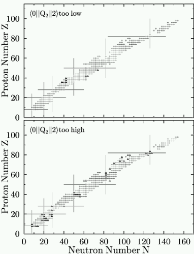
Figure 13: Chart of nuclides showing the even-even nuclei for which the transition quadrupole moment to the first 2⁺ state is known. Nuclei for which the MAP calculation is in error by more than a factor of two are shown by solid triangles. Upper panel: theory too low; lower panel: theory too high.

It remains to verify what will happen when exact projection and configuration mixing will be performed, but the perspective of a global qualitative improvement of the present results seems reasonable. The generalization of the method used here for use with cranked SCMF states requires a similar, even greater, effort as the generalization to triaxial shapes: the cranking constraint induces non-axial intrinsic currents, even when the overall density distribution remains axial. The broken-pair two-quasiparticle states discussed above require a similar generalization of the spatial symmetries in the projected GCM as the cranked HFB vacuum.

V Summary and outlook

This is the first systematic survey of the $2^{+}$ excitations of even-even nuclei in the framework of a mean-field based method including symmetry restoration and starting from an effective energy functional. The effort necessary for this task is significantly larger than the one required for our earlier study on the ground states of these nuclei Ben06 , both for the representation of the collective $2^{+}$ states, and to obtain a sufficient precision for the matrix elements of the quadrupole operator. For several nuclei we could not reach an acceptable precision, so that the subsequent analysis was performed on a reduced set of data.

Qualitatively the excitation energies and $B(E2)$ values track the data for the great majority of the 359 nuclei studied. However, predicted energies and $B(E2)$ values are systematically too high, and there are a number of cases where key ingredients are clearly missing. The worst cases, where the observable is more than a factor of two in error, are marked on the charts of nuclides in Figs. 12 and 13. One can discern some patterns that point to deficiencies in the energy functional and in the GCM methodology that both may be correctable.

Many of the outlying points in Fig. 12 are cases where the theory predicts a nearly spherical nucleus while the data show it to be deformed, or vice versa. An example is ⁸⁰Zr, predicted spherical but obviously deformed in view of the very low excitation energy of its first $2^{+}$. The shell effect predicted by our effective interaction for ⁸⁰Zr is clearly too large, as already analyzed in our study of ground-state correlations Ben06 . All conclusions of Ref. Ben06 about necessary future work on the effective interactions and the model space also apply here, see also Ben06b .

Our calculation reproduces rather nicely the quadrupole transition matrix elements between the first $2^{+}$ and the ground state: the average error that we obtain is around 25$\%$. The situation is less satisfactory for the excitation energies of the first $2^{+}$ states, which is nearly always overestimated. This seems to be a general problem that has been noticed before in many calculations using Skyrme and Gogny interactions. As argued above, we relate this deficiency mainly to the current restrictions of the variational space that we use. To overcome this limitation, the extension of the variational space to include triaxial states, and cranked SCMF states is highly desirable. Work in that direction is underway. The enormous increase in computational time, however, will not permit its large-scale application right away.

Appendix A Matrix elements of the quadrupole operator

For reference, we quote the definitions of the quadrupole matrix elements and simplified versions of the formulas from Ref. Ben03a for calculating them. For the sake of simple notation, we will give all expressions, where applicable, for matrix elements between two different SCMF configurations, $|q\rangle$ and $|q^{\prime}\rangle$. The generalization to GCM states with their weighted summation is straightforward as it does not affect the angular momentum algebra.

The electric quadrupole operator is defined as

$$\hat{Q}_{2\mu}=e\sum_{p}r^{2}_{i}Y_{2\mu}(\hat{r}_{i})$$ (11)

We start with Eq. (A7) of Ref. Ben03a for the reduced matrix element of the quadrupole operator between two projected axial states

$$\langle Jq||\hat{Q}_{2}||J^{\prime}q^{\prime}\rangle = \frac{\sqrt{2J+1}(2J^{\prime}+1)}{\mathcal{N}_{Jq}\mathcal{N}_{J^{\prime}q^{\prime}}}\sum_{\mu=-2}^{+2}\langle J^{\prime}02\mu|J\mu\rangle$$

$$\times\int_{0}^{1}\!d\cos(\beta)\,d^{J}_{0\mu}(\beta)\;\langle q|\hat{R}_{\beta}\hat{Q}_{2\mu}|q^{\prime}\rangle$$

where $J$ and $J^{\prime}$ are assumed to be integer and even. $\hat{R}_{\beta}$ is the rotation operator, $d^{J}_{\mu\kappa}(\beta)$ is the Wigner $d$-function, and $\mathcal{N}_{Jq}$ is the normalization of the $J$-projected SCMF state, Eq. (6). The reduced matrix element on the left-hand side is defined as Var88a

$$\langle JMq|\hat{Q}_{2\mu}|J^{\prime}M^{\prime}q^{\prime}\rangle=\frac{\langle J^{\prime}M^{\prime}2\mu|JM\rangle}{\sqrt{2J+1}}\langle Jq||\hat{Q}_{2}||J^{\prime}q^{\prime}\rangle.$$ (13)

Equation (A) can be even simplified further using the symmetries of the Wigner functions and the quadrupole operators

$$\langle Jq||\hat{Q}_{2}||J^{\prime}q^{\prime}\rangle = \frac{\sqrt{2J+1}(2J^{\prime}+1)}{\mathcal{N}_{Jq}\mathcal{N}_{J^{\prime}q^{\prime}}}\bigg{(}\langle J^{\prime}020|J0\rangle\int_{0}^{1}\!d\cos(\beta)\;d^{J}_{00}(\beta)\;\langle q|\hat{R}_{\beta}\hat{Q}_{20}|q^{\prime}\rangle$$ (14)

$$\qquad\qquad\qquad+2\sum_{\mu=1}^{2}\langle J^{\prime}02\mu|J\mu\rangle\int_{0}^{1}\!d\cos(\beta)\;d^{J}_{0\mu}(\beta)\;\Re\{\langle q|\hat{R}_{\beta}\hat{Q}_{2\mu}|q^{\prime}\rangle\}\bigg{)},$$

which serves as the starting point for the GOA set-up in section II.3.

To compute the matrix element for the $2^{+}\to 0^{+}$ transition, one evaluates the above formula with $J=0$ and $J^{\prime}=2$. Only $\mu=0$ contributes in this case and the result is

$$\langle 0q||\hat{Q}_{2}||2q^{\prime}\rangle=\frac{\sqrt{5}}{\mathcal{N}_{2q}\mathcal{N}_{0q^{\prime}}}\int^{1}_{0}\!d\cos(\beta)\;\langle q|\hat{R}_{\beta}\hat{Q}_{20}|q^{\prime}\rangle.$$ (15)

The $B(E2)$ for the transition is related to the reduced matrix element by Var88a

$$B(E2,2^{+}\to 0^{+})=\frac{1}{5}\;\langle 0q||\hat{Q}_{2}||2q^{\prime}\rangle^{2}.$$ (16)

The other matrix element of interest is the spectroscopic quadrupole moment of the $J=2$ excited state, defined as

$$Q_{c}=\sqrt{\frac{16\pi}{5}}\langle 22q|\hat{Q}_{20}|22q^{\prime}\rangle.$$ (17)

In this case the sum over $\mu$ cannot be avoided. The final result is

$$Q_{c}=-\frac{5}{\mathcal{N}_{2}^{2}}\left(-\frac{2}{7}M_{0}+\frac{2}{7}M_{1}+\frac{4}{7}M_{2}\right)$$ (18)

where

$$M_{\mu}=\sqrt{\frac{16\pi}{5}}\int^{1}_{0}\!d\cos(\beta)\;d^{2}_{0\mu}(\beta)\;\langle q|\hat{R}_{\beta}\hat{Q}_{2\mu}|q^{\prime}\rangle.$$ (19)

The rotor model provides a convenient reference for estimating quadrupole matrix elements. In terms of the intrinsic quadrupole moment of the configuration, $\langle q|\hat{Q}_{20}|q\rangle$, the relations are

$$Q_{c,\text{rotor}}=-{2\over 7}\sqrt{\frac{16\pi}{5}}\langle q|\hat{Q}_{20}|q\rangle$$ (20)

and

$$\langle 0q||\hat{Q}_{2}||2q\rangle_{\text{rotor}}=\langle q|\hat{Q}_{20}|q\rangle$$ (21)

Finally, we specify the deformation of a configuration by the mass quadrupole moment with the spectroscopic normalization. The relation is

$$q=\frac{1}{2}\,\langle q|\sum_{n,p}r_{i}^{2}\,[3\cos^{2}(\theta)-1]\,|q\rangle.$$ (22)

We also use the dimensionless deformation parameter $\beta_{2}$ defined by the equation

$$\beta_{2}=\frac{\sqrt{5\pi}}{3}\frac{q}{AR_{0}^{2}},$$ (23)

using the liquid drop radius constant $R_{0}=1.2\;A^{1/3}$ fm.

Appendix B Selection of configurations in HW-6

In this appendix we describe in more detail how the configuration set was chosen for the configuration mixing. The following rules were applied to select configurations for each nucleus and for $J=0$ and $J=2$. The rules are:

• Start with the set of 15-20 constrained configurations that were used in our previous study  Ben06 .

• Divide the set into prolate and oblate configurations. For both sets and each angular momentum value, find the configurations $|q_{\text{min}}\rangle$ that have the minimum energy after particle-number and angular-momentum projection.

• In each set, select the projected configurations on each side of the minima that have an overlap close to, but larger than 0.5 with $|q_{\text{min}}\rangle$. This leaves both sets with up to three configurations.

• Join the prolate and oblate sets, taking out the oblate configuration with the lowest deformation if its overlap with the least deformed prolate configuration is greater than 0.9.

• Add to the set of $J=0$ configurations all the $J=2$ configurations that do not overlap a $J=0$ configuration by more than 0.9. Likewise add $J=0$ configurations to the $J=2$ set.

Most resulting sets include 5 to 6 configurations, although some could be larger or smaller. For example, for nuclei in the rare-earth and actinide regions that present a deep and narrow prolate minimum in the total energy surface, the oblate configurations are too high in energy to play a role and 3 configurations are sufficient. For some other nuclei, several points are needed to connect the prolate and oblate sets, making the configuration set larger than 6. In a few cases, the selected sets lead to instabilities in the solution of the HW equations, related to too small eigenvalues of the norm kernel. These cases had to be treated by hand to select the configurations.

References

- (1) M. Bender, P.-H. Heenen, and P.-G. Reinhard, Rev. Mod. Phys. 75, 121 (2003).
- (2) M. V. Stoitsov, J. Dobaczewski, W. Nazarewicz, S. Pittel, D.J. Dean, Phys. Rev. C 68, 054312 (2003); M. V. Stoitsov, J. Dobaczewski, W. Nazarewicz, P. Borycki, Int. Jour. Mass Spectr. 251, 243 (2006).
- (3) M. Bender, G. F. Bertsch, and P.-H. Heenen, Phys. Rev. Lett. 94, 102503 (2005).
- (4) M. Bender, G. F. Bertsch, and P.-H. Heenen, Phys. Rev. C 73, 034322 (2006).
- (5) M. Bender and P.-H. Heenen, Nucl. Phys. A713, 390 (2003).
- (6) M. Bender, H. Flocard and P.-H. Heenen, Phys. Rev. C 68, 044321 (2003).
- (7) M. Bender, P. Bonche, T. Duguet, and P.-H. Heenen, Phys. Rev. C 69, 064303 (2004).
- (8) M. Bender, P.-H. Heenen, P. Bonche, Phys. Rev. C 70, 054304 (2004).
- (9) M. Bender and P.-H. Heenen, Proceedings of ENAM’04, C. Gross, W. Nazarewicz, and K. Rykaczewski [edts.], Eur. Phys. J. A 25 s01, 519 (2005).
- (10) R. Rodriguez-Guzman, J. L. Egido, and L. M. Robledo, Phys. Rev. C 65, 024304 (2002).
- (11) R. Rodriguez-Guzman, J. L. Egido, and L. M. Robledo, Nucl. Phys. A709, 201 (2002).
- (12) J. L. Egido and L.M. Robledo, in Extended Density Functionals in Nuclear Physics, G. A. Lalazissis, P. Ring, D. Vretenar [edts.], Lecture Notes in Physics No. 641 (Springer, Berlin, 2004), p. 269.
- (13) T. Nikšić, D. Vretenar, and P. Ring, Phys. Rev. C 73, 034308 (2006).
- (14) T. Nikšić, et al.Phys. Rev. C, in print; preprint nucl-th/0611022.
- (15) P.-G. Reinhard, Z. Phys. A 285 93 (1987).
- (16) K. Hagino, P.-G. Reinhard, and G. F. Bertsch, Phys. Rev. C 65 064320 (2002).
- (17) P. Bonche, H. Flocard, P.-H. Heenen, S. J. Krieger, and M. S. Weiss, Nucl. Phys. A443, 39 (1985).
- (18) P. Bonche, H. Flocard, and P.-H. Heenen, Computer Phys. Comm. 171, 49 (2005).
- (19) E. Chabanat, P. Bonche, P. Haensel, J. Meyer, and R. Schaeffer, Nucl. Phys. A635, 231 (1998), Nucl. Phys. A643, 441(E) (1998).
- (20) C. Rigollet, P. Bonche, H. Flocard, and P.-H. Heenen, Phys. Rev. C 59, 3120 (1999).
- (21) B. Gall, P. Bonche, J. Dobaczewski, H. Flocard, and P.-H. Heenen, Z. Phys. A348, 183 (1994).
- (22) M. Bender, P. Bonche, and P.-H. Heenen, unpublished.
- (23) M. Bender, G. F. Bertsch, and P.-H. Heenen, Phys. Rev. C 69, 034340 (2004).
- (24) K. Hagino, G. F. Bertsch, and P.-G. Reinhard, Phys. Rev. C 68, 024306 (2003).
- (25) M. Bender, P. Bonche, P.-H. Heenen, Phys. Rev. C 74, 024312 (2006).
- (26) S. Raman, C. W. Nestor, Jr., and P. Tikkanen, At. Data Nucl. Data Tables 78, 1 (2001).
- (27) P. Möller, R. Bengtsson, B. G. Carlsson, P. Olivius, and T. Ichikawa, Phys. Rev. Lett. 97, 162502 (2006).
- (28) K. Hara, A. Hayashi, and P. Ring, Nucl. Phys. A385, 14 (1982).
- (29) M. Girod and K. Kumar, B. Grammaticos, and P. Aguer, Phys. Rev. Lett. 41, 1765 (1978).
- (30) J. Libert, M. Girod, and J.-P. Delaroche, Phys. Rev. C 60, 054301 (1999).
- (31) L. Próchniak, P. Quentin, D. Samsoen and J. Libert, Nucl. Phys. A730, 59 (2004).
- (32) P. Ring and P. Schuck, The Nuclear Many Body Problem, (Springer, Berlin, 1980).
- (33) J. Terasaki, P.-H. Heenen, P. Bonche, J. Dobaczewski, and H. Flocard, Nucl. Phys. A593, 1 (1995).
- (34) D. A. Varshalovich, A. N. Moskalev, V. K. Khersonskii, Quantum Theory of angular momentum, World Scientific, Singapore, 1988.