We discuss lattice simulations of light nuclei at leading order in chiral effective field theory.  Using lattice pion fields and auxiliary fields, we include the physics of instantaneous one-pion exchange and the leading-order S-wave contact interactions.  We also consider higher-derivative contact interactions which adjust the S-wave scattering amplitude at higher momenta.  By construction our lattice path integral is positive definite in the limit of exact Wigner $SU(4)$ symmetry for any even number of nucleons.  This $SU(4)$ positivity and the approximate $SU(4)$ symmetry of the low-energy interactions play an important role in suppressing sign and phase oscillations in Monte Carlo simulations.  We assess the computational scaling of the lattice algorithm for light nuclei with up to eight nucleons and analyze in detail calculations of the deuteron, triton, and helium-4.

I Introduction

The underlying theory of strong interactions, quantum chromodynamics (QCD), describes the interactions of quarks and gluons.  While analytic calculations of the properties of confined quarks and gluons inside hadrons are not possible, a model-independent way of calculating observables directly from QCD is provided by lattice field theory.  Recent advances in lattice QCD have made it possible to calculate the spectrum and properties of various isolated hadrons.  There has also been progress in calculating low-energy hadronic interactions such as pion-pion scattering Kuramashi et al. (1993); Aoki et al. (2003); Lin et al. (2003); Beane et al. (2006a).  Other hadronic interactions such as nucleon-nucleon scattering are more difficult, but there has been some promising recent work in this direction as well Fukugita et al. (1995); Beane et al. (2004, 2006b).

Unfortunately lattice QCD calculations of many-body systems of nuclear and neutron matter or even few-body systems beyond two nucleons are presently out of reach.  Such simulations would require pion masses at or near the physical mass and lattices several times longer in each dimension than used in current simulations.  But the greatest challenge would be to overcome the exponentially small signal-to-noise ratio for simulations at large quark number.  For many-body systems this is manifested as complex phase oscillations when adding a quark chemical potential.  For few-body systems the calculation can be done at zero chemical potential by measuring correlation functions involving $3A$-quark operators, where $A$ is the number of nucleons.  However here the signal-to-noise problem reappears in the antisymmetrization over quarks and in the small overlap between Monte Carlo configurations for the QCD vacuum versus the $A$-nucleon ground state.

For few- and many-body systems in low-energy nuclear physics one can make further progress by working directly with hadronic degrees of freedom.  There are several possible choices for the form of the nuclear forces and the computational methods used to describe the interactions of low-energy protons and neutrons.

For systems with four or fewer nucleons, a numerically exact approach is provided by the Faddeev-Yakubovsky integral equations. Three-nucleon continuum observables as well as the triton and $\alpha$-particle binding energies Nogga et al. (2002) were extensively studied within the Faddeev-Yakubovsky scheme based on a variety of modern semi-phenomenological nucleon-nucleon potential models including the CD-Bonn Machleidt et al. (1996), CD–Bonn 2000 Machleidt (2001), Argonne V18 Wiringa et al. (1995) and Nijmegen Stoks et al. (1994) potentials. Three-nucleon forces were also incorporated using the Tucson-Melbourne Coon and Glöckle (1981); Coon and Han (2001), Urbana-IX Pudliner et al. (1997) and other models. For a comprehensive review on the calculations in the three-nucleon continuum the reader is referred to Glöckle et al. (1996). The same computational scheme was applied to nuclear forces derived in chiral effective field theory (ChEFT) both at next-to-leading order (NLO) Epelbaum et al. (2001) and at next-to-next-to-leading order (NNLO) Epelbaum et al. (2002a) in the chiral expansion. Applications of the low-momentum interaction potential $V_{\text{low }k}$ Epelbaum et al. (1998a); Bogner et al. (2003a, b) to few-nucleon systems are considered in Refs. Fujii et al. (2004); Nogga et al. (2004).  Further computational techniques such as, e.g., the expansion in hyperspherical harmonics Kievsky et al. (1993), the Lorentz integral transform method Efros et al. (1994), the stochastic variational method Varga and Suzuki (1995) and the Kohn-variational approach Kievsky (1997) were also applied to few-nucleon systems.

For systems with more nucleons one must rely on techniques such as Monte Carlo simulations or basis-truncated eigenvector methods.  There have been a number of Green’s Function Monte Carlo simulations of light nuclei based on AV18 as well as other phenomenological potentials, see for example Pudliner et al. (1997); Wiringa et al. (2000); Pieper and Wiringa (2001); Pieper et al. (2001, 2002); Wiringa and Pieper (2002); Pieper et al. (2004).  A related technique implementing diffusion Monte Carlo with auxiliary fields has been used to study the ground state of neutron matter and neutron droplets Fantoni et al. (2001); Sarsa et al. (2003); Pederiva et al. (2004); Chang et al. (2004).  The No-Core Shell Model (NCSM) is a different approach to light nuclei which uses basis-truncated eigenvector methods.  There have been several NCSM calculations using various different phenomenological potential models, cf. Navratil et al. (2000); Fayache et al. (2001); Navratil and Ormand (2003); Caurier and Navratil (2006).  There are also NCSM calculations which have used nuclear forces derived from ChEFT Forssen et al. (2005); Nogga et al. (2006).  Quite recently there has been work in constructing a low-energy effective field theory within the framework of truncated basis states used in the NCSM formalism Stetcu et al. (2006).  A benchmark comparison of many of the methods listed above as well as other techniques can be found in Kamada et al. (2001). A review article on various methods used for light nuclei can be found in Carlson and Schiavilla (1998).

In this study we consider nuclear lattice simulations of light nuclei using chiral effective theory.  The nuclear lattice approach addresses the few- and many-body problem in nuclear physics by applying non-perturbative lattice methods to low-energy nucleons and pions.  The chiral effective Lagrangian is formulated on a Euclidean lattice and the path integral is evaluated by Monte Carlo sampling.  Pions and nucleons are treated as point-like particles on the lattice sites, and $\pi$ times the inverse lattice spacing sets the cutoff scale in momentum space.  By using hadronic degrees of freedom and concentrating on low-energy physics, it is possible to probe larger volumes, lower temperatures, and far greater numbers of nucleons than in lattice QCD.  In some cases the sign and complex phase oscillations in Monte Carlo simulations can be significantly reduced or even completely eliminated.

The first study combining lattice methods with effective field theory for low-energy nuclear physics looked at infinite nuclear and neutron matter at nonzero density and temperature Müller et al. (2000).  The approach we use here is based on chiral effective field theory starting at leading order.  This lattice formalism was also used in Lee et al. (2004) to study neutron matter at nonzero temperature.  We list some features of the nuclear lattice approach which seem promising and distinguish it from other few- and many-body techniques.

One unique feature of the lattice effective field theory approach is the ability to study in the same formalism both few- and many-body systems as well as zero- and nonzero-temperature phenomena.  A large portion of the nuclear phase diagram can be studied using exactly the same lattice action with exactly the same operator coefficients.  A second feature is the computational advantage of many efficient Euclidean lattice methods developed for lattice QCD and condensed matter applications.  This includes the use of Markov Chain Monte Carlo techniques, Hubbard-Stratonovich transformations Hubbard (1959); Stratonovich (1958), and non-local updating schemes such as a hybrid Monte Carlo Duane et al. (1987).  A third feature is the close theoretical link between nuclear lattice simulations and chiral effective field theory.  One can write down the lattice Feynman rules and calculate lattice Feynman diagrams using precisely the same action used in the non-perturbative simulation.  Since the lattice formalism is based on chiral effective field theory we have a systematic power-counting expansion, an a priori estimate of errors for low-energy scattering, and a clear theoretical connection to the underlying symmetries of QCD.

Nuclear lattice simulations were used to study the triton at leading-order in pionless effective field theory with three-nucleon interactions Borasoy et al. (2006).  In the present investigation we consider the physics of instantaneous one-pion exchange and the leading-order S-wave contact interactions.  We also consider higher-derivative contact interactions which adjust the S-wave scattering amplitude at higher momenta.  We calculate binding energies, radii, and density correlations for the deuteron, triton, and helium-4, and probe the computational scaling in systems with up to eight nucleons.

II Chiral effective field theory in the few-nucleon sector

Chiral perturbation theory in the purely mesonic sector has a rigorous chiral counting scheme.  In the one-nucleon sector a chiral counting scheme can be established by various means such as the heavy-baryon formulation Jenkins and Manohar (1991); Bernard et al. (1992) or infrared regularization Becher and Leutwyler (1999).  In each case Green’s functions are expanded in increasing powers of pion masses and small momenta, and the chiral expansion corresponds to a loop expansion.

In the few-nucleon sector however one has to deal with non-perturbative effects.  Perturbation theory fails at low energies in the few-nucleon sector due to enhanced contributions from reducible diagrams which contain purely nucleonic intermediate states. In order to circumvent this problem, one derives first the interaction kernel (or effective potential) from all possible irreducible terms without purely nucleonic intermediate states Weinberg (1990, 1991). The interaction kernel does not contain small energy denominators and obeys the conventional chiral counting scheme.  The Green’s function is then obtained by iterating the interaction kernel to infinite order in a bound state or scattering state equation.

At lowest order in the chiral expansion the effective Lagrange density is

$$\mathcal{L} =\frac{1}{2}\partial_{\mu}\bm{\pi}\cdot\partial^{\mu}\bm{\pi}-\frac{1}{2}m_{\pi}^{2}\bm{\pi}^{2}+N^{\dagger}i\partial_{0}N+N^{\dagger}\frac{\vec{\nabla}^{2}}{2m}N$$

$$-\frac{g_{A}}{2f_{\pi}}N^{\dagger}\bm{\tau}\ \vec{\sigma}\cdot\cdot\vec{\nabla}\bm{\pi}N-\frac{1}{2}C(N^{\dagger}N)(N^{\dagger}N)-\frac{1}{2}C_{I}(N^{\dagger}\bm{\tau}N)\cdot(N^{\dagger}\bm{\tau}N).$$ (1)

We use the same notation as used in Epelbaum (2000).  $N$ is the nucleon field with spin and isospin degrees of freedom.  The vector arrow in $\vec{\sigma}$ signifies the three-vector index for spin.  The boldface for $\bm{\tau}$ and $\bm{\pi}$ signifies the three-vector index for isospin.  We take for our physical constants $m=938.92$ MeV as the nucleon mass, $m_{\pi}=138.08$ MeV as the pion mass, $f_{\pi}=93$ MeV as the pion decay constant, and $g_{A}=1.26$ as the nucleon axial charge.  In order to reduce sign and complex phase oscillations in the Monte Carlo calculation with auxiliary fields (see Lee (2004)) we work with the leading-order contact interactions $C$ and $C_{I}$ rather than the more standard interaction coefficients $C_{S}$ and $C_{T}$ corresponding with

$$-\frac{1}{2}C_{S}(N^{\dagger}N)(N^{\dagger}N)-\frac{1}{2}C_{T}(N^{\dagger}\vec{\sigma}N)\cdot(N^{\dagger}\vec{\sigma}N).$$ (2)

Both forms for the interactions are exactly the same if we set

$$C=C_{S}-2C_{T},\qquad C_{I}=-C_{T}.$$ (3)

From the effective Lagrangian in (1) the $NN$ effective potential can be derived by applying the method of unitary transformations Epelbaum et al. (1998b), Q-box expansion Krebs et al. (2005), or other techniques Ordonez et al. (1996); Kaiser et al. (1997). At leading order (LO) the $NN$ effective potential consists of the two contact interactions and instantaneous one-pion exchange,

$$V_{LO}=C+C_{I}\ \bm{\tau}_{1}\cdot\bm{\tau}_{2}-\left(\frac{g_{A}}{2f_{\pi}}\right)^{2}\bm{\tau}_{1}\cdot\bm{\tau}_{2}\frac{\vec{\sigma_{1}}\cdot\vec{q}\ \ \vec{\sigma_{2}}\cdot\vec{q}}{\vec{q}\,^{2}+m_{\pi}^{2}},$$ (4)

where $\vec{q}=\vec{p}\,^{\prime}-\vec{p}$ is the nucleon momentum transfer. We can reproduce the desired iteration of $V_{LO}$ if we start with the Lagrange density,

$$\mathcal{L} =-\frac{1}{2}\vec{\nabla}\bm{\pi}\cdot\cdot\vec{\nabla}\bm{\pi}-\frac{1}{2}m_{\pi}^{2}\bm{\pi}^{2}+N^{\dagger}i\partial_{0}N+N^{\dagger}\frac{\vec{\nabla}^{2}}{2m}N$$

$$-\frac{g_{A}}{2f_{\pi}}N^{\dagger}\bm{\tau}\ \vec{\sigma}\cdot\cdot\vec{\nabla}\bm{\pi}N-\frac{1}{2}C(N^{\dagger}N)(N^{\dagger}N)-\frac{1}{2}C_{I}(N^{\dagger}\bm{\tau}N)\cdot(N^{\dagger}\bm{\tau}N),$$ (5)

and evaluate the $NN$ scattering amplitude non-perturbatively.  We note that the pions have no time derivatives.  Therefore they can only be exchanged instantaneously between nucleons and do not propagate in time. Clearly the Lagrangian in Eq. (II) is not valid for external pion fields. The two-nucleon Green’s function derived from the path integral representation with this Lagrangian reproduces the solution of the corresponding Lippmann-Schwinger equation with the leading order effective potential.  Another advantage of treating pions this way is that the nucleon self-energy exactly vanishes and the nucleon mass is not renormalized.

III Lattice notation

In this study we assume exact isospin symmetry and neglect electromagnetic interactions.  We use $\vec{n}$ to represent integer-valued coordinate lattice vectors on a $3+1$ dimensional space-time lattice and $\vec{k}$ to represent integer-valued momentum lattice vectors.    A subscripted ‘$s$’ such as in $\vec{n}_{s}$ represents purely spatial lattice vectors.  $\hat{0}$ denotes the unit lattice vector in the time direction, and $\hat{l}_{s}=\hat{1}$, $\hat{2}$, $\hat{3}$ are unit lattice vectors in the spatial directions. $\ a$ is the spatial lattice spacing, $L$ is the length of the cubic spatial lattice in each direction, $a_{t}$ is the lattice spacing in the temporal direction, and $L_{t}$ is the length in the temporal direction.  We define $\alpha_{t}$ as the ratio between lattice spacings, $\alpha_{t}=a_{t}/a$, and define $h=\alpha_{t}/(2m)$.  Throughout we use dimensionless parameters and operators, which correspond with physical values multiplied by the appropriate power of $a$.  Final results are presented in physical units with the corresponding unit stated explicitly.

To avoid confusion we make explicit in our lattice notation all spin and isospin indices.  We use $c$ and $c^{\ast}$ to denote the anticommuting Grassmann variables for the nucleons and $a$ and $a^{\dagger}$ to denote annihilation and creation operators.  We use the subscript notation

$$\left[\begin{array}[c]{c}c_{\uparrow,p}\\ c_{\downarrow,p}\\ c_{\uparrow,n}\\ c_{\downarrow,n}\end{array}\right]=\left[\begin{array}[c]{c}c_{0,0}\\ c_{1,0}\\ c_{0,1}\\ c_{1,1}\end{array}\right],\qquad\left[\begin{array}[c]{c}a_{\uparrow,p}\\ a_{\downarrow,p}\\ a_{\uparrow,n}\\ a_{\downarrow,n}\end{array}\right]=\left[\begin{array}[c]{c}a_{0,0}\\ a_{1,0}\\ a_{0,1}\\ a_{1,1}\end{array}\right].$$ (6)

The first subscript is for spin and the second subscript is for isospin.  We use $\tau_{I}$ with $I=1,2,3$ to represent Pauli matrices acting in isospin space and $\sigma_{S}$ with $S=1,2,3$ to represent Pauli matrices acting in spin space.  We note that on the lattice the spin symmetry is reduced to the cubic subgroup $SO(3,\mathbb{Z})$ of $SO(3)$ while isospin symmetry remains intact as the full $SU(2)$ symmetry.

IV Path integral for free nucleons and instantaneous pions

If we could take the continuum limit, the accuracy of our calculation would be determined by the order $k$ we choose to truncate the chiral expansion. This would correspond with $(p/\Lambda_{\chi})^{k}$, where $p$ is a typical low-energy momentum scale and $\Lambda_{\chi}=4\pi f_{\pi}\simeq 1.2$ GeV the scale of spontaneous chiral symmetry breakdown. However taking the continuum limit is not possible due to the non-perturbative treatment of the chiral effective Lagrangian on the lattice as this would require an infinite set of counterterms. The lattice cutoff $\Lambda$ must be chosen to remain below the scale $\Lambda_{\chi}$. This in turn introduces an error of the general form $(p/\Lambda)^{k_{1}}(\Lambda/\Lambda_{\chi})^{k_{2}}$ due to the finite cutoff and missing counterterms. Even for the free nucleon case finite cutoff errors occur which can be traced back to the discretized lattice propagator. In this analysis we use an ${\cal O}(a^{4})$-improved action for the lattice kinetic energy, as shown in Figure 1.

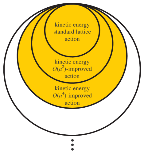
Figure 1: Suppression of finite cutoff errors by introducing improved actions for the nucleon kinetic energy.

Similarly, the interactions in the continuum limit can be organized in the chiral expansion as leading order, next-to-leading order, etc. But again for a chosen chiral order we may wish to include additional improvements to the interactions which reduce the finite cutoff errors. In this analysis we start by considering the simple LO lattice action without improvement, as shown in Figure 2. We note that the diagram shown is a bit simplistic since the improvement terms may in general include corrections for effects at nonzero lattice spacing such as broken Galilean invariance, etc.

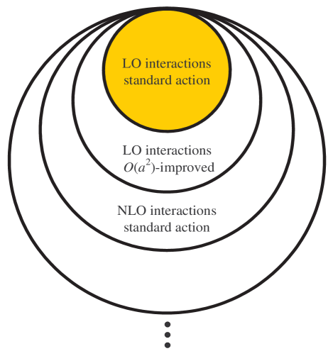
Figure 2: Hierarchy of interactions according to chiral order as well as improvements to each order due to nonzero lattice spacing.

Throughout our discussion we consider both the path integral formalism and the transfer matrix formalism.  The path integral formalism is useful for deriving the lattice Feynman rules and auxiliary field formulations, while the transfer matrix is used for the Monte Carlo simulations of light nuclei.  We start with the path integral formalism.  Let $\mathcal{Z}_{\bar{N}N}$ be the lattice partition function for free nucleons

$$\mathcal{Z}_{\bar{N}N}\propto\int DcDc^{\ast}\exp\left[-S_{\bar{N}N}\left(c,c^{\ast}\right)\right],$$ (7)

where

$$DcDc^{\ast}=\prod_{\vec{n},i,j}dc_{i,j}(\vec{n})dc_{i,j}^{\ast}(\vec{n}).$$ (8)

We use an $O(a^{4})$-improved lattice action with next-to-next-to-nearest neighbor hopping,

$$S_{\bar{N}N}(c,c^{\ast})= \sum_{\vec{n},i,j}\left[c_{i,j}^{\ast}(\vec{n})c_{i,j}(\vec{n}+\hat{0})+\left(-1+\frac{49h}{6}\right)c_{i,j}^{\ast}(\vec{n})c_{i,j}(\vec{n})\right]$$

$$-\frac{3h}{2}\sum_{\vec{n},l_{s},i,j}\left[c_{i,j}^{\ast}(\vec{n})c_{i,j}(\vec{n}+\hat{l}_{s})+c_{i,j}^{\ast}(\vec{n})c_{i,j}(\vec{n}-\hat{l}_{s})\right]$$

$$+\frac{3h}{20}\sum_{\vec{n},l_{s},i,j}\left[c_{i,j}^{\ast}(\vec{n})c_{i,j}(\vec{n}+2\hat{l}_{s})+c_{i,j}^{\ast}(\vec{n})c_{i,j}(\vec{n}-2\hat{l}_{s})\right]$$

$$-\frac{h}{90}\sum_{\vec{n},l_{s},i,j}\left[c_{i,j}^{\ast}(\vec{n})c_{i,j}(\vec{n}+3\hat{l}_{s})+c_{i,j}^{\ast}(\vec{n})c_{i,j}(\vec{n}-3\hat{l}_{s})\right].$$ (9)

We expect the $O(a^{4})$-improvement in the lattice dispersion relation to be useful when measuring scattering phase shifts on the lattice.

In this leading-order study we consider instantaneous one-pion exchange and no other interactions involving pions.  In our lattice formalism the pion field does not propagate in time and does not couple to physical pions.  This allows to avoid the problem of non-perturbative dynamical pion fields producing unrenormalized pion loops to all orders.  If at some point later on we wish to include interactions with physical low-energy pions we simply insert the corresponding operators with external pion fields.

The lattice action for free pions with purely instantaneous propagation is

$$S_{\pi\pi}(\pi_{I})=\alpha_{t}(\tfrac{m_{\pi}^{2}}{2}+3)\sum_{I=1,2,3}\sum_{\vec{n}}\pi_{I}(\vec{n})\pi_{I}(\vec{n})-\alpha_{t}\sum_{I=1,2,3}\sum_{\vec{n},l_{s}}\pi_{I}(\vec{n})\pi_{I}(\vec{n}+\hat{l}_{s}).$$ (10)

In order to simplify the Monte Carlo updating scheme later in our discussion it is helpful at this point to define a rescaled pion field,

$$\pi_{I}^{\prime}(\vec{n})=\sqrt{q_{\pi}}\pi_{I}(\vec{n}),$$ (11)

where

$$q_{\pi}=\alpha_{t}(m_{\pi}^{2}+6).$$ (12)

Then

$$S_{\pi\pi}(\pi_{I}^{\prime})=\frac{1}{2}\sum_{I=1,2,3}\sum_{\vec{n}}\pi_{I}^{\prime}(\vec{n})\pi_{I}^{\prime}(\vec{n})-\frac{\alpha_{t}}{q_{\pi}}\sum_{I=1,2,3}\sum_{\vec{n},l_{s}}\pi_{I}^{\prime}(\vec{n})\pi_{I}^{\prime}(\vec{n}+\hat{l}_{s}).$$ (13)

In momentum space the action is

$$S_{\pi\pi}(\pi_{I}^{\prime})=\frac{1}{L_{t}L^{3}}\sum_{I=1,2,3}\sum_{\vec{k}}\pi_{I}^{\prime}(-\vec{k})\pi_{I}^{\prime}(\vec{k})\left[\frac{1}{2}-\frac{\alpha_{t}}{q_{\pi}}\sum_{l_{s}}\cos\left(\tfrac{2\pi k_{l_{s}}}{L}\right)\right],$$ (14)

and so

$$\frac{\int D\pi_{I}^{\prime}\pi_{I}^{\prime}(\vec{n})\pi_{I}^{\prime}(\vec{0})\exp\left[-S_{\pi\pi}\right]}{\int D\pi_{I}^{\prime}\exp\left[-S_{\pi\pi}\right]}\text{ (no sum on }I\text{)}=\frac{1}{L_{t}L^{3}}\sum_{\vec{k}}e^{-i\frac{2\pi}{L_{t}}k_{t}\cdot n_{t}}e^{-i\frac{2\pi}{L}\vec{k}_{s}\cdot\vec{n}_{s}}D_{\pi}(\vec{k}_{s}),$$ (15)

where the pion propagator is

$$D_{\pi}(\vec{k}_{s})=\frac{1}{1-\tfrac{2\alpha_{t}}{q_{\pi}}\sum\limits_{l_{s}=1,2,3}\cos\left(\tfrac{2\pi k_{l_{s}}}{L}\right)}.$$ (16)

The pion correlation function at spatial separation $\vec{n}_{s}$ is then

$$\left\langle\pi_{I}^{\prime}(\vec{n}_{s})\pi_{I}^{\prime}(\vec{0})\right\rangle =\frac{\int D\pi_{I}^{\prime}\pi_{I}^{\prime}(\vec{n}_{s})\pi_{I}^{\prime}(\vec{0})\exp\left[-S_{\pi\pi}\right]}{\int D\pi_{I}^{\prime}\exp\left[-S_{\pi\pi}\right]}\text{ (no sum on }I\text{)}$$

$$=\frac{1}{L^{3}}\sum_{\vec{k}_{s}}e^{-i\frac{2\pi}{L}\vec{k}_{s}\cdot\vec{n}_{s}}D_{\pi}(\vec{k}_{s}).$$ (17)

V Pion-nucleon coupling

There are various ways to introduce spatial derivatives of the pion field on the lattice.  The simplest definition for the gradient of $\pi_{I}^{\prime}$ is to define a forward-backward lattice derivative.  For example we can write

$$\partial_{1}\pi_{I}^{\prime}(\vec{n})=\frac{1}{2}\left[\pi_{I}^{\prime}(\vec{n}+\hat{1})-\pi_{I}^{\prime}(\vec{n}-\hat{1})\right].$$ (18)

This is the method used in Lee et al. (2004).  The disadvantage is that it is a coarse derivative involving a separation distance of two lattice units.  We can avoid this if we think of the pion lattice points as being shifted by $-1/2$ lattice unit from the nucleon lattice points in each of the three spatial directions.  For each nucleon lattice point $\vec{n}_{\text{nucleon}}$ we associate a pion lattice point $\vec{n}_{\text{pion}}$,

$$\vec{n}_{\text{pion}}=\vec{n}_{\text{nucleon}}-\frac{1}{2}\hat{1}-\frac{1}{2}\hat{2}-\frac{1}{2}\hat{3}.$$ (19)

Then we have eight pion lattice points forming a cube centered at $\vec{n}_{\text{nucleon}}$,

$$\vec{n}_{\text{pion}},\quad\vec{n}_{\text{pion}}+\hat{1},\quad\vec{n}_{\text{pion}}+\hat{2},\quad\vec{n}_{\text{pion}}+\hat{3},$$

$$\vec{n}_{\text{pion}}+\hat{1}+\hat{2},\quad\vec{n}_{\text{pion}}+\hat{2}+\hat{3},\quad\vec{n}_{\text{pion}}+\hat{3}+\hat{1},\quad\vec{n}_{\text{pion}}+\hat{1}+\hat{2}+\hat{3}.$$ (20)

We use the same lattice vector notation $\vec{n}$ for both nucleons and pions.  However for nucleon fields and auxiliary fields to be introduced later $\vec{n}$ represents $\vec{n}_{\text{nucleon}}$ while for pion fields $\vec{n}$ refers to $\vec{n}_{\text{pion}}.$

The eight vertices of the pion cube in (20) can be used to define spatial derivatives of the pion field.  For each spatial direction $S=1,2,3$ we have

$$\Delta_{S}\pi_{I}^{\prime}(\vec{n})=\frac{1}{4}\sum_{\begin{subarray}{c}\nu_{1},\nu_{2},\nu_{3}=0,1\end{subarray}}(-1)^{\nu_{S}+1}\pi_{I}^{\prime}(\vec{n}+\vec{\nu}),\qquad\vec{\nu}=\nu_{1}\hat{1}+\nu_{2}\hat{2}+\nu_{3}\hat{3}.$$ (21)

The lattice pion-nucleon coupling in our lattice action is

$$S_{\pi\bar{N}N}(\pi_{I}^{\prime},c,c^{\ast})=\tfrac{g_{A}\alpha_{t}}{2f_{\pi}\sqrt{q_{\pi}}}{\displaystyle\sum_{S,I=1,2,3}}\Delta_{S}\pi_{I}^{\prime}(\vec{n})\rho_{S,I}(\vec{n}),$$ (22)

where $\rho_{S,I}(\vec{n})$ is the spin-isospin density,

$$\rho_{S,I}(\vec{n})=\sum_{i,j,i^{\prime},j^{\prime}=0,1}c_{i,j}^{\ast}(\vec{n})\left[\sigma_{S}\right]_{ii^{\prime}}\left[\tau_{I}\right]_{jj^{\prime}}c_{i^{\prime},j^{\prime}}(\vec{n}).$$ (23)

VI S-wave contact interactions

There are two S-wave contact interactions at lowest order.  Following Lee (2004) we choose the form

$$S_{\bar{N}N\bar{N}N}(c,c^{\ast})=\frac{C\alpha_{t}}{2}\sum_{\vec{n}}\left[\rho(\vec{n})\right]^{2}+\frac{C_{I}\alpha_{t}}{2}\sum_{I=1,2,3}\sum_{\vec{n}}\left[\rho_{I}(\vec{n})\right]^{2},$$ (24)

where $\rho(\vec{n})$ and $\rho_{I}(\vec{n})$ are the $SU(4)$-symmetric and isospin densities respectively,

$$\rho(\vec{n})=\sum_{i,j=0,1}c_{i,j}^{\ast}(\vec{n})c_{i,j}(\vec{n}),$$ (25)

$$\rho_{I}(\vec{n})=\sum_{i,j,j^{\prime}=0,1}c_{i,j}^{\ast}(\vec{n})\left[\tau_{I}\right]_{jj^{\prime}}c_{i,j^{\prime}}(\vec{n}).$$ (26)

Since the isospin singlet channel is more strongly attractive than the isospin triplet channel, we anticipate the signs for these coefficients to be $C<0$ and $C_{I}>0$. This will be confirmed in Sec. VIII, where the two-nucleon system is studied in detail.  As noted above, these can be written in terms of the more familiar coefficients $C_{S}$ and $C_{T}$ using the identity

$$C=C_{S}-2C_{T},\qquad C_{I}=-C_{T}.$$ (27)

We can use the Gaussian integral identities

$$\exp\left\{-\frac{C\alpha_{t}}{2}\left[\rho(\vec{n})\right]^{2}\right\}=\frac{1}{\sqrt{2\pi}}\int_{-\infty}^{\infty}ds\exp\left[-\frac{1}{2}s^{2}+\sqrt{-C\alpha_{t}}\rho(\vec{n})\cdot s\right],$$ (28)

and

$$\exp\left\{-\frac{C_{I}\alpha_{t}}{2}\sum_{I=1,2,3}\left[\rho_{I}(\vec{n})\right]^{2}\right\}$$

$$=\int\left(\prod\limits_{I=1,2,3}\frac{ds_{I}}{\sqrt{2\pi}}\right)\exp\left[-\frac{1}{2}\sum_{I=1,2,3}\left(s_{I}\right)^{2}+i\sqrt{C_{I}\alpha_{t}}\sum_{I=1,2,3}\rho_{I}(\vec{n})\cdot s_{I}\right].$$ (29)

Let us define the auxiliary field actions,

$$S_{ss}(s,s_{I})=\frac{1}{2}\sum_{\vec{n}}s^{2}(\vec{n})+\frac{1}{2}\sum_{I=1,2,3}\sum_{\vec{n}}\left[s_{I}(\vec{n})\right]^{2},$$ (30)

$$S_{s\bar{N}N}(s,s_{I},c,c^{\ast})=-\sqrt{-C\alpha_{t}}\sum_{\vec{n}}s(\vec{n})\rho(\vec{n})-i\sqrt{C_{I}\alpha_{t}}\sum_{I=1,2,3}\sum_{\vec{n}}s_{I}(\vec{n})\rho_{I}(\vec{n}).$$ (31)

Then we have

$$\int DsDs_{I}\;\exp\left[-S_{ss}(s,s_{I})-S_{s\bar{N}N}(s,s_{I},c,c^{\ast})\right]\propto\exp\left[-S_{\bar{N}N\bar{N}N}(c,c^{\ast})\right],$$ (32)

where

$$DsDs_{I}=\prod_{\vec{n},I}ds(\vec{n})ds_{I}(\vec{n}).$$ (33)

If we put all the pieces together the full path integral action at leading order is

$$\mathcal{Z}_{LO}\propto{\displaystyle\int}DcDc^{\ast}D\pi_{I}^{\prime}DsDs_{I}\exp\left[-S_{LO}(c,c^{\ast},\pi_{I}^{\prime},s,s_{I})\right],$$ (34)

where

$$S_{LO}=S_{\bar{N}N}+S_{\pi\pi}+S_{\pi\bar{N}N}+S_{ss}+S_{s\bar{N}N}.$$ (35)

VII Transfer matrix with auxiliary fields

The transfer matrix is the analog at nonzero temporal lattice spacing of the operator $\exp\left(-H\Delta t\right)$.  In order to derive the transfer matrix corresponding with the path integral action $S_{LO}$ we use the correspondence Creutz (1988, 2000)

$${\rm Tr}\left\{\colon F_{L_{t}-1}\left[a_{i^{\prime},j^{\prime}}^{\dagger}(\vec{n}_{s}^{\prime}),a_{i,j}(\vec{n}_{s})\right]\colon\times\cdots\times\colon F_{0}\left[a_{i^{\prime},j^{\prime}}^{\dagger}(\vec{n}_{s}^{\prime}),a_{i,j}(\vec{n}_{s})\right]\colon\right\}$$

$$=\int DcDc^{\ast}\exp\left\{\sum_{n_{t}=0}^{L_{t}-1}\sum_{\vec{n}_{s},i,j}c_{i,j}^{\ast}(\vec{n}_{s},n_{t})\left[c_{i,j}(\vec{n}_{s},n_{t})-c_{i,j}(\vec{n}_{s},n_{t}+1)\right]\right\}$$

$$\qquad\qquad\qquad\times\prod_{n_{t}=0}^{L_{t}-1}F_{n_{t}}\left[c_{i^{\prime},j^{\prime}}^{\ast}(\vec{n}_{s}^{\prime},n_{t}),c_{i,j}(\vec{n}_{s},n_{t})\right],$$ (36)

for general functions $F_{i}$ and antiperiodic boundary conditions in the time direction, $c_{i,j}(\vec{n}_{s},L_{t})=-c_{i,j}(\vec{n}_{s},0).$  The $\colon\colon$ symbols in (36) denote normal ordering.  Let us define the $SU(4)$-symmetric, isospin, and spin-isospin densities written in terms of creation and annihilation operators,

$$\rho^{a^{\dagger},a}(\vec{n}_{s})=\sum_{i,j=0,1}a_{i,j}^{\dagger}(\vec{n}_{s})a_{i,j}(\vec{n}_{s}),$$ (37)

$$\rho_{I}^{a^{\dagger},a}(\vec{n}_{s})=\sum_{i,j,j^{\prime}=0,1}a_{i,j}^{\dagger}(\vec{n}_{s})\left[\tau_{I}\right]_{jj^{\prime}}a_{i,j^{\prime}}(\vec{n}_{s}),$$ (38)

$$\rho_{S,I}^{a^{\dagger},a}(\vec{n}_{s})=\sum_{i,j,i^{\prime},j^{\prime}=0,1}a_{i,j}^{\dagger}(\vec{n}_{s})\left[\sigma_{S}\right]_{ii^{\prime}}\left[\tau_{I}\right]_{jj^{\prime}}a_{i^{\prime},j^{\prime}}(\vec{n}_{s}).$$ (39)

We also define the $O(a^{4})$-improved free nucleon lattice Hamiltonian

$$H_{\text{free}} =\frac{49}{12m}\sum_{\vec{n}_{s},i,j}a_{i,j}^{\dagger}(\vec{n}_{s})a_{i,j}(\vec{n}_{s})$$

$$-\frac{3}{4m}\sum_{\vec{n}_{s},l_{s},i,j}\left[a_{i,j}^{\dagger}(\vec{n}_{s})a_{i,j}(\vec{n}_{s}+\hat{l}_{s})+a_{i,j}^{\dagger}(\vec{n}_{s})a_{i,j}(\vec{n}_{s}-\hat{l}_{s})\right]$$

$$+\frac{1}{40m}\sum_{\vec{n}_{s},l_{s},i,j}\left[a_{i,j}^{\dagger}(\vec{n}_{s})a_{i,j}(\vec{n}_{s}+2\hat{l}_{s})+a_{i,j}^{\dagger}(\vec{n}_{s})a_{i,j}(\vec{n}_{s}-2\hat{l}_{s})\right]$$

$$-\frac{1}{180m}\sum_{\vec{n}_{s},l_{s},i,j}\left[a_{i,j}^{\dagger}(\vec{n}_{s})a_{i,j}(\vec{n}_{s}+3\hat{l}_{s})+a_{i,j}^{\dagger}(\vec{n}_{s})a_{i,j}(\vec{n}_{s}-3\hat{l}_{s})\right].$$ (40)

Using (36) the path integral with auxiliary fields can be expressed in the transfer matrix formalism as

$$\mathcal{Z}_{LO}\propto{\displaystyle\int}D\pi_{I}^{\prime}DsDs_{I}\;\exp\left[-S_{\pi\pi}-S_{ss}\right]\times Tr\left\{M^{(L_{t}-1)}(\pi_{I}^{\prime},s,s_{I})\times\cdots\times M^{(0)}(\pi_{I}^{\prime},s,s_{I})\right\},$$ (41)

where

$$M^{(n_{t})}(\pi_{I}^{\prime},s,s_{I})=\ \colon\exp\left\{-H_{\text{free}}\alpha_{t}-\tfrac{g_{A}\alpha_{t}}{2f_{\pi}\sqrt{q_{\pi}}}{\displaystyle\sum_{S,I}}\Delta_{S}\pi_{I}^{\prime}(\vec{n}_{s},n_{t})\rho_{S,I}^{a^{{\dagger}},a}(\vec{n}_{s})\right.$$

$$\left.\qquad+\sqrt{-C\alpha_{t}}\sum_{\vec{n}_{s}}s(\vec{n}_{s},n_{t})\rho^{a^{{\dagger}},a}(\vec{n}_{s})+i\sqrt{C_{I}\alpha_{t}}\sum_{I}\sum_{\vec{n}_{s}}s_{I}(\vec{n}_{s},n_{t})\rho_{I}^{a^{{\dagger}},a}(\vec{n}_{s})\right\}\colon.$$ (42)

VIII The two-nucleon system

For the two-nucleon system the entire linear space is small enough for typical lattice volumes that we can find the low-energy eigenstates on the lattice using iterative sparse matrix eigenvector methods such as the Lanczos method Lanczos (1950).  To do this calculation we construct the transfer matrix with only nucleon fields.  It is convenient to define

$$G_{S_{1}S_{2}}(\vec{n}_{s}) =\frac{\int D\pi_{I}^{\prime}\Delta_{S_{1}}\pi_{I}^{\prime}(\vec{n}_{s})\Delta_{S_{2}}\pi_{I}^{\prime}(0)\exp\left[-S_{\pi\pi}\right]}{\int D\pi_{I}^{\prime}\exp\left[-S_{\pi\pi}\right]}\text{ (no sum on }I\text{)}$$

$$=\frac{1}{16}\sum_{\nu_{1},\nu_{2},\nu_{3}=0,1}\sum_{\nu_{1}^{\prime},\nu_{2}^{\prime},\nu_{3}^{\prime}=0,1}(-1)^{\nu_{S_{1}}}(-1)^{\nu_{S_{2}}^{\prime}}\left\langle\pi_{I}^{\prime}(\vec{n}_{s}+\vec{\nu}-\vec{\nu}^{\prime})\pi_{I}^{\prime}(\vec{0})\right\rangle.$$ (43)

The path integral can now be written as

$$\mathcal{Z}_{LO}\propto{\rm Tr}\left\{M^{(L_{t}-1)}\times\cdots\times M^{(0)}\right\},$$ (44)

where

$$M^{(n_{t})} = \ \colon\exp\left\{-H_{\text{free}}\alpha_{t}-\frac{1}{2}C\alpha_{t}\sum_{\vec{n}_{s}}\left[\rho^{a^{{\dagger}},a}(\vec{n}_{s})\right]^{2}-\frac{1}{2}C_{I}\alpha_{t}\sum_{I}\sum_{\vec{n}_{s}}\left[\rho_{I}^{a^{{\dagger}},a}(\vec{n}_{s})\right]^{2}\right.$$ (45)

$$\qquad\qquad\left.+\tfrac{g_{A}^{2}\alpha_{t}^{2}}{8f_{\pi}^{2}q_{\pi}}\sum_{\begin{subarray}{c}S_{1},S_{2},I\end{subarray}}\sum_{\vec{n}_{s,1},\vec{n}_{s,2}}G_{S_{1}S_{2}}(\vec{n}_{s,1}-\vec{n}_{s,2})\rho_{S_{1},I}^{a^{{\dagger}},a}(\vec{n}_{s,1})\rho_{S_{2},I}^{a^{{\dagger}},a}(\vec{n}_{s,2})\right\}\colon.$$

We now calculate the two-nucleon spectrum in a periodic cube of length $L$ and use this information to determine the contact interaction coefficients $C$ and $C_{I}$.  We make use of Lüscher’s formula Lüscher (1986); Beane et al. (2004); Seki and van Kolck (2006) which relates the two-particle energy levels in a periodic cube of length $L$ to the S-wave phase shift,

$$p\cot\delta_{0}(p)=\frac{1}{\pi L}S\left(\eta\right),\qquad\eta=\left(\frac{Lp}{2\pi}\right)^{2},$$ (46)

where $S(\eta)$ is the three-dimensional zeta function,

$$S(\eta)=\lim_{\Lambda\rightarrow\infty}\left[\sum_{\vec{n}}\frac{\theta(\Lambda^{2}-\vec{n}^{2})}{\vec{n}^{2}-\eta}-4\pi\Lambda\right].$$ (47)

For $\left|\eta\right|<1$ we can expand in powers of $\eta$,

$$S(\eta) =-\frac{1}{\eta}+\lim_{\Lambda\rightarrow\infty}\left[\sum_{\vec{n}\neq\vec{0}}\frac{\theta(\Lambda^{2}-\vec{n}^{2})}{\vec{n}^{2}-\eta}-4\pi\Lambda\right]$$ (48)

$$=-\frac{1}{\eta}+S_{0}+S_{1}\eta^{1}+S_{2}\eta^{2}+S_{3}\eta^{3}\cdots,$$ (49)

where

$$S_{0}=\lim_{\Lambda\rightarrow\infty}\left[\sum_{\vec{n}\neq\vec{0}}\frac{\theta(\Lambda^{2}-\vec{n}^{2})}{\vec{n}^{2}}-4\pi\Lambda\right],$$ (50)

$$S_{j}=\sum_{\vec{n}\neq\vec{0}}\frac{1}{\left(\vec{n}^{2}\right)^{j+1}}\qquad j\geq 1.$$ (51)

The first few coefficients are

$$S_{0} =-8.913631,\quad S_{1}=16.532288,\quad S_{2}=8.401924,\quad S_{3}=6.945808,$$

$$S_{4} =6.426119,\quad S_{5}=6.202149,\quad S_{6}=6.098184,\quad S_{7}=6.048263.$$ (52)

Lüscher’s formula does not include cutoff effects or the contribution from coupled higher partial waves for particles with spin.  However we can neglect such corrections at asymptotically small momenta.  For small momenta we have the effective range expansion,

$$p\cot\delta_{0}(p)\approx-\frac{1}{a_{\text{scatt}}}+\frac{1}{2}r_{0}p^{2}+\cdots\text{,}$$ (53)

where $a_{\text{scatt}}$ is the scattering length and $r_{0}$ is the effective range.  In terms of $\eta$, the energy of the two-body scattering state is

$$E=\frac{p^{2}}{m}=\frac{\eta}{m}\left(\frac{2\pi}{L}\right)^{2}.$$ (54)

$S$ is an analytic function of $\eta$ near $\eta=0$, and so we can consider both $E<0$ and $E>0$.  We decouple the spin-singlet and spin-triplet contact interactions by expressing $C$ and $C_{I}$ as a linear combination of coefficients $C_{{}^{1}S_{0}}$ and $C_{{}^{3}S_{1}}$,

$$C =\left(3C_{{}^{1}S_{0}}+C_{{}^{3}S_{1}}\right)/4,$$ (55)

$$C_{I} =\left(C_{{}^{1}S_{0}}-C_{{}^{3}S_{1}}\right)/4.$$ (56)

The value of $C_{{}^{3}S_{1}}$ is tuned to give the physical deuteron binding energy, $-2.224575(9)$ MeV.  The value of $C_{{}^{1}S_{0}}$ is tuned using Lüscher’s formula to give the physical ${}^{1}S_{0}$ scattering length, $-23.76(1)$ fm.

At leading order in the two-nucleon system we expect finite cutoff errors to scale roughly as $O(\Lambda^{-1})$ or $O(a)$.  On the lattice we can relate this cutoff error to the probability that both nucleons occupy the same lattice site.  This localized two-nucleon state has a large positive expectation value for the kinetic energy and a large negative expectation value for the potential energy.  Let $E_{2}^{\text{localized}}$ be the expectation value of the total energy.  $E_{2}^{\text{localized}}$ need not be small compared with the cutoff energy $\Lambda^{2}/(2m)$.  Therefore transfer matrix elements involving this state may have a significant dependence on the temporal lattice spacing even for $a_{t}^{-1}$ as large as the cutoff energy.  This dependence shows up clearly in the $O(\Lambda^{-1})$ cutoff error, and we see the effect in the following results.

For $a=(100$ MeV$)^{-1}$ and $a_{t}=(70$ MeV$)^{-1},(200$ MeV$)^{-1},(10000$ MeV$)^{-1}$ we set the coefficients $C_{{}^{3}S_{1}}$ and $C_{{}^{1}S_{0}}$ using Lüscher’s formula.  We also use Lüscher’s formula to determine the effective range for the ${}^{1}S_{0}$ partial wave and both the scattering length and effective range for the ${}^{3}S_{1}$ partial wave.  The results are shown in Table 1.

$$\genfrac{}{}{0.0pt}{}{\text{Table 1: \ Coefficients and S-wave parameters for }a=(100\text{ MeV})^{-1}}{\begin{tabular}[c]{|c|c|c|c|c|c|}\hline\cr&$C_{{}^{3}S_{1}}$ (MeV${}^{-2}$)&$C_{{}^{1}S_{0}}$ (MeV${}^{-2}$)&$r_{0}^{{}^{1}S_{0}}$ (fm)&$a_{\text{scatt}}^{{}^{3}S_{1}}$ (fm)&$r_{0}^{{}^{3}S_{1}}$ (fm)\\ \hline\cr$a_{t}=(70$ MeV$)^{-1}$&$-5.714\times 10^{-5}$&$-5.021\times 10^{-5}$&$-0.179(7)$&$4.153(5)$&$-0.48(2)$\\ \hline\cr$a_{t}=(200$ MeV$)^{-1}$&$-6.706\times 10^{-5}$&$-5.794\times 10^{-5}$&$0.71(2)$&$4.522(1)$&$0.30(2)$\\ \hline\cr$a_{t}=(10000$ MeV$)^{-1}$&$-7.151\times 10^{-5}$&$-6.126\times 10^{-5}$&$1.03(2)$&$4.664(1)$&$0.53(2)$\\ \hline\cr experiment&$-$&$-$&$2.75(5)$&$5.424(4)$&$1.759(5)$\\ \hline\cr\end{tabular}}$$

Note that the values for $C_{{}^{1}S_{0}}$ and $C_{{}^{3}S_{1}}$ are reasonably close to the ones found at NLO and NNLO in the continuum formulation Epelbaum et al. (2002b). Also, within the pionless framework both values should be identical in the Wigner symmetry limit. The errorbars on the lattice data in Table 1 are error estimates from the least squares fit.  Since we work at leading order we do not expect agreement with the experimental values for the effective ranges.  However it is interesting to note that the effective ranges are actually negative for the largest temporal lattice spacing.  In the following we explain how this happens.

For some small fixed Euclidean time interval $\Delta t$ consider all transition amplitudes between two-nucleon states.  If $a_{t}\ll\Delta t$ then there are many temporal lattice steps in the time interval $\Delta t$.  Any transition amplitude involving states with two nucleons close together is enhanced to some degree by the negative potential energy of the delta function potential.  On the other hand if $a_{t}=\Delta t$ then there is only one temporal lattice step.  In this case only the forward matrix element for incoming and outgoing localized two-nucleon states is enhanced by the delta function potential.  This produces a sharp central peak in the two-nucleon wavefunction where the nucleons overlap and explains the decrease in effective range.  By the same reasoning we also expect a smaller value for the deuteron root-mean-square radius $r_{d}$.  In Table 2 we show results for $r_{d}$ and the deuteron quadrupole moment, $Q_{d}$, along with corresponding experimental values.  The experimental value quoted for $r_{d}$ is for the point proton root-mean-square radius.

at=(70 MeV)−11.566(1)0.144(1)at=(200 MeV)−11.668(1)0.171(1)at=(10000 MeV)−11.736(1)0.179(1)experiment1.9671(6)0.2859(3)FRACOPTable 2:  Properties of the deuteron for 𝑎superscript100 MeV1fragments fragmentsa𝑡(70 MeV)1fragments1.566(1)fragments0.144(1)fragmentsa𝑡(200 MeV)1fragments1.668(1)fragments0.171(1)fragmentsa𝑡(10000 MeV)1fragments1.736(1)fragments0.179(1)experimentfragments1.9671(6)fragments0.2859(3)\genfrac{}{}{0.0pt}{}{\text{Table 2: \ Properties of the deuteron for }a=(100\text{ MeV})^{-1}}{\begin{tabular}[c]{|c|c|c|}\hline\cr&$r_{d}$ (fm)&$Q_{d}$ (fm${}^{2}$)\\ \hline\cr$a_{t}=(70$ MeV$)^{-1}$&$1.566(1)$&$0.144(1)$\\ \hline\cr$a_{t}=(200$ MeV$)^{-1}$&$1.668(1)$&$0.171(1)$\\ \hline\cr$a_{t}=(10000$ MeV$)^{-1}$&$1.736(1)$&$0.179(1)$\\ \hline\cr experiment&$1.9671(6)$&$0.2859(3)$\\ \hline\cr\end{tabular}}

rd (fm) Qd (fm²) rd (fm) Qd (fm²)

As expected the root-mean-square radius of the deuteron is smaller than the physical value, and the deviation is greater for larger values of $a_{t}$.  The smaller radius also results in a substantial reduction in the quadrupole moment.

IX Zero-range clustering instability

We have found that the deuteron wavefunction at leading order shows some deficiencies which presumably get fixed at higher order in chiral effective field theory.  But since we now have in hand the coefficients of the leading-order contact interactions for lattice spacing $a=(100$ MeV$)^{-1}$ and $a_{t}=(70$ MeV$)^{-1},(200$ MeV$)^{-1},(10000$ MeV$)^{-1}$, we can consider systems with more than two nucleons at leading order in chiral effective field theory.  Unfortunately here we find more problems.  In the helium-4 system we discover that the ground state is severely overbound and consists almost entirely of the quantum state with all four nucleons occupying the same lattice site.  This clustering instability can be understood as the result of two contributing factors.  The first is that chiral effective field theory at leading order gives a poor description of S-wave scattering above a center of mass momentum of $50$ MeV.  The leading-order contact interactions are momentum independent and, as a result, are too strong at high momenta.  The second is a combinatorial enhancement of the contact interactions when more than two nucleons occupy the same lattice site.  This effect has been studied in two-dimensional large-$N$ droplets with zero-range attraction Lee (2006a).  Similar effects have also been considered in systems of higher-spin fermions in optical traps and lattices Wu et al. (2003); Wu (2005).  To illustrate we briefly discuss how the problem arises in $SU(4)$-symmetric pionless theory at leading order using a Hamiltonian lattice formalism.

Let $E_{1}^{\text{localized}}$ be the expectation value for the kinetic energy of a single nucleon localized on a single lattice site and let $V_{2}<0$ be the potential energy between two nucleons on the same lattice site.  If we fix the two-particle scattering length then both $E_{1}^{\text{localized}}$ and $V_{2}$ scale linearly with the cutoff energy,

$$E_{1}^{\text{localized}}\sim-V_{2}\sim\frac{\Lambda^{2}}{2m},\qquad\Lambda=\pi a^{-1}.$$ (57)

A detailed calculation of $V_{2}$ for infinite scattering length can be found in Lee and Schäfer (2006).  The total energies associated with putting two, three, or four nucleons on the same lattice site are

$$E_{2}^{\text{localized}} =2E_{1}^{\text{localized}}+V_{2},$$ (58)

$$E_{3}^{\text{localized}} =3E_{1}^{\text{localized}}+3V_{2},$$ (59)

$$E_{4}^{\text{localized}} =4E_{1}^{\text{localized}}+6V_{2}.$$ (60)

An instability forms as we increase $A$ because the kinetic energy scales as the number of nucleons, $A,$ while the potential energy scales as $\binom{A}{2}$.  Of course the Pauli exclusion principle prevents more than four nucleons from sitting on the same lattice site, and so the problem is most severe in the four-nucleon system.

In the leading-order pionless theory it has been shown that $V_{2}<-E_{1}^{\text{localized}}$ Lee and Schäfer (2006).  Therefore $E_{3}^{\text{localized}}$ is negative and scales with the cutoff energy.  This produces an instability for the three-nucleon system in the absence of three-body forces or other stabilizing effects.  The instability of the triton for zero range forces was first studied by Thomas Thomas (1935).  There have been a number of more recent studies of the triton in pionless effective field theory as well as more general three-body systems with short range interactions and long scattering lengths Efimov (1971, 1993); Bedaque et al. (1999a, b); Bedaque et al. (2000); Braaten and Hammer (2006); Borasoy et al. (2006); Platter (2006).  It has also been shown that when the cutoff dependence in the three-nucleon system is removed using a three-nucleon contact interaction, then the binding energy of the four-nucleon system appears also to be cutoff independent Platter et al. (2004, 2005).  In our lattice Hamiltonian notation we denote $V_{3}$ as the potential energy associated with the three-nucleon contact interaction.  The new localized energies are then

$$E_{2}^{\text{localized}} =2E_{1}^{\text{localized}}+V_{2},$$ (61)

$$E_{3}^{\text{localized}} =3E_{1}^{\text{localized}}+3V_{2}+V_{3},$$ (62)

$$E_{4}^{\text{localized}} =4E_{1}^{\text{localized}}+6V_{2}+4V_{3}.$$ (63)

Clearly $E_{4}^{\text{localized}}$ would be stabilized by $4V_{3}$ for sufficiently large $V_{3}>0$.  However for realistic nuclear binding energies, it was found that the desired cutoff independence in helium-4 does not emerge until the cutoff momentum $\Lambda$ exceeds $8$ fm^-1 Platter et al. (2005).  Unfortunately this high cutoff momentum makes it a difficult starting point for lattice simulations of realistic light nuclei.  A cutoff momentum of $8$ fm^-1 corresponds with a lattice spacing of about $0.4$ fm.  From a computational standpoint this combination of short lattice spacing and strong repulsive forces makes lattice simulations nearly impossible due to sign and phase oscillations.  Given these difficulties we try a different approach.  We keep the lattice spacing large, $a\sim(100$ MeV$)^{-1}\sim 2$ fm, and again consider chiral effective field theory at leading order.  But this time we introduce higher-derivative operators which improve the S-wave scattering amplitude at higher momenta.  We expect that this should remove the clustering instability in the four-nucleon system.

X Higher-derivative terms

As explained in the previous section, the interactions at leading order with delta function contact interactions are too strong at large momenta. Their contribution would be appropriately weakened by interactions of higher chiral order. But a full investigation of higher order contributions is beyond the scope of this first exploratory study and is deferred to future work. Instead we consider here the effect of higher derivative terms which reduce cutoff errors by improving the delta function contact interaction. We fix the problem of clustering instability by introducing an ${\cal O}(a^{2})$-improved broadening for the leading contact interactions $C$ and $C_{I}$, as illustrated in Fig. 3. This is by no means a full NLO calculation, but rather an LO calculation with ${\cal O}(a^{2})$-improvement to reduce cutoff errors.

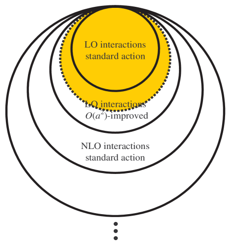
Figure 3: Suppression of finite cutoff errors by broadening the leading order contact interactions.

To this aim, we define the momentum-dependent densities,

$$\rho^{a^{{\dagger}},a}(\vec{q}_{s})=\sum_{\vec{n}_{s}}\rho^{a^{{\dagger}},a}(\vec{n}_{s})e^{i\vec{q}_{s}\cdot\vec{n}_{s}},$$ (64)

$$\rho_{I}^{a^{{\dagger}},a}(\vec{q}_{s})=\sum_{\vec{n}_{s}}\rho_{I}^{a^{{\dagger}},a}(\vec{n}_{s})e^{i\vec{q}_{s}\cdot\vec{n}_{s}},$$ (65)

where $\vec{q}_{s}$ is the spatial momentum on the lattice.  We can write $\vec{q}_{s}$ as

$$\vec{q}_{s}=\frac{2\pi}{L}\vec{k}_{s},$$ (66)

where the components of $\vec{k}_{s}$ are integers from $0$ to $L-1$.

The transfer matrix $M^{(n_{t})}$ with only nucleon fields was defined in (45).  The contact interactions in $M^{(n_{t})}$ have the form

$$-\frac{1}{2}C\alpha_{t}\sum_{\vec{n}_{s}}\left[\rho^{a^{{\dagger}},a}(\vec{n}_{s})\right]^{2}-\frac{1}{2}C_{I}\alpha_{t}\sum_{I=1,2,3}\sum_{\vec{n}_{s}}\left[\rho_{I}^{a^{{\dagger}},a}(\vec{n}_{s})\right]^{2}$$

$$=\frac{1}{L^{3}}\sum_{\vec{q}_{s}}\left[-\frac{1}{2}C\alpha_{t}\rho^{a^{{\dagger}},a}(\vec{q}_{s})\rho^{a^{{\dagger}},a}(-\vec{q}_{s})-\frac{1}{2}C_{I}\alpha_{t}\sum_{I=1,2,3}\rho_{I}^{a^{{\dagger}},a}(\vec{q}_{s})\rho_{I}^{a^{{\dagger}},a}(-\vec{q}_{s})\right].$$ (67)

We replace these by the momentum-dependent interactions,

$$\frac{1}{L^{3}}\sum_{\vec{q}_{s}}f(\vec{q}_{s}^{\ 2})\left[-\frac{1}{2}C\alpha_{t}\rho^{a^{{\dagger}},a}(\vec{q}_{s})\rho^{a^{{\dagger}},a}(-\vec{q}_{s})-\frac{1}{2}C_{I}\alpha_{t}\sum_{I=1,2,3}\rho_{I}^{a^{{\dagger}},a}(\vec{q}_{s})\rho_{I}^{a^{{\dagger}},a}(-\vec{q}_{s})\right],$$ (68)

where the coefficient function $f(\vec{q}_{s}^{\ 2})$ is defined as

$$f(\vec{q}_{s}^{\ 2})=f_{0}^{-1}\exp\left[-b{\displaystyle\sum\limits_{l_{s}=1,2,3}}\left(1-\cos q_{l_{s}}\right)\right],$$ (69)

and the normalization factor $f_{0}$ is determined by the condition

$$f_{0}=\frac{1}{L^{3}}\sum_{\vec{q}_{s}}\exp\left[-b{\displaystyle\sum\limits_{l_{s}=1,2,3}}\left(1-\cos q_{l_{s}}\right)\right].$$ (70)

The coefficient $b$ is determined at a later stage when we find the effective range.  For small $\vec{q}_{s}$ we see that $f(\vec{q}_{s}^{\ 2})$ reduces to a Gaussian form,

$$f(\vec{q}_{s}^{\ 2})\approx f_{0}^{-1}\exp\left(-\frac{b}{2}\vec{q}_{s}^{\ 2}\right).$$ (71)

We can introduce exactly the same momentum-dependent interactions in the transfer matrix formalism with auxiliary fields,

$$\mathcal{Z}_{LO}\propto{\displaystyle\int}D\pi_{I}^{\prime}DsDs_{I}\;\exp\left[-S_{\pi\pi}-S_{ss}\right]\times{\rm Tr}\left\{M^{(L_{t}-1)}(\pi_{I}^{\prime},s,s_{I})\times\cdots\times M^{(0)}(\pi_{I}^{\prime},s,s_{I})\right\}.$$ (72)

To do this we replace

$$S_{ss}=\frac{1}{2}\sum_{\vec{n}}s^{2}(\vec{n})+\frac{1}{2}\sum_{I}\sum_{\vec{n}}\left[s_{I}(\vec{n})\right]^{2}$$ (73)

by the nonlocal action

$$\frac{1}{2}\sum_{\vec{n}_{s},\vec{n}_{s}^{\prime},n_{t}}s(\vec{n}_{s},n_{t})f^{-1}(\vec{n}_{s}-\vec{n}_{s}^{\prime})s(\vec{n}_{s}^{\prime},n_{t})+\frac{1}{2}\sum_{I}\sum_{\vec{n}_{s},\vec{n}_{s}^{\prime},n_{t}}s_{I}(\vec{n}_{s},n_{t})f^{-1}(\vec{n}_{s}-\vec{n}_{s}^{\prime})s_{I}(\vec{n}_{s}^{\prime},n_{t}).$$ (74)

The function $f^{-1}$ is defined as

$$f^{-1}(\vec{n}_{s}-\vec{n}_{s}^{\prime})=\frac{1}{L^{3}}\sum_{\vec{q}_{s}}\frac{1}{f(\vec{q}_{s}^{\ 2})}e^{-i\vec{q}_{s}\cdot(\vec{n}_{s}-\vec{n}_{s}^{\prime})}.$$ (75)

When the auxiliary fields are integrated out we recover the momentum-dependent interactions in (68).

XI The two-nucleon system revisited

Using the new transfer matrix with momentum-dependent interactions we now revisit the two-nucleon system.  Just as before we set $C_{{}^{3}S_{1}}$ and $C_{{}^{1}S_{0}}$ to give the physical deuteron binding energy and physical ${}^{1}S_{0}$ scattering length.  We also tune the coefficient $b$ so that when $C_{{}^{3}S_{1}}$ and $C_{{}^{1}S_{0}}$ are determined, we also get the correct value for the average effective range $\frac{1}{2}\left(r_{0}^{{}^{1}S_{0}}+r_{0}^{{}^{3}S_{1}}\right).$  For $a=(100\ \mbox{MeV})^{-1}$ and $a_{t}=(70\ \mbox{MeV})^{-1}$ we find $C_{{}^{3}S_{1}}=-4.780\times 10^{-5}$ MeV^-2, $C_{{}^{1}S_{0}}=-3.414\times 10^{-5}$ MeV^-2, and $b=0.6$.  The new results are shown in Tables 3 and 4.

lattice3.20(1)5.30(1)1.46(3)experiment2.75(5)5.424(4)1.759(5)FRACOPTable 3: S-wave parametersfragments latticefragments3.20(1)fragments5.30(1)fragments1.46(3)experimentfragments2.75(5)fragments5.424(4)fragments1.759(5)\genfrac{}{}{0.0pt}{}{\text{Table 3: S-wave parameters}}{\begin{tabular}[c]{|c|c|c|c|}\hline\cr&$r_{0}^{{}^{1}S_{0}}$ (fm)&$a_{\text{scatt}}^{{}^{3}S_{1}}$ (fm)&$r_{0}^{{}^{3}S_{1}}$ (fm)\\ \hline\cr lattice&$3.20(1)$&$5.30(1)$&$1.46(3)$\\ \hline\cr experiment&$2.75(5)$&$5.424(4)$&$1.759(5)$\\ \hline\cr\end{tabular}}

r0S01 (fm) ascattS13 (fm) r0S13 (fm) r0S01 (fm) ascattS13 (fm) r0S13 (fm)

lattice1.989(1)0.278(1)experiment1.9671(6)0.2859(3)FRACOPTable 4:  Properties of the deuteronfragments latticefragments1.989(1)fragments0.278(1)experimentfragments1.9671(6)fragments0.2859(3)\genfrac{}{}{0.0pt}{}{\text{Table 4: \ Properties of the deuteron}}{\begin{tabular}[c]{|c|c|c|}\hline\cr&$r_{d}$ (fm)&$Q_{d}$ (fm${}^{2}$)\\ \hline\cr lattice&$1.989(1)$&$0.278(1)$\\ \hline\cr experiment&$1.9671(6)$&$0.2859(3)$\\ \hline\cr\end{tabular}}

rd (fm) Qd (fm²) rd (fm) Qd (fm²)

The agreement with experimental values is now good.  There is clear improvement over the earlier results shown in Tables 1 and 2.

We can probe the shape of deuteron wavefunction by computing the nucleon density correlation function

$$\left\langle:\rho^{a^{{\dagger}},a}(\vec{n}_{s})\rho^{a^{{\dagger}},a}(\vec{0}):\right\rangle.$$ (76)

If $A$ is the total number of nucleons then

$$A=\sum_{\vec{n}_{s}}\left\langle\rho^{a^{{\dagger}},a}(\vec{n}_{s})\right\rangle.$$ (77)

We also find

$$\sum_{\vec{n}_{s}}\left\langle:\rho^{a^{{\dagger}},a}(\vec{n}_{s})\rho^{a^{{\dagger}},a}(\vec{0}):\right\rangle =\sum_{\vec{n}_{s}}\left\langle\rho^{a^{{\dagger}},a}(\vec{n}_{s})\rho^{a^{{\dagger}},a}(\vec{0})\right\rangle-\left\langle\rho^{a^{{\dagger}},a}(\vec{0})\right\rangle$$

$$=L^{-3}\left(A^{2}-A\right).$$ (78)

Let us define the normalized density correlation function as

$$G_{\rho\rho}(\vec{n}_{s})=L^{3}\left(A^{2}-A\right)^{-1}\left\langle:\rho^{a^{{\dagger}},a}(\vec{n}_{s})\rho^{a^{{\dagger}},a}(\vec{0}):\right\rangle.$$ (79)

In Figure 4, we show $G_{\rho\rho}(\vec{n}_{s})$ for the deuteron in the $xy$-plane.  We have aligned the deuteron spin in the $+z$-direction.  Keeping the deuteron spin in the $+z$-direction, in Figure 5 we show $G_{\rho\rho}(\vec{n}_{s})$ in the $yz$-plane.  A small asymmetry can be seen between the $y$ and $z$ directions.  This is a signal of the deuteron quadrupole moment and can be seen more easily in Fig. 6, where we have taken an antisymmetric combination under interchange of $y$ and $z$ .

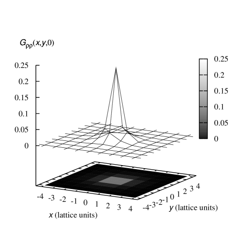
Figure 4: Density correlations in the $xy$-plane for a deuteron with spin in the $+z$-direction.

Figure 5: Density correlations in the $yz$-plane for a deuteron with spin in the $+z$-direction.

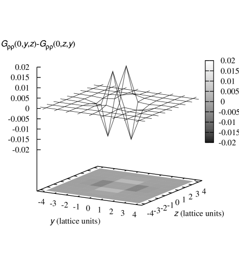
Figure 6: A linear combination of density correlations in the $yz$-plane that is antisymmetric under interchange of $y$ and $z$.  The deuteron spin points in the $+z$-direction.

XII Transfer matrix projection method for light nuclei

We simulate light nuclei by using the Monte Carlo transfer matrix projection method introduced in Lee (2006b).  Since this method may be unfamiliar, we first give an overview of the calculation using continuum notation before describing the details of the lattice transfer matrix calculation.

Let $\left|\Psi_{Z,N}^{\text{free}}\right\rangle$ be a Slater determinant of free particle standing waves in a periodic cube for $Z$ protons and $N$ neutrons.  We define $A=Z+N$ as the total number of nucleons.  Let $H_{LO}$ denote the Hamiltonian including instantaneous one-pion exchange and the improved higher-derivative contact interactions.  Let $H_{SU(4)\not\pi}$ be the same Hamiltonian but with both $C_{I}$ and $g_{A}$ set to zero.  As the notation suggests, $H_{SU(4)\not\pi}$ is invariant under $SU(4)$ Wigner symmetry.  Wigner symmetry refers to an idealized limit where spin and isospin degrees of freedom can be interchanged and the $SU(2)\times SU(2)$ spin-isospin symmetry is elevated to an $SU(4)$ symmetry.  Let us define a trial wavefunction

$$\left|\Psi(t^{\prime})\right\rangle=\exp\left[-H_{SU(4)\not\pi}t^{\prime}\right]\left|\Psi_{Z,N}^{\text{free}}\right\rangle.$$ (80)

With this trial wavefunction we define the amplitude,

$$Z(t)=\left\langle\Psi(t^{\prime})\right|\exp\left[-H_{LO}t\right]\left|\Psi(t^{\prime})\right\rangle,$$ (81)

as well as the transient energy,

$$E(t)=-\frac{\partial}{\partial t}\left[\ln Z(t)\right].$$ (82)

In limit of large $t$ we get

$$\lim_{t\rightarrow\infty}E(t)=E_{0},$$ (83)

where $E_{0}$ is the energy of the lowest eigenstate $\left|\Psi_{0}\right\rangle$ of $H_{LO}$ with a nonzero inner product with $\left|\Psi(t^{\prime})\right\rangle$.  In order to compute the expectation value of some normal-ordered operator $O$ we define

$$Z_{O}(t)=\left\langle\Psi(t^{\prime})\right|\exp\left[-H_{LO}t/2\right]\,O\,\exp\left[-H_{LO}t/2\right]\left|\Psi(t^{\prime})\right\rangle.$$ (84)

The expectation value of $O$ for $\left|\Psi_{0}\right\rangle$ can be computed in the large $t$ limit,

$$\lim_{t\rightarrow\infty}\frac{Z_{O}(t)}{Z(t)}=\left\langle\Psi_{0}\right|O\left|\Psi_{0}\right\rangle.$$ (85)

In this two-step approach we use $\exp\left[-H_{SU(4)\not\pi}t^{\prime}\right]$ as an approximate inexpensive low-energy filter and $\exp\left[-H_{LO}t\right]$ as an exact low-energy filter.  The projection $\exp\left[-H_{SU(4)\not\pi}t^{\prime}\right]$ is computationally inexpensive because the path integral for leading-order pionless effective field theory in the $SU(4)$ limit is strictly positive for any even number of nucleons Lee (2005); Chen et al. (2004).  Although there is no positivity theorem for odd numbers of nucleons, sign oscillations are also suppressed in odd systems because it is only one particle or one hole away from an even system with no sign oscillations.

In the lattice transfer matrix formalism we construct $\left|\Psi(t^{\prime})\right\rangle$ using

$$\left|\Psi(t^{\prime})\right\rangle={\displaystyle\int}Ds\;\exp\left[-S_{ss}(s)\right]\times M_{SU(4)\not\pi}^{(L_{t_{o}}-1)}(s)\times\cdots\times M_{SU(4)\not\pi}^{(0)}(s)\left|\Psi_{Z,N}^{\text{free}}\right\rangle,$$ (86)

where $t^{\prime}=L_{t_{o}}a_{t}$.  $M_{SU(4)\not\pi}^{(i)}(s)$ is the same as $M^{(i)}(\pi_{I}^{\prime},s,s_{I})$ except with $g_{A}=C_{I}=0$.  We have omitted the dependence on $\pi_{I}^{\prime}$ and $s_{I}$ since these completely decouple in the $SU(4)$ symmetric theory.  The amplitude $Z(t)$ is constructed using

$$Z(t)={\displaystyle\int}D\pi_{I}^{\prime}DsDs_{I}\;\exp\left[-S_{\pi\pi}-S_{ss}\right]\times\left\langle\Psi(t^{\prime})\right|M^{(L_{t_{i}}-1)}(\pi_{I}^{\prime},s,s_{I})\times\cdots\times M^{(0)}(\pi_{I}^{\prime},s,s_{I})\left|\Psi(t^{\prime})\right\rangle,$$ (87)

where $t=L_{t_{i}}a_{t}$.  In this case the full leading-order transfer matrix is used.  We compute $Z_{O}(t)$ by inserting the normal-ordered operator $O$ in the middle of the string of transfer matrices,

$$Z_{O}(t) ={\displaystyle\int}D\pi_{I}^{\prime}DsDs_{I}\;\exp\left[-S_{\pi\pi}-S_{ss}\right]\times\left\langle\Psi(t^{\prime})\right|M^{(L_{t_{i}}-1)}(\pi_{I}^{\prime},s,s_{I})\times\cdots$$

$$\qquad\qquad\cdots\times M^{(L_{t_{i}}/2)}(\pi_{I}^{\prime},s,s_{I})\,O\,M^{(L_{t_{i}}/2-1)}(\pi_{I}^{\prime},s,s_{I})\times\cdots\times M^{(0)}(\pi_{I}^{\prime},s,s_{I})\left|\Psi(t^{\prime})\right\rangle.$$ (88)

A schematic overview of the transfer matrix calculation is shown in Fig. 7.

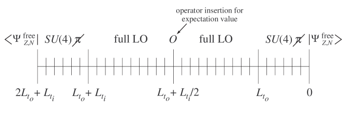
Figure 7: Overview of the various pieces of the transfer matrix calculation.

Let $\left|\psi_{1}\right\rangle,\cdots,\left|\psi_{A}\right\rangle$ be the free particle standing waves comprising $\left|\Psi_{Z,N}^{\text{free}}\right\rangle.$  We note that for the transfer matrices in the auxiliary field formalism there are no direct interactions between particles, only single-nucleon operators interacting with the background pion and auxiliary fields.  It is easier to see this fact if we pretend for the moment that each of the $A$ nucleons has an extra quantum number which makes them distinguishable.  Let us label the extra quantum number as $X$, where $X=1,\cdots,A.$  Then we have

$$a_{i,j}^{\dagger},a_{i,j}\rightarrow\left\{a_{i,j,X}^{\dagger},a_{i,j,X}\right\}_{X=1,\cdots,A}.$$ (89)

We use an $X$ subscript to indicate this replacement for creation and annihilation operators.  The transfer matrices $M_{SU(4)\not\pi}^{(n_{t})}$ and $M^{(n_{t})}$ factorize into transfer matrices for each $X$,

$$M_{SU(4)\not\pi}^{(n_{t})} \rightarrow{\displaystyle\prod\limits_{X=1,\cdots,A}}M_{SU(4)\not\pi,X}^{(n_{t})},$$ (90)

$$M^{(n_{t})} \rightarrow{\displaystyle\prod\limits_{X=1,\cdots,A}}M_{X}^{(n_{t})}.$$ (91)

So long as the initial and final state wavefunctions are completely antisymmetric in $X$, this error in quantum statistics has no effect on the final amplitude.  We can write the full $A$-nucleon transfer matrix element as a determinant of an $A\times A$ matrix of single-particle matrix elements,

$$\mathcal{M}_{ij}(\pi_{I}^{\prime},s,s_{I},t^{\prime},t) =\left\langle\psi_{i,X}\right|M_{SU(4)\not\pi,X}^{(2L_{t_{o}}+L_{t_{i}}-1)}\times\cdots\times M_{SU(4)\not\pi,X}^{(L_{t_{o}}+L_{t_{i}})}M_{X}^{(L_{t_{o}}+L_{t_{i}}-1)}\times\cdots$$

$$\cdots\times M_{X}^{(L_{t_{o}})}M_{SU(4)\not\pi,X}^{(L_{t_{o}}-1)}\times\cdots\times M_{SU(4)\not\pi,X}^{(0)}\left|\psi_{j,X}\right\rangle.$$ (92)

The indices $i,j$ go from $1$ to $A$.  The calculation of $Z(t)$ now reduces to computing

$$Z(t)={\displaystyle\int}D\pi_{I}^{\prime}DsDs_{I}\;\exp\left\{-S_{\pi\pi}-S_{ss}\right\}\det\mathcal{M}(\pi_{I}^{\prime},s,s_{I},t^{\prime},t).$$ (93)

There are many different ways to compute the amplitude $Z_{O}(t)$, and the most efficient method will depend on the operator $O$.  Insertions of an operator measuring spatial difermion pair correlations was discussed in Lee . Here we consider an operator that measures spatial correlations of the total nucleon density,

$$O=\ :\rho^{a^{{\dagger}},a}(\vec{n}_{s})\rho^{a^{{\dagger}},a}(\vec{0}):.$$ (94)

For this operator it is convenient to use the identity

$$O=\lim_{\epsilon_{1},\epsilon_{2}\rightarrow 0}\frac{\partial}{\partial\epsilon_{1}}\frac{\partial}{\partial\epsilon_{2}}M(\epsilon_{1},\epsilon_{2}),$$ (95)

where

$$M(\epsilon_{1},\epsilon_{2})=\ :\exp\left[\epsilon_{1}\sum_{i,j}a_{i,j}^{{\dagger}}(\vec{n}_{s})a_{i,j}(\vec{n}_{s})+\epsilon_{2}\sum_{i,j}a_{i,j}^{{\dagger}}(\vec{0})a_{i,j}(\vec{0})\right]:.$$ (96)

This is useful because $M(\epsilon_{1},\epsilon_{2})$ itself looks like a transfer matrix with only single-nucleon operators.  Let us define the new single-particle matrix elements,

$$\mathcal{M}_{ij}(\pi_{I}^{\prime},s,s_{I},t^{\prime},t,\epsilon_{1},\epsilon_{2})$$

$$=\left\langle\psi_{i,X}\right|M_{SU(4)\not\pi,X}^{(2L_{t_{o}}+L_{t_{i}}-1)}\times\cdots\times M_{SU(4)\not\pi,X}^{(L_{t_{o}}+L_{t_{i}})}M_{X}^{(L_{t_{o}}+L_{t_{i}}-1)}\times\cdots$$

$$\cdots\times M_{X}^{(L_{t_{o}}+L_{t_{i}}/2)}M_{X}(\epsilon_{1},\epsilon_{2})M_{X}^{(L_{t_{o}}+L_{t_{i}}/2-1)}\times\cdots\times M_{X}^{(L_{t_{o}})}M_{SU(4)\not\pi,X}^{(L_{t_{o}}-1)}\times\cdots\times M_{SU(4)\not\pi,X}^{(0)}\left|\psi_{j,X}\right\rangle.$$ (97)

We then find

$$Z_{O}(t)=\lim_{\epsilon_{1},\epsilon_{2}\rightarrow 0}\frac{\partial}{\partial\epsilon_{1}}\frac{\partial}{\partial\epsilon_{2}}{\displaystyle\int}D\pi_{I}^{\prime}DsDs_{I}\;\exp\left\{-S_{\pi\pi}-S_{ss}\right\}\det\mathcal{M}(\pi_{I}^{\prime},s,s_{I},t^{\prime},t,\epsilon_{1},\epsilon_{2}).$$ (98)

We use hybrid Monte Carlo to update the fields $\pi_{I}^{\prime},s,s_{I}$ Duane et al. (1987).  We introduce conjugate fields $p_{\pi_{I}^{\prime}},p_{s},p_{s_{I}}$ and use molecular dynamics trajectories to generate new configurations for $p_{\pi_{I}^{\prime}},p_{s},$ $p_{s_{I}},\pi_{I}^{\prime},s,s_{I}$ which keep

$$H_{HMC}=\frac{1}{2}\sum_{I,\vec{n}}p_{\pi_{I}^{\prime}}^{2}(\vec{n})+\frac{1}{2}\sum_{\vec{n}}p_{s}^{2}(\vec{n})+\frac{1}{2}\sum_{I,\vec{n}}p_{s_{I}}^{2}(\vec{n})+V(\pi_{I}^{\prime},s,s_{I})$$ (99)

constant, where

$$V(\pi_{I}^{\prime},s,s_{I})=S_{\pi\pi}+S_{ss}-\log\left\{\left|\det\mathcal{M}(\pi_{I}^{\prime},s,s_{I},t^{\prime},t_{\text{end}})\right|\right\}.$$ (100)

$t_{\text{end}}$ denotes the largest value of $t$ being considered.  Upon completion of each molecular dynamics trajectory, we apply a Metropolis accept or reject step for the new configuration according to the probability distribution $e^{-H_{HMC}}$.  This process of molecular dynamics trajectory and Metropolis step is repeated many times.  Each time for the current configuration$,\mathcal{C}$, we measure

$$e^{i\theta}(\mathcal{C})=\frac{\det\mathcal{M}(\pi_{I}^{\prime},s,s_{I},t^{\prime},t_{\text{end}})}{\left|\det\mathcal{M}(\pi_{I}^{\prime},s,s_{I},t^{\prime},t_{\text{end}})\right|},$$ (101)

$$Z(t,\mathcal{C})=\frac{\det\mathcal{M}(\pi_{I}^{\prime},s,s_{I},t^{\prime},t)}{\left|\det\mathcal{M}(\pi_{I}^{\prime},s,s_{I},t^{\prime},t_{\text{end}})\right|},$$ (102)

and

$$Z_{O}(\epsilon_{1},\epsilon_{2},\mathcal{C})=\frac{\det\mathcal{M}(\pi_{I}^{\prime},s,s_{I},t^{\prime},t_{\text{end}},\epsilon_{1},\epsilon_{2})}{\left|\det\mathcal{M}(\pi_{I}^{\prime},s,s_{I},t^{\prime},t_{\text{end}})\right|}.$$ (103)

We take the ensemble averages for each measurement and form the ratios

$$\frac{Z(t)}{Z(t_{\text{end}})}=\frac{\left\langle Z(t,\mathcal{C})\right\rangle}{\left\langle e^{i\theta}(\mathcal{C})\right\rangle},$$ (104)

and

$$\frac{Z_{O}(t_{\text{end}})}{Z(t_{\text{end}})}=\lim_{\epsilon_{1},\epsilon_{2}\rightarrow 0}\frac{\partial}{\partial\epsilon_{1}}\frac{\partial}{\partial\epsilon_{2}}\frac{\left\langle Z_{O}(\epsilon_{1},\epsilon_{2},\mathcal{C})\right\rangle}{\left\langle e^{i\theta}(\mathcal{C})\right\rangle}.$$ (105)

The ground state energy $E_{0}$ is extracted using

$$\lim_{t_{\text{end}}\rightarrow\infty}\frac{Z(t_{\text{end}}-\Delta t)}{Z(t_{\text{end}})}=\exp\left(E_{0}\Delta t\right),$$ (106)

and the expectation value $\left\langle\Psi_{0}\right|O\left|\Psi_{0}\right\rangle$ is calculated using

$$\lim_{t_{\text{end}}\rightarrow\infty}\frac{Z_{O}(t_{\text{end}})}{Z(t_{\text{end}})}=\left\langle\Psi_{0}\right|O\left|\Psi_{0}\right\rangle.$$ (107)

XIII Numerical checks using the two-nucleon system

We have already calculated properties of the deuteron using the transfer matrix with pions and auxiliary fields integrated out.  In this section we make use of the two-nucleon system as a high-precision test of the transfer matrix Monte Carlo code.  We calculate the same observables using both the Monte Carlo code and the exact transfer matrix, which is referred to as “Exact” method in the following.  We use the lattice parameters defined previously, $\ a=(100$ MeV$)^{-1}$, $a_{t}=(70$ MeV$)^{-1}$, $C_{{}^{3}S_{1}}=-4.780\times 10^{-5}$ MeV^-2, $C_{{}^{1}S_{0}}=-3.414\times 10^{-5}$ MeV^-2, and $b=0.6$.  We set $L=3$, $L_{t_{o}}=2,$ $L_{t_{i}}=2$.  We consider a small system so that the stochastic error is small enough to detect disagreement at the $0.1\%-1\%$ level.

For the first test we consider $\left|\Psi_{Z,N}^{\text{free}}\right\rangle$ with $Z=0,N=2$.  The standing waves $\psi_{1,2}$ comprising $\left|\Psi_{Z,N}^{\text{free}}\right\rangle$ are

$$\left\langle 0\right|a_{i,j}(\vec{n}_{s})\left|\psi_{1}\right\rangle =L^{-3/2}\delta_{i,0}\delta_{j,1},$$

$$\left\langle 0\right|a_{i,j}(\vec{n}_{s})\left|\psi_{2}\right\rangle =L^{-3/2}\delta_{i,1}\delta_{j,1}.$$ (108)

This corresponds with a $J_{z}=0$, $J=0$ dineutron system with zero total momentum.  We compute $E(t)$ as well as the density correlation

$$G_{\rho\rho}(\vec{n}_{s})=L^{3}\left(A^{2}-A\right)^{-1}\left\langle:\rho^{a^{{\dagger}},a}(\vec{n}_{s})\rho^{a^{{\dagger}},a}(\vec{0}):\right\rangle.$$ (109)

From $G_{\rho\rho}(\vec{n}_{s})$ we can determine the root-mean-square radius $r_{\text{RMS}}$ as well as the quadrupole moment $Q$.  The results for $G_{\rho\rho}(\vec{n}_{s})$ are shown in Table 5 and the results for $E(t)$, $r_{\text{RMS}},$ and $Q$ are shown in Table 6.

(0,0,0)0.0960(3)0.09575(1,0,0)0.04506(5)0.04508(0,1,0)0.04515(6)0.04508(0,0,1)0.04500(5)0.04508(0,1,1)0.03354(4)0.03363(1,0,1)0.03365(4)0.03363(1,1,0)0.03358(6)0.03363(1,1,1)0.02876(4)0.02878FRACOPformulae-sequenceTable 5: subscript𝐺𝜌𝜌subscript→𝑛𝑠 for the subscript𝐽𝑧0𝐽0 dineutron systemfragments fragments(0,0,0)fragments0.0960(3)0.09575fragments(1,0,0)fragments0.04506(5)0.04508fragments(0,1,0)fragments0.04515(6)0.04508fragments(0,0,1)fragments0.04500(5)0.04508fragments(0,1,1)fragments0.03354(4)0.03363fragments(1,0,1)fragments0.03365(4)0.03363fragments(1,1,0)fragments0.03358(6)0.03363fragments(1,1,1)fragments0.02876(4)0.02878\genfrac{}{}{0.0pt}{}{\text{Table 5: \ }G_{\rho\rho}(\vec{n}_{s})\text{ for the }J_{z}=0,J=0\text{ dineutron system}}{\begin{tabular}[c]{||c||c|c||}\hline\cr$\vec{n}_{s}$&Monte Carlo&Exact\\ \hline\cr$(0,0,0)$&$0.0960(3)$&$0.09575$\\ \hline\cr$(1,0,0)$&$0.04506(5)$&$0.04508$\\ \hline\cr$(0,1,0)$&$0.04515(6)$&$0.04508$\\ \hline\cr$(0,0,1)$&$0.04500(5)$&$0.04508$\\ \hline\cr$(0,1,1)$&$0.03354(4)$&$0.03363$\\ \hline\cr$(1,0,1)$&$0.03365(4)$&$0.03363$\\ \hline\cr$(1,1,0)$&$0.03358(6)$&$0.03363$\\ \hline\cr$(1,1,1)$&$0.02876(4)$&$0.02878$\\ \hline\cr\end{tabular}\ }

→nsMonte CarloExact→nsMonte CarloExact

E(t) (MeV)−5.84(9)−5.917rRMS (fm)1.402(4)1.4015|Q| (fm2)<10−50FRACOPformulae-sequenceTable 6: 𝐸𝑡, subscript𝑟RMS, and 𝑄 for the subscript𝐽𝑧0𝐽0 dineutron systemfragments fragmentsE(t) (MeV)fragments5.84(9)fragments5.917fragmentsrRMS (fm)fragments1.402(4)1.4015fragments|Q| (fm2)fragments1050\genfrac{}{}{0.0pt}{}{\text{Table 6: \ }E(t)\text{, }r_{\text{RMS}}\text{, and }Q\text{ for the }J_{z}=0,J=0\text{ dineutron system}}{\begin{tabular}[c]{||c||c|c||}\hline\cr&Monte Carlo&Exact\\ \hline\cr$E(t)$ (MeV)&$-5.84(9)$&$-5.917$\\ \hline\cr$r_{\text{RMS}}$ (fm)&$1.402(4)$&$1.4015$\\ \hline\cr$\left|Q\right|$ (fm${}^{2}$)&$<10^{-5}$&$0$\\ \hline\cr\end{tabular}\ }

Monte CarloExactMonte CarloExact

The final values are not of physical relevance since the volume and number of time steps are very small.  The important result is we find no disagreement between Monte Carlo results and the exact results beyond the stochastic error level.

For the second test we consider $\left|\Psi_{Z,N}^{\text{free}}\right\rangle$ with $Z=1,N=1$.  This time the standing waves comprising $\left|\Psi_{Z,N}^{\text{free}}\right\rangle$ are

$$\left\langle 0\right|a_{i,j}(\vec{n}_{s})\left|\psi_{1}\right\rangle =L^{-3/2}\delta_{i,0}\delta_{j,1},$$

$$\left\langle 0\right|a_{i,j}(\vec{n}_{s})\left|\psi_{2}\right\rangle =L^{-3/2}\delta_{i,0}\delta_{j,0}.$$ (110)

This corresponds with a deuteron system with $J_{z}=1$, $J=1$ and zero total momentum.  The results for $G_{\rho\rho}(\vec{n}_{s})$ are shown in Table 7 and the results for $E(t)$, $r_{\text{RMS}},$ and $Q$ are shown in Table 8.

(0,0,0)0.1230(3)0.12262(1,0,0)0.04233(4)0.04240(0,1,0)0.04247(5)0.04240(0,0,1)0.05563(5)0.05572(0,1,1)0.03415(5)0.03422(1,0,1)0.03423(3)0.03422(1,1,0)0.02764(4)0.02766(1,1,1)0.02650(3)0.02649FRACOPformulae-sequenceTable 7: subscript𝐺𝜌𝜌subscript→𝑛𝑠 for the subscript𝐽𝑧1𝐽1 deuteron systemfragments fragments(0,0,0)fragments0.1230(3)0.12262fragments(1,0,0)fragments0.04233(4)0.04240fragments(0,1,0)fragments0.04247(5)0.04240fragments(0,0,1)fragments0.05563(5)0.05572fragments(0,1,1)fragments0.03415(5)0.03422fragments(1,0,1)fragments0.03423(3)0.03422fragments(1,1,0)fragments0.02764(4)0.02766fragments(1,1,1)fragments0.02650(3)0.02649\genfrac{}{}{0.0pt}{}{\text{Table 7: \ }G_{\rho\rho}(\vec{n}_{s})\text{ for the }J_{z}=1,J=1\text{ deuteron system}}{\begin{tabular}[c]{||c||c|c||}\hline\cr$(n_{x},n_{y},n_{z})$&Monte Carlo&Exact\\ \hline\cr$(0,0,0)$&$0.1230(3)$&$0.12262$\\ \hline\cr$(1,0,0)$&$0.04233(4)$&$0.04240$\\ \hline\cr$(0,1,0)$&$0.04247(5)$&$0.04240$\\ \hline\cr$(0,0,1)$&$0.05563(5)$&$0.05572$\\ \hline\cr$(0,1,1)$&$0.03415(5)$&$0.03422$\\ \hline\cr$(1,0,1)$&$0.03423(3)$&$0.03422$\\ \hline\cr$(1,1,0)$&$0.02764(4)$&$0.02766$\\ \hline\cr$(1,1,1)$&$0.02650(3)$&$0.02649$\\ \hline\cr\end{tabular}\ }

(nx,ny,nz)Monte CarloExact(nx,ny,nz)Monte CarloExact

E(t) (MeV)−9.26(9)−9.311rRMS (fm)0.6957(2)0.69564Q (fm2)0.1026(2)0.10283FRACOPformulae-sequenceTable 8: 𝐸𝑡, subscript𝑟RMS, and 𝑄 for the subscript𝐽𝑧1𝐽1 deuteron systemfragments fragmentsE(t) (MeV)fragments9.26(9)fragments9.311fragmentsrRMS (fm)fragments0.6957(2)0.69564fragmentsQ (fm2)fragments0.1026(2)0.10283\genfrac{}{}{0.0pt}{}{\text{Table 8: \ }E(t)\text{, }r_{\text{RMS}}\text{, and }Q\text{ for the }J_{z}=1,J=1\text{ deuteron system}}{\begin{tabular}[c]{||c||c|c||}\hline\cr&Monte Carlo&Exact\\ \hline\cr$E(t)$ (MeV)&$-9.26(9)$&$-9.311$\\ \hline\cr$r_{\text{RMS}}$ (fm)&$0.6957(2)$&$0.69564$\\ \hline\cr$Q$ (fm${}^{2}$)&$0.1026(2)$&$0.10283$\\ \hline\cr\end{tabular}\ }

Monte CarloExactMonte CarloExact

Again the final values are not of physical relevance since the volume and number of time steps are small.  We find no disagreement between Monte Carlo results and the exact results beyond the stochastic error level.

XIV Results for the triton

In our calculations we assume isospin symmetry and so our results for helium-3 and the triton will be the same.  We choose to compare with experimental data for the triton since it is not affected by electrostatic repulsion.  For our simulations we use the lattice parameters$\ a=(100$ MeV$)^{-1}$, $a_{t}=(70$ MeV$)^{-1}$, $C_{{}^{3}S_{1}}=-4.780\times 10^{-5}$ MeV^-2, $C_{{}^{1}S_{0}}=-3.414\times 10^{-5}$ MeV^-2, and $b=0.6$.  We set $L=5$, $L_{t_{o}}=8$ and vary $L_{t_{i}}$ from $2$ to $10$. The standing waves comprising $\left|\Psi_{Z,N}^{\text{free}}\right\rangle$ are

$$\left\langle 0\right|a_{i,j}(\vec{n}_{s})\left|\psi_{1}\right\rangle =L^{-3/2}\delta_{i,0}\delta_{j,1},$$

$$\left\langle 0\right|a_{i,j}(\vec{n}_{s})\left|\psi_{2}\right\rangle =L^{-3/2}\delta_{i,0}\delta_{j,0},$$

$$\left\langle 0\right|a_{i,j}(\vec{n}_{s})\left|\psi_{3}\right\rangle =L^{-3/2}\delta_{i,1}\delta_{j,1}.$$ (111)

This corresponds to a triton system with $J_{z}=\frac{1}{2},J=\frac{1}{2}$ and total momentum zero.

For each value of $L_{t_{i}}$ a total of about $5\times 10^{6}$ hybrid Monte Carlo trajectories are generated by $2048$ processors, each running completely independent trajectories.  Averages and stochastic errors are computed by comparing the results of all $2048$ processors.  In Fig. 8 we show the triton energy as a function of imaginary time $t$.  The error bars denote the stochastic error.  To remove the transient signal of higher energy states, we fit $E(t)$ to a decaying exponential form at large $t$,

$$E(t)\rightarrow E_{0}+ce^{-\Delta Et}.$$ (112)

A least squares fit gives an asymptotic value $E_{0}=-8.9(2)$ MeV.  Our result is within $5\%$ agreement with the experimental value of $-8.48$ MeV. Note that the triton appears to be overbound. However, for the triton the lattice volume of $(9.85\ \mbox{fm})^{3}$ that we use might still be too small and finite volume effects can possibly occur. In this case increasing the lattice volume would lead to a slightly less bound triton. Both finite volume effects and the systematic inclusion of higher chiral orders in the effective potentials will be investigated in future work.

Figure 8: The transient energy for the triton system as a function of imaginary time $t$.

We also measure the nucleon density correlation $G_{\rho\rho}(\vec{n}_{s})$. In Fig. 9 we show $G_{\rho\rho}(\vec{n}_{s})$ in the $xy$-plane at imaginary time $t=0.143$ MeV^-1.

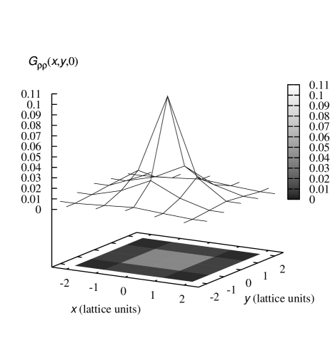
Figure 9: The nucleon density correlation $G_{\rho\rho}(\vec{n}_{s})$ for the triton in the $xy$-plane at imaginary time $t=0.143$ MeV^-1.

From $G_{\rho\rho}(\vec{n}_{s})$ we can also extract the root-mean-square radius for the total nucleon density.  In Fig. 10 we show the triton root-mean-square radius for the nucleon density as a function of imaginary time $t$.  We again fit to a decaying exponential form,

$$r_{\text{RMS}}(t)\rightarrow r_{\text{RMS}}+c^{\prime}e^{-\Delta E^{\prime}t},$$ (113)

and extract an asymptotic value of $2.27(7)$ fm.  This is about $30\%$ larger than the experimental value of $1.755(9)$ fm for the root-mean-square radius of the electric charge Amroun et al. (1994) and the point proton root-mean-square radius 1.60 fm Carlson and Schiavilla (1998). Similar values for the triton root-mean-square radius are also obtained in the pionless framework Platter and Hammer (2006).

Figure 10: The triton root-mean-square radius for total nucleon density versus imaginary time $t$.

XV Results for helium-4

For our simulations for helium-4 we use the same lattice parameters$\ a=(100$ MeV$)^{-1}$, $a_{t}=(70$ MeV$)^{-1}$, $C_{{}^{3}S_{1}}=-4.780\times 10^{-5}$ MeV^-2, $C_{{}^{1}S_{0}}=-3.414\times 10^{-5}$ MeV^-2, and $b=0.6$.  We again set $L=5$, $L_{t_{o}}=8$ and vary $L_{t_{i}}$ from $2$ to $10$. This time the standing waves comprising $\left|\Psi_{Z,N}^{\text{free}}\right\rangle$ are

$$\left\langle 0\right|a_{i,j}(\vec{n}_{s})\left|\psi_{1}\right\rangle =L^{-3/2}\delta_{i,0}\delta_{j,1},$$

$$\left\langle 0\right|a_{i,j}(\vec{n}_{s})\left|\psi_{2}\right\rangle =L^{-3/2}\delta_{i,0}\delta_{j,0},$$

$$\left\langle 0\right|a_{i,j}(\vec{n}_{s})\left|\psi_{3}\right\rangle =L^{-3/2}\delta_{i,1}\delta_{j,1},$$

$$\left\langle 0\right|a_{i,j}(\vec{n}_{s})\left|\psi_{4}\right\rangle =L^{-3/2}\delta_{i,1}\delta_{j,0}.$$ (114)

This corresponds with a helium-4 system with $J_{z}=0,J=0$ and total momentum zero.  For each value of $L_{t_{i}}$ we again produce about $5\times 10^{6}$ hybrid Monte Carlo trajectories using $2048$ processors running independent trajectories.

In Fig. 11 we show the energy for helium-4 as a function of imaginary time.

Figure 11: The transient energy for helium-4 as a function of imaginary time $t$.

If we fit $E(t)$ to a decaying exponential form at large $t$ we find an asymptotic value of $-21.5(9)$ MeV.  This is about $25\%$ smaller in magnitude than the experimental result of $-28.296$ MeV.  Note that we compare directly with the experimental value and have not corrected for small corrections due to electromagnetic effects.  In Fig. 12 we show the nucleon density correlation $G_{\rho\rho}(\vec{n}_{s})$ in the $xy$-plane at imaginary time $t=0.143$ MeV^-1.

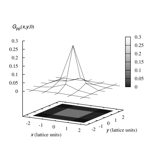
Figure 12: The nucleon density correlation $G_{\rho\rho}(\vec{n}_{s})$ for helium-4 in the $xy$-plane at imaginary time $t=0.143$ MeV^-1.

From $G_{\rho\rho}(\vec{n}_{s})$ we compute the root-mean-square radius for the total nucleon density, and in Fig. 13 we show the helium-4 root-mean-square radius for the total nucleon density as a function of imaginary time $t$.  Fitting to a decaying exponential form we find an asymptotic value of $r_{\text{RMS}}=1.50(14)$ fm.

Figure 13: The helium-4 root-mean-square radius for total nucleon density versus imaginary time $t$.

This is within $10\%$ of the experimentally observed value of $1.673(1)$ fm for the root-mean-square radius for the electric charge Borie and Rinker (1978) and the point proton root-mean-square radius 1.47 fm Carlson and Schiavilla (1998).

XVI Discussion

XVI.1 Room for more improvement

The lattice calculations in this study used leading-order chiral effective field theory with improved contact interactions of the form

$$f(\vec{q}_{s}\,^{2})\left[-\frac{1}{2}C\alpha_{t}\rho^{a^{{\dagger}},a}(\vec{q}_{s})\rho^{a^{{\dagger}},a}(-\vec{q}_{s})-\frac{1}{2}C_{I}\alpha_{t}\sum_{I=1,2,3}\rho_{I}^{a^{{\dagger}},a}(\vec{q}_{s})\rho_{I}^{a^{{\dagger}},a}(-\vec{q}_{s})\right],$$ (115)

where

$$f(\vec{q}_{s}\,^{2})=f_{0}^{-1}\exp\left[-b{\displaystyle\sum\limits_{l_{s}=1,2,3}}\left(1-\cos q_{l_{s}}\right)\right],$$ (116)

$$f_{0}=\frac{1}{L^{3}}\sum_{\vec{q}_{s}}\exp\left[-b{\displaystyle\sum\limits_{l_{s}=1,2,3}}\left(1-\cos q_{l_{s}}\right)\right].$$ (117)

The three unknown constants $C,C_{I},b$ were determined using the deuteron binding energy, ${}^{1}S_{0}$ scattering length, and the average effective range $\frac{1}{2}\left(r_{0}^{{}^{1}S_{0}}+r_{0}^{{}^{3}S_{1}}\right)$.  The scattering lengths and effective ranges were computed using Lüscher’s formula.  We used only one value for the lattice spacing, $a=(100$ MeV$)^{-1}$ and $a_{t}=(70$ MeV$)^{-1}$.  The simulations for triton and helium-4 were done at only one volume, a cubical lattice with length $L=5$ or $9.85$ fm.  In future studies both the dependence on the lattice spacings and finite volume should be investigated in some detail.

Lattice results for the deuteron root-mean-square radius and quadrupole moment agree with experimental values at the $5\%$ level.  The lattice calculation of the triton binding energy agrees with experiment to within $5\%,$ while the triton root-mean-square radius is larger by about $30\%$.  For helium-4 we find the binding energy is about $25\%$ smaller than experiment, while the root-mean-square radius agrees within $10\%$.  This is clear improvement over the first attempt with zero-range contact interactions which led to a clustering instability in the four-nucleon system. However, in order to make a more rigorous statement we also have to consider the full set of interactions which arise at next-to-leading order in chiral effective field theory.  We will discuss this procedure in future work.

XVI.2 Computational scaling

The lattice transfer matrix algorithm has several subroutines which scale differently with the number of nucleons $A$, the spatial volume $L^{3}$, and the total number of time steps $L_{t}=2L_{t_{o}}+L_{t_{i}}$.  Multiplication of the transfer matrices at each time step on the one-particle states scales as $A\times L^{3}\times L_{t}$.  Constructing the $A\times A$ matrix $\mathcal{M}(\pi_{I}^{\prime},s,s_{I},t^{\prime},t)$ from the inner products of the one-particle states scales as $A^{2}\times L^{3}$, while calculating the determinant of $\mathcal{M}(\pi_{I}^{\prime},s,s_{I},t^{\prime},t)$ scales as $A^{3}$ using $LU$ decomposition.  The molecular dynamics trajectories for the hybrid Monte Carlo updates involves computing the derivatives of $H_{HMC}$ with respect to $p_{\pi_{I}^{\prime}},p_{s},$ $p_{s_{I}},\pi_{I}^{\prime},s,s_{I}$.  The calculation of these derivatives require various loops which scale as $L^{3}\times L_{t}$, $L^{6}\times L_{t}$, and $A^{2}\times L^{3}\times L_{t}.$

With the same lattice parameters used in our triton and helium-4 simulations, we investigate the computational scaling for the transfer matrix algorithm as a function of the number of nucleons $A$.  We use $L=5$, $L_{t_{o}}=8$, $L_{t_{i}}=10$ and the free particle standing waves

$$\left\langle 0\right|a_{i,j}(\vec{n}_{s})\left|\psi_{1}\right\rangle =L^{-3/2}\delta_{i,0}\delta_{j,1},$$

$$\left\langle 0\right|a_{i,j}(\vec{n}_{s})\left|\psi_{2}\right\rangle =L^{-3/2}\delta_{i,0}\delta_{j,0},$$

$$\left\langle 0\right|a_{i,j}(\vec{n}_{s})\left|\psi_{3}\right\rangle =L^{-3/2}\delta_{i,1}\delta_{j,1},$$

$$\left\langle 0\right|a_{i,j}(\vec{n}_{s})\left|\psi_{4}\right\rangle =L^{-3/2}\delta_{i,1}\delta_{j,0},$$

$$\left\langle 0\right|a_{i,j}(\vec{n}_{s})\left|\psi_{5}\right\rangle =L^{-3/2}2^{1/2}\cos\left(\frac{2\pi n_{z}}{L}\right)\delta_{i,0}\delta_{j,1},$$

$$\left\langle 0\right|a_{i,j}(\vec{n}_{s})\left|\psi_{6}\right\rangle =L^{-3/2}2^{1/2}\cos\left(\frac{2\pi n_{z}}{L}\right)\delta_{i,0}\delta_{j,0},$$

$$\left\langle 0\right|a_{i,j}(\vec{n}_{s})\left|\psi_{7}\right\rangle =L^{-3/2}2^{1/2}\cos\left(\frac{2\pi n_{z}}{L}\right)\delta_{i,1}\delta_{j,1},$$

$$\left\langle 0\right|a_{i,j}(\vec{n}_{s})\left|\psi_{8}\right\rangle =L^{-3/2}2^{1/2}\cos\left(\frac{2\pi n_{z}}{L}\right)\delta_{i,1}\delta_{j,0}.$$ (118)

The initial state $\left|\Psi_{Z,N}^{\text{free}}\right\rangle$ is composed of all free particle standing waves $\left|\psi_{i}\right\rangle$ with $i\leq A$.  For $A=2$ this is the deuteron system, for $A=3$ the triton system, for $A=4$ helium-4, for $A=5$ helium-5, for $A=6$ lithium-6, for $A=7$ lithium-7, and for $A=8$ beryllium-8.  We note that for $A>4$ the momentum of $\left|\Psi_{Z,N}^{\text{free}}\right\rangle$ is not exactly zero but rather a wavepacket with a small spread in momentum centered around zero momentum.

In Fig. 14 we show the CPU times for $A=2,\cdots,8$ relative to the CPU time for $A=2$ with the same number of hybrid Monte Carlo trajectories.

Figure 14: CPU time versus the number of nucleons, $A$, measured relative to the $A=2$ deuteron system.

We see that for $A\leq 8$ the CPU time is approximately linear in $A$.  This suggests that the subroutines which scale as $A\times L^{3}\times L_{t}$ dominate the CPU time for the simulation for $A\leq 8$.

In Fig. 15 we show the average phase $\left\langle e^{i\theta}\right\rangle$ as defined in Eq. (101) versus the number of nucleons.  We note the relative maxima in $\left\langle e^{i\theta}\right\rangle$ at multiples of $4$.  This can be explained by the suppression of sign and phase oscillations due to approximate $SU(4)$ symmetry.  The $SU(4)$ suppression of oscillations is strongest for systems with equal numbers of spin-up and spin-down protons and neutrons. The results for the CPU time and average phase indicate that simulations of light nuclei with $A\leq 8$ can in fact be performed without much difficulty using the Monte Carlo transfer matrix algorithm presented here.  We plan to pursue these studies in future work.

Figure 15: The average phase $\left\langle e^{i\theta}\right\rangle$ versus the number of nucleons, $A$.

XVII Summary

We have described simulations of light nuclei on the lattice using a transfer matrix projection Monte Carlo method at leading order in chiral effective field theory.  We included lattice pion fields and auxiliary fields to reproduce the physics of instantaneous one-pion exchange and the leading-order S-wave contact interactions.  To avoid a clustering instability we also included higher-derivative contact interactions which adjust the S-wave scattering amplitude at higher momenta.  There are a total of three unknown constants, $C,C_{I},b,$ and these were determined using the deuteron binding energy, ${}^{1}S_{0}$ scattering length, and the average effective range $\frac{1}{2}\left(r_{0}^{{}^{1}S_{0}}+r_{0}^{{}^{3}S_{1}}\right)$.  We find agreement between lattice results and experimental data at the $5\%$ level for all calculated properties of the deuteron.  The lattice result for the triton binding energy agrees with experiment to within $5\%$ and the triton root-mean-square radius is within $30\%$.  For helium-4 the binding energy is within $25\%$ while the root-mean-square radius agrees within $10\%$.  We expect that the description will improve when higher-derivative operators are treated systematically by matching phase shifts on the lattice at higher momentum.  We have determined that the simulations for light nuclei with up to eight nucleons can be done without much difficulty using the lattice methods described here.

References

- Kuramashi et al. (1993) Y. Kuramashi, M. Fukugita, H. Mino, M. Okawa, and A. Ukawa, Phys. Rev. Lett. 71, 2387 (1993).
- Aoki et al. (2003) S. Aoki et al. (CP-PACS), Phys. Rev. D67, 014502 (2003), eprint hep-lat/0209124.
- Lin et al. (2003) C. J. D. Lin, G. Martinelli, E. Pallante, C. T. Sachrajda, and G. Villadoro, Phys. Lett. B553, 229 (2003), eprint hep-lat/0211043.
- Beane et al. (2006a) S. R. Beane, P. F. Bedaque, K. Orginos, and M. J. Savage (NPLQCD), Phys. Rev. D73, 054503 (2006a), eprint hep-lat/0506013.
- Fukugita et al. (1995) M. Fukugita, Y. Kuramashi, M. Okawa, H. Mino, and A. Ukawa, Phys. Rev. D52, 3003 (1995), eprint hep-lat/9501024.
- Beane et al. (2004) S. R. Beane, P. F. Bedaque, A. Parreno, and M. J. Savage, Phys. Lett. B585, 106 (2004), eprint hep-lat/0312004.
- Beane et al. (2006b) S. R. Beane, P. F. Bedaque, K. Orginos, and M. J. Savage, Phys. Rev. Lett. 97, 012001 (2006b), eprint hep-lat/0602010.
- Nogga et al. (2002) A. Nogga, H. Kamada, W. Glöckle, and B. R. Barrett, Phys. Rev. C65, 054003 (2002), eprint nucl-th/0112026.
- Machleidt et al. (1996) R. Machleidt, F. Sammarruca, and Y. Song, Phys. Rev. C53, 1483 (1996), eprint nucl-th/9510023.
- Machleidt (2001) R. Machleidt, Phys. Rev. C63, 024001 (2001), eprint nucl-th/0006014.
- Wiringa et al. (1995) R. B. Wiringa, V. G. J. Stoks, and R. Schiavilla, Phys. Rev. C51, 38 (1995), eprint nucl-th/9408016.
- Stoks et al. (1994) V. G. J. Stoks, R. A. M. Klomp, C. P. F. Terheggen, and J. J. de Swart, Phys. Rev. C49, 2950 (1994), eprint nucl-th/9406039.
- Coon and Glöckle (1981) S. A. Coon and W. Glöckle, Phys. Rev. C23, 1790 (1981).
- Coon and Han (2001) S. A. Coon and H. K. Han, Few Body Syst. 30, 131 (2001), eprint nucl-th/0101003.
- Pudliner et al. (1997) B. S. Pudliner, V. R. Pandharipande, J. Carlson, S. C. Pieper, and R. B. Wiringa, Phys. Rev. C56, 1720 (1997), eprint nucl-th/9705009.
- Glöckle et al. (1996) W. Glöckle, H. Witała, D. Hüber, H. Kamada, and J. Golak, Phys. Rept. 274, 107 (1996).
- Epelbaum et al. (2001) E. Epelbaum et al., Phys. Rev. Lett. 86, 4787 (2001), eprint nucl-th/0007057.
- Epelbaum et al. (2002a) E. Epelbaum et al., Phys. Rev. C66, 064001 (2002a), eprint nucl-th/0208023.
- Epelbaum et al. (1998a) E. Epelbaum, W. Glöckle, and U.-G. Meißner, Phys. Lett. B439, 1 (1998a), eprint nucl-th/9804005.
- Bogner et al. (2003a) S. K. Bogner, T. T. S. Kuo, A. Schwenk, D. R. Entem, and R. Machleidt, Phys. Lett. B576, 265 (2003a), eprint nucl-th/0108041.
- Bogner et al. (2003b) S. K. Bogner, T. T. S. Kuo, and A. Schwenk, Phys. Rept. 386, 1 (2003b), eprint nucl-th/0305035.
- Fujii et al. (2004) S. Fujii et al., Phys. Rev. C70, 024003 (2004), eprint nucl-th/0404049.
- Nogga et al. (2004) A. Nogga, S. K. Bogner, and A. Schwenk, Phys. Rev. C70, 061002 (2004), eprint nucl-th/0405016.
- Kievsky et al. (1993) A. Kievsky, S. Rosati, and M. Viviani, Nucl. Phys. A551, 241 (1993).
- Efros et al. (1994) V. D. Efros, W. Leidemann, and G. Orlandini, Phys. Lett. B338, 130 (1994), eprint nucl-th/9409004.
- Varga and Suzuki (1995) K. Varga and Y. Suzuki, Phys. Rev. C52, 2885 (1995), eprint nucl-th/9508023.
- Kievsky (1997) A. Kievsky, Nucl. Phys. A624, 125 (1997), eprint nucl-th/9706061.
- Wiringa et al. (2000) R. B. Wiringa, S. C. Pieper, J. Carlson, and V. R. Pandharipande, Phys. Rev. C62, 014001 (2000), eprint nucl-th/0002022.
- Pieper and Wiringa (2001) S. C. Pieper and R. B. Wiringa, Ann. Rev. Nucl. Part. Sci. 51, 53 (2001), eprint nucl-th/0103005.
- Pieper et al. (2001) S. C. Pieper, V. R. Pandharipande, R. B. Wiringa, and J. Carlson, Phys. Rev. C64, 014001 (2001), eprint nucl-th/0102004.
- Pieper et al. (2002) S. C. Pieper, K. Varga, and R. B. Wiringa, Phys. Rev. C66, 044310 (2002), eprint nucl-th/0206061.
- Wiringa and Pieper (2002) R. B. Wiringa and S. C. Pieper, Phys. Rev. Lett. 89, 182501 (2002), eprint nucl-th/0207050.
- Pieper et al. (2004) S. C. Pieper, R. B. Wiringa, and J. Carlson, Phys. Rev. C70, 054325 (2004), eprint nucl-th/0409012.
- Fantoni et al. (2001) S. Fantoni, A. Sarsa, and K. E. Schmidt, Phys. Rev. Lett. 87, 181101 (2001), eprint nucl-th/0106026.
- Sarsa et al. (2003) A. Sarsa, S. Fantoni, K. E. Schmidt, and F. Pederiva, Phys. Rev. C68, 024308 (2003), eprint nucl-th/0303035.
- Pederiva et al. (2004) F. Pederiva, A. Sarsa, K. E. Schmidt, and S. Fantoni, Nucl. Phys. A742, 255 (2004), eprint nucl-th/0403069.
- Chang et al. (2004) S. Y. Chang et al., Nucl. Phys. A746, 215 (2004), eprint nucl-th/0401016.
- Navratil et al. (2000) P. Navratil, J. P. Vary, and B. R. Barrett, Phys. Rev. Lett. 84, 5728 (2000), eprint nucl-th/0004058.
- Fayache et al. (2001) M. S. Fayache, J. P. Vary, B. R. Barrett, P. Navratil, and S. Aroua (2001), eprint nucl-th/0112066.
- Navratil and Ormand (2003) P. Navratil and W. E. Ormand, Phys. Rev. C68, 034305 (2003), eprint nucl-th/0305090.
- Caurier and Navratil (2006) E. Caurier and P. Navratil, Phys. Rev. C73, 021302 (2006), eprint nucl-th/0512015.
- Forssen et al. (2005) C. Forssen, P. Navratil, W. E. Ormand, and E. Caurier, Phys. Rev. C71, 044312 (2005), eprint nucl-th/0412049.
- Nogga et al. (2006) A. Nogga, P. Navratil, B. R. Barrett, and J. P. Vary, Phys. Rev. C73, 064002 (2006), eprint nucl-th/0511082.
- Stetcu et al. (2006) I. Stetcu, B. R. Barrett, and U. van Kolck (2006), eprint nucl-th/0609023.
- Kamada et al. (2001) H. Kamada et al., Phys. Rev. C64, 044001 (2001), eprint nucl-th/0104057.
- Carlson and Schiavilla (1998) J. Carlson and R. Schiavilla, Rev. Mod. Phys. 70, 743 (1998).
- Müller et al. (2000) H. M. Müller, S. E. Koonin, R. Seki, and U. van Kolck, Phys. Rev. C61, 044320 (2000), eprint nucl-th/9910038.
- Lee et al. (2004) D. Lee, B. Borasoy, and T. Schäfer, Phys. Rev. C70, 014007 (2004), eprint nucl-th/0402072.
- Hubbard (1959) J. Hubbard, Phys. Rev. Lett. 3, 77 (1959).
- Stratonovich (1958) R. L. Stratonovich, Soviet Phys. Doklady 2, 416 (1958).
- Duane et al. (1987) S. Duane, A. D. Kennedy, B. J. Pendleton, and D. Roweth, Phys. Lett. B195, 216 (1987).
- Borasoy et al. (2006) B. Borasoy, H. Krebs, D. Lee, and U.-G. Meißner, Nucl. Phys. A768, 179 (2006), eprint nucl-th/0510047.
- Jenkins and Manohar (1991) E. Jenkins and A. V. Manohar, Phys. Lett. B255, 558 (1991).
- Bernard et al. (1992) V. Bernard, N. Kaiser, J. Kambor, and U. G. Meißner, Nucl. Phys. B388, 315 (1992).
- Becher and Leutwyler (1999) T. Becher and H. Leutwyler, Eur. Phys. J. C9, 643 (1999), eprint hep-ph/9901384.
- Weinberg (1990) S. Weinberg, Phys. Lett. B251, 288 (1990).
- Weinberg (1991) S. Weinberg, Nucl. Phys. B363, 3 (1991).
- Epelbaum (2000) E. Epelbaum, Dissertation Jülich (2000).
- Lee (2004) D. Lee, Phys. Rev. C70, 064002 (2004), eprint nucl-th/0407088.
- Epelbaum et al. (1998b) E. Epelbaum, W. Glöckle, and U.-G. Meißner, Nucl. Phys. A637, 107 (1998b), eprint nucl-th/9801064.
- Krebs et al. (2005) H. Krebs, V. Bernard, and U.-G. Meißner, Ann. Phys. 316, 160 (2005), eprint nucl-th/0407078.
- Ordonez et al. (1996) C. Ordonez, L. Ray, and U. van Kolck, Phys. Rev. C53, 2086 (1996), eprint hep-ph/9511380.
- Kaiser et al. (1997) N. Kaiser, R. Brockmann, and W. Weise, Nucl. Phys. A625, 758 (1997), eprint nucl-th/9706045.
- Creutz (1988) M. Creutz, Phys. Rev. D38, 1228 (1988).
- Creutz (2000) M. Creutz, Found. Phys. 30, 487 (2000), eprint hep-lat/9905024.
- Lanczos (1950) C. Lanczos, J. Res. Nat. Bur. Stand. 45, 255 (1950).
- Lüscher (1986) M. Lüscher, Commun. Math. Phys. 105, 153 (1986).
- Seki and van Kolck (2006) R. Seki and U. van Kolck, Phys. Rev. C73, 044006 (2006), eprint nucl-th/0509094.
- Epelbaum et al. (2002b) E. Epelbaum, U. G. Meißner, W. Glöckle, and C. Elster, Phys. Rev. C65, 044001 (2002b), eprint nucl-th/0106007.
- Lee (2006a) D. Lee, Phys. Rev. A73, 063204 (2006a), eprint physics/0512085.
- Wu et al. (2003) C. Wu, J. Hu, and S.-C. Zhang, Phys. Rev. Lett. 91, 186402 (2003), eprint cond-mat/0302165.
- Wu (2005) C. Wu, Phys. Rev. Lett. 95, 266404 (2005), eprint cond-mat/0409247.
- Lee and Schäfer (2006) D. Lee and T. Schäfer, Phys. Rev. C73, 015202 (2006), eprint nucl-th/0509018.
- Thomas (1935) L. H. Thomas, Phys. Rev. 47, 903 (1935).
- Efimov (1971) V. N. Efimov, Sov. J. Nucl. Phys. 12, 589 (1971).
- Efimov (1993) V. N. Efimov, Phys. Rev. C47, 1876 (1993).
- Bedaque et al. (1999a) P. F. Bedaque, H.-W. Hammer, and U. van Kolck, Phys. Rev. Lett. 82, 463 (1999a), eprint nucl-th/9809025.
- Bedaque et al. (1999b) P. F. Bedaque, H.-W. Hammer, and U. van Kolck, Nucl. Phys. A646, 444 (1999b), eprint nucl-th/9811046.
- Bedaque et al. (2000) P. F. Bedaque, H.-W. Hammer, and U. van Kolck, Nucl. Phys. A676, 357 (2000), eprint nucl-th/9906032.
- Braaten and Hammer (2006) E. Braaten and H.-W. Hammer, Phys. Rept. 428, 259 (2006).
- Platter (2006) L. Platter, Phys. Rev. C74, 037001 (2006), eprint nucl-th/0606006.
- Platter et al. (2004) L. Platter, H.-W. Hammer, and U.-G. Meißner, Phys. Rev. A70, 052101 (2004), eprint cond-mat/0404313.
- Platter et al. (2005) L. Platter, H.-W. Hammer, and U.-G. Meißner, Phys. Lett. B607, 254 (2005), eprint nucl-th/0409040.
- Lee (2006b) D. Lee, Phys. Rev. B73, 115112 (2006b), eprint cond-mat/0511332.
- Lee (2005) D. Lee, Phys. Rev. C71, 044001 (2005), eprint nucl-th/0407101.
- Chen et al. (2004) J.-W. Chen, D. Lee, and T. Schäfer, Phys. Rev. Lett. 93, 242302 (2004), eprint nucl-th/0408043.
- (87) D. Lee, eprint cond-mat/0606706.
- Amroun et al. (1994) A. Amroun et al., Nucl. Phys. A579, 596 (1994).
- Platter and Hammer (2006) L. Platter and H. W. Hammer, Nucl. Phys. A766, 132 (2006), eprint nucl-th/0509045.
- Borie and Rinker (1978) E. Borie and G. A. Rinker, Phys. Rev. A18, 324 (1978).