Axial, induced pseudoscalar, and pion-nucleon form factors in manifestly Lorentz-invariant chiral perturbation theory

Abstract

We calculate the nucleon form factors $G_{A}$ and $G_{P}$ of the isovector axial-vector current and the pion-nucleon form factor $G_{\pi N}$ in manifestly Lorentz-invariant baryon chiral perturbation theory up to and including order ${\cal O}(p^{4})$. In addition to the standard treatment including the nucleon and pions, we also consider the axial-vector meson $a_{1}$ as an explicit degree of freedom. This is achieved by using the reformulated infrared renormalization scheme. We find that the inclusion of the axial-vector meson effectively results in one additional low-energy coupling constant that we determine by a fit to the data for $G_{A}$. The inclusion of the axial-vector meson results in an improved description of the experimental data for $G_{A}$, while the contribution to $G_{P}$ is small.

I Introduction

The electroweak form factors are sets of functions that are used to parameterize the structure of the nucleon as seen by the electromagnetic and the weak probes. While a wealth of data and theoretical predictions exist for the electromagnetic form factors (see, e.g., Gao:2003ag ; Friedrich:2003iz ; Hyde-Wright:2004gh and references therein), the nucleon form factors of the isovector axial-vector current, the axial form factor $G_{A}(q^{2})$ and, in particular, the induced pseudoscalar form factor $G_{P}(q^{2})$, are not as well-known (see, e.g., Bernard:2001rs ; Gorringe:2002xx for a review). However, there are ongoing efforts to increase our understanding of these form factors. The value of the axial form factor at zero momentum transfer is defined as the axial-vector coupling constant $g_{A}$ and is quite precisely determined from neutron beta decay. The $q^{2}$ dependence of the axial form factor can be obtained either through neutrino scattering or pion electroproduction (see Bernard:2001rs and references therein). The second method makes use of the so-called Adler-Gilman relation Adler:1966 which provides a chiral Ward identity establishing a connection between charged pion electroproduction at threshold and the isovector axial-vector current evaluated between single-nucleon states (see, e.g., Scherer:1991cy for more details). The induced pseudoscalar form factor $G_{P}(q^{2})$ is even less known than $G_{A}(q^{2})$. It has been investigated in ordinary and radiative muon capture as well as pion electroproduction. Analogous to the axial-vector coupling constant $g_{A}$, the induced pseudoscalar coupling constant is defined through $g_{P}=\frac{m_{\mu}}{2m_{N}}G_{P}(q^{2}=-0.88m_{\mu}^{2})$, where $q^{2}=-0.88\,m_{\mu}^{2}$ corresponds to muon capture kinematics and the additional factor $\frac{m_{\mu}}{2m_{N}}$ stems from a different convention used in muon capture. For a comprehensive review on the experimental and theoretical situation concerning $G_{P}(q^{2})$ see for example Gorringe:2002xx . A discrepancy between the results in ordinary and radiative muon capture has recently been addressed in Clark:2005as . Theoretical approaches to the axial and induced pseudoscalar form factors include the early current algebra and PCAC calculations Adler:1966 ; Nambu:1997wb ; Sato:1967 , various quark model (see, e.g., Tegen:1983gg ; Hwang:1984sz ; Boffi:2001zb ; Merten:2002nz ; Ma:2002xu ; Khosonthongkee:2004qm ; Silva:2005fa ) and lattice calculations Liu:1992ab . For a recent discussion on extracting the axial form factor in the timelike region from $\bar{p}+n\to\pi^{-}+\ell^{-}+\ell^{+}$ ($\ell=e$ or $\mu$) see Adamuscin:2006bk . Chiral perturbation theory (ChPT) Weinberg:1978kz ; Gasser:1984yg ; Gasser:1984gg ; Gasser:1988rb is the low-energy effective theory of the standard model and as such allows model-independent calculations of nucleon properties (see Bernard:1995dp ; Scherer:2002tk for an introduction). The axial form factor has been addressed in the framework of heavy-baryon ChPT Bernard:1992ys ; Bernard:1993bq ; Fearing:1997dp ; Bernard:1998gv . In principle, when considering a charged transition there is a third form factor, the induced pseudotensorial form factor $G_{T}(q^{2})$. As will be explained below, this form factor vanishes when combining isospin symmetry and charge-conjugation invariance and therefore is not considered in this work Weinberg:1958ut . Experimentally the induced pseudotensorial form factor is found to be small Wilkinson:2000gx ; Minamisono:2001cd . Finally, defining the pion-nucleon form factor in terms of the pseudoscalar quark density and using the partially conserved axial-vector current (PCAC) relation allows one to determine the pion-nucleon form factor, once the axial and induced pseudoscalar form factors are known.

In this paper we calculate the axial, the induced pseudoscalar, and the pion nucleon form factors of the nucleon in manifestly Lorentz-invariant ChPT up to and including order ${\cal O}(p^{4})$. The renormalization procedure is performed in the framework of the infrared renormalization of Becher:1999he . In its reformulated version Schindler:2003xv , this renormalization scheme allows for the inclusion of further degrees of freedom. In the following we will include the $a_{1}$ axial-vector meson as an explicit degree of freedom. It needs to be pointed out that in a strict chiral expansion up to order ${\cal O}(p^{4})$ the results will not differ from the ones obtained in the standard framework. However, explicitly keeping all terms generated from the considered diagrams involving the axial-vector meson amounts to a resummation of higher-order contributions. This phenomenological approach has shown an improved description of the electromagnetic form factors of the nucleon Kubis:2000zd ; Schindler:2005ke when the $\rho$, $\omega$, and $\phi$ mesons are included.

This paper is organized as follows: In Sec. II the definitions and some important properties of the relevant form factors are given. Section III contains the effective Lagrangians used in the present calculation. We present and discuss the results for the form factors with and without the inclusion of the axial-vector meson $a_{1}$ in Sec. IV. Section V contains a short summary.

II Definition and properties of the isovector axial-vector current

In QCD, the three components of the isovector axial-vector current are defined as

$$A^{\mu,a}(x)\equiv\bar{q}(x)\gamma^{\mu}\gamma_{5}\frac{\tau^{a}}{2}q(x),\quad q=\left(\begin{array}[]{c}u\\ d\end{array}\right),\quad a=1,2,3.$$ (1)

The operators $A^{\mu,a}(x)$ satisfy the following properties relevant for the subsequent discussion:

1. Hermiticity:

   $$A^{\mu,a\dagger}(x)=A^{\mu,a}(x).$$ (2)

2. Equal-time commutation relations with the vector charges:

   $$[Q^{a}_{V}(t),A^{\mu,b}(t,\vec{x})]=i\epsilon^{abc}A^{\mu,c}(t,\vec{x}).$$ (3)

3. Transformation behavior under parity:

   $$A^{\mu,a}(x)\stackrel{{\scriptstyle\cal P}}{{\mapsto}}-A_{\mu}^{a}(\tilde{x}),\quad\tilde{x}^{\mu}=x_{\mu}.$$ (4)

4. Transformation behavior under charge conjugation:

   $$A^{\mu,a}(x) \stackrel{{\scriptstyle{\cal C}}}{{\mapsto}} A^{\mu,a}(x),\quad a=1,3,$$

   $$A^{\mu,2}(x) \stackrel{{\scriptstyle{\cal C}}}{{\mapsto}} -A^{\mu,2}(x).$$ (5)

5. Partially conserved axial-vector current (PCAC) relation:

   $$\partial_{\mu}A^{\mu,a}=i\bar{q}\gamma_{5}\{\frac{\tau^{a}}{2},{\cal M}\}q,$$ (6)

   where ${\cal M}=\mbox{diag}(m_{u},m_{d})$ is the quark mass matrix.

Assuming isospin symmetry, $m_{\mu}=m_{d}=\hat{m}$, the most general parametrization of the isovector axial-vector current evaluated between one-nucleon states in terms of axial-vector covariants is given by

$$\langle N(p^{\prime})|A^{\mu,a}(0)|N(p)\rangle=\bar{u}(p^{\prime})\left[\gamma^{\mu}\gamma_{5}G_{A}(q^{2})+\frac{q^{\mu}}{2m_{N}}\gamma_{5}G_{P}(q^{2})\right]\frac{\tau^{a}}{2}u(p),$$ (7)

where $q_{\mu}=p^{\prime}_{\mu}-p_{\mu}$ and $m_{N}$ denotes the nucleon mass. $G_{A}(q^{2})$ is called the axial form factor and $G_{P}(q^{2})$ is the induced pseudoscalar form factor. From the Hermiticity of Eq. (2), we find that $G_{A}$ and $G_{P}$ are real for space-like momenta ($q^{2}\leq 0$). In the case of perfect isospin symmetry the strong interactions are invariant under ${\cal G}$ conjugation, which is a combination of charge conjugation $\cal C$ and a rotation by $\pi$ about the 2 axis in isospin space (charge symmetry operation),

$${\cal G}={\cal C}\exp(i\pi Q_{V}^{2}).$$ (8)

The presence of a third so-called second-class structure Weinberg:1958ut of the type $i\sigma^{\mu\nu}q_{\nu}\gamma_{5}$ in the charged transition would indicate a violation of $\cal G$ conjugation. As there seems to be no clear empirical evidence for such a contribution Wilkinson:2000gx ; Minamisono:2001cd we will omit it henceforth.

Similarly, the nucleon matrix element of the pseudoscalar density $P^{a}(x)=i\bar{q}(x)\gamma_{5}\tau^{a}q(x)$ can be parameterized as

$$\hat{m}\langle N(p^{\prime})|P^{a}(0)|N(p)\rangle=\frac{M_{\pi}^{2}F_{\pi}}{M_{\pi}^{2}-q^{2}}G_{\pi N}(q^{2})i\bar{u}(p^{\prime})\gamma_{5}\tau^{a}u(p),$$ (9)

where $M_{\pi}$ is the pion mass and $F_{\pi}$ the pion decay constant. Equation (9) defines the form factor $G_{\pi N}(q^{2})$ in terms of the QCD operator $\hat{m}P^{a}(x)$. The operator $\hat{m}P^{a}(x)/(M_{\pi}^{2}F_{\pi})$ serves as an interpolating pion field and thus $G_{\pi N}(q^{2})$ is also referred to as the pion-nucleon form factor for this specific choice of the interpolating pion field Bernard:1995dp . The pion-nucleon coupling constant $g_{\pi N}$ is defined through $G_{\pi N}(q^{2})$ evaluated at $q^{2}=M_{\pi}^{2}$. As a result of the PCAC relation, Eq. (6), the three form factors $G_{A}$, $G_{P}$, and $G_{\pi N}$ are related by

$$2m_{N}G_{A}(q^{2})+\frac{q^{2}}{2m_{N}}G_{P}(q^{2})=2\frac{M_{\pi}^{2}F_{\pi}}{M_{\pi}^{2}-q^{2}}G_{\pi N}(q^{2}).$$ (10)

III Effective Lagrangian and power counting

The calculation of the isovector axial-vector current form factors of the nucleon requires both the purely mesonic as well as the one-nucleon part of the chiral effective Lagrangian up to order ${\cal O}(p^{4})$,

$${\cal L}_{\rm eff}={\cal L}_{2}+{\cal L}_{4}+{\cal L}^{(1)}_{{\pi}N}+{\cal L}^{(2)}_{{\pi}N}+{\cal L}^{(3)}_{{\pi}N}+{\cal L}^{(4)}_{{\pi}N}+\cdots.$$ (11)

Here, $p$ collectively stands for a “small” quantity such as the pion mass, a small external four-momentum of the pion or of an external source, and an external three-momentum of the nucleon.

The pion fields are contained in the $2\times 2$ matrix $U$,

$$U(x) = u^{2}(x)=\exp\left(\frac{i\Phi(x)}{F}\right),$$ (12)

$$\Phi = \vec{\tau}\cdot\vec{\phi}=\left(\begin{array}[]{cc}\pi^{0}&\sqrt{2}\pi^{+}\\ \sqrt{2}\pi^{-}&-\pi^{0}\end{array}\right),$$ (15)

and the purely mesonic Lagrangian at order ${\cal O}(p^{2})$ is given by Gasser:1984yg

$${\cal L}_{2}=\frac{F^{2}}{4}\mbox{Tr}\left[D_{\mu}U(D^{\mu}U)^{\dagger}\right]+\frac{F^{2}}{4}\mbox{Tr}\left[\chi U^{\dagger}+U\chi^{\dagger}\right].$$ (16)

The covariant derivative $D_{\mu}U$ with a coupling to an external axial-vector field $a_{\mu}=\tau^{a}a^{a}_{\mu}/2$ only is given by

$$D_{\mu}U=\partial_{\mu}U-ia_{\mu}U-iUa_{\mu}\,,$$

while $\chi$ is defined as

$$\chi=2B(s+ip),$$

with $s$ and $p$ the scalar and pseudoscalar external sources, respectively. $F$ denotes the pion decay constant in the chiral limit, $F_{\pi}=F[1+{\cal O}(\hat{m})]=92.42(26)$ MeV Yao:2006 . We work in the isospin-symmetric limit $m_{u}=m_{d}=\hat{m}$, and the lowest-order expression for the squared pion mass is $M^{2}=2B\hat{m}$, where $B$ is related to the quark condensate $\langle\bar{q}q\rangle_{0}$ in the chiral limit Gasser:1984yg ; Colangelo:2001sp , $\langle\bar{u}u\rangle_{0}=\langle\bar{d}d\rangle_{0}=-F^{2}B$.

For the mesonic Lagrangian at order ${\cal O}(p^{4})$ we only list the term that contributes to our calculation,

$${\cal L}_{4}=\cdots+\frac{l_{4}}{8}\mbox{Tr}\left[D_{\mu}U(D^{\mu}U)^{\dagger}\right]\mbox{Tr}\left[\chi U^{\dagger}+U\chi^{\dagger}\right]+\cdots\,.$$ (17)

The complete list for the $SU(2)$ case can be found in Gasser:1988rb .

The lowest-order pion-nucleon Lagrangian is given by Gasser:1988rb

$${\cal L}^{(1)}_{\pi N}=\bar{\Psi}\left(iD/\hskip 1.00006pt-m+\frac{\texttt{g}_{A}}{2}\,\gamma^{\mu}\gamma_{5}u_{\mu}\right)\Psi,$$ (18)

with $m$ the nucleon mass and $\texttt{g}_{A}$ the axial-vector coupling constant both evaluated in the chiral limit.

For the nucleonic Lagrangians of higher orders we only display those terms that contribute to our calculations. A complete list of terms at orders ${\cal O}(p^{2})$ and ${\cal O}(p^{3})$ can be found in Gasser:1988rb ; Fettes:2000gb . At second order the Lagrangian reads

$${\cal L}_{{\pi}N}^{(2)} = c_{1}\mbox{Tr}(\chi_{+})\bar{\Psi}\Psi-\frac{c_{2}}{4m^{2}}\left[\bar{\Psi}\mbox{Tr}\left(u_{\mu}u_{\nu}\right)D^{\mu}D^{\nu}\Psi+\mbox{h.c.}\right]+\frac{c_{3}}{2}\,\bar{\Psi}\mbox{Tr}\left(u_{\mu}u^{\mu}\right)\Psi$$ (19)

$$-\frac{c_{4}}{4}\bar{\Psi}\gamma^{\mu}\gamma^{\nu}[u_{\mu},u_{\nu}]\Psi+\cdots,$$

while at order ${\cal O}(p^{3})$ we need

$${\cal L}_{{\pi}N}^{(3)}=\frac{d_{16}}{2}\bar{\Psi}\gamma^{\mu}\gamma_{5}\mbox{Tr}(\chi_{+})u_{\mu}\Psi+\frac{d_{22}}{2}\bar{\Psi}\gamma^{\mu}\gamma_{5}\left[D_{\nu},F_{\mu\nu}^{-}\right]\Psi+\cdots\,.$$ (20)

There are no contributions from ${\cal L}^{(4)}_{{\pi}N}$ in our calculation. The Lagrangians contain the building blocks

$$D_{\mu}\Psi = \left(\partial_{\mu}+\Gamma_{\mu}\right)\Psi,$$

$$\Gamma_{\mu} = \frac{1}{2}\,\left[u^{\dagger}\left(\partial_{\mu}-ia_{\mu}\right)u+u\left(\partial_{\mu}-ia_{\mu}\right)u^{\dagger}\right],$$

$$u_{\mu} = i\left[u^{\dagger}\partial_{\mu}u-u\partial_{\mu}u^{\dagger}-i(u^{\dagger}a_{\mu}u+ua_{\mu}u^{\dagger})\right],$$

$$\chi_{+} = u^{\dagger}\chi u^{\dagger}+u\chi^{\dagger}u,$$

$$F^{-}_{\mu\nu} = u^{\dagger}(\partial_{\mu}a_{\nu}-\partial_{\nu}a_{\mu}-i[a_{\mu},a_{\nu}])u+u(\partial_{\mu}a_{\nu}-\partial_{\nu}a_{\mu}+i[a_{\mu},a_{\nu}])u^{\dagger},$$

where we only display the external axial-vector source $a_{\mu}$.

In order to include axial-vector mesons as explicit degrees of freedom we consider the vector-field formulation of Ecker:yg in which the $a_{1}(1260)$ meson is represented by $A_{\mu}=A_{\mu}^{a}\tau^{a}$. The advantage of this formulation is that the coupling of the axial-vector mesons to pions and external sources is at least of order ${\cal O}(p^{3})$. A complete list of possible couplings at this order can be found in Ecker:yg . The calculation of the contributions to the isovector axial-vector form factors only requires the term

$${\cal L}_{{\pi}A}^{(3)}=\frac{f_{A}}{4}\mbox{Tr}(A_{\mu\nu}F^{\mu\nu}_{-}),$$ (21)

where

$$A_{\mu\nu}=\nabla_{\mu}A_{\nu}-\nabla_{\nu}A_{\mu}$$

with

$$\nabla_{\mu}A_{\nu}=\partial_{\mu}A_{\nu}+[\Gamma_{\mu},A_{\nu}].$$

The coupling of the axial-vector meson to the nucleon starts at order ${\cal O}(p^{0})$. The corresponding Lagrangian reads

$${\cal L}_{NA}^{(0)}=\frac{g_{a_{1}}}{2}\bar{\Psi}\gamma^{\mu}\gamma_{5}A_{\mu}\Psi.$$ (22)

A calculation up to order ${\cal O}(p^{4})$ would in principle also require the Lagrangian of order ${\cal O}(p)$. However, there is no term at this order that is allowed by the symmetries.

In addition to the usual counting rules for pions and nucleons (see, e.g., Scherer:2002tk ), we count the axial-vector meson propagator as order ${\cal O}(p^{0})$, vertices from ${\cal L}_{{\pi}A}^{(3)}$ as order ${\cal O}(p^{3})$ and vertices from ${\cal L}_{AN}^{(0)}$ as order ${\cal O}(p^{0})$, respectively Fuchs:2003sh .

IV Results and Discussion

IV.1 Results without axial-vector mesons

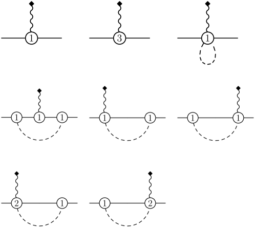
Figure 1: One-particle-irreducible diagrams contributing to the nucleon matrix element of the isovector axial-vector current.

The axial form factor $G_{A}(q^{2})$ only receives contributions from the one-particle-irreducible diagrams of Fig. 1. The unrenormalized result reads

$${G_{A}}_{0}(q^{2}) = \texttt{g}_{A}+4M^{2}d_{16}-d_{22}q^{2}-\frac{\texttt{g}_{A}}{F^{2}}I_{\pi}+2\frac{\texttt{g}_{A}}{F^{2}}M^{2}I_{{\pi}N}(m_{N}^{2})$$ (23)

$$+8\frac{\texttt{g}_{A}}{F^{2}}m_{N}\left\{c_{4}\left[M^{2}I_{{\pi}N}(m_{N}^{2})-I_{{\pi}N}^{(00)}(m_{N}^{2})\right]-c_{3}I_{{\pi}N}^{(00)}(m_{N}^{2})\right\}$$

$$-\frac{\texttt{g}_{A}^{3}}{4F^{2}}\left[I_{\pi}-4m_{N}^{2}I_{{\pi}N}^{(p)}(m_{N}^{2})+4m_{N}^{2}(n-2)I_{{\pi}NN}^{(00)}(q^{2})\right.$$

$$\left.+16m_{N}^{4}I_{{\pi}NN}^{(PP)}(q^{2})+4m_{N}^{2}tI_{{\pi}NN}^{(qq)}(q^{2})\right].$$

The definition of the integrals can be found in the appendix. To renormalize the expression for $G_{A}(q^{2})$ we multiply Eq. (23) by the nucleon wave function renormalization constant $Z$ Becher:1999he ,

$$Z=1-\frac{9\texttt{g}_{A}^{2}M^{2}}{32\pi^{2}F^{2}}\left[\frac{1}{3}+\ln\left(\frac{M}{m}\right)\right]+\frac{9\texttt{g}_{A}^{2}M^{3}}{64\pi F^{2}m},$$ (24)

and replace the integrals with their infrared singular parts.

The axial-vector coupling constant $g_{A}$ is defined as $g_{A}=G_{A}(q^{2}=0)=1.2695(29)$ Yao:2006 and we obtain for its quark-mass expansion

$$g_{A}=\texttt{g}_{A}+g_{A}^{(1)}M^{2}+g_{A}^{(2)}M^{2}\ln\left(\frac{M}{m}\right)+g_{A}^{(3)}M^{3}+{\cal O}(M^{4}),$$ (25)

with

$$g_{A}^{(1)} = 4d_{16}-\frac{\texttt{g}_{A}^{3}}{16\pi^{2}F^{2}}\,,$$

$$g_{A}^{(2)} = -\frac{\texttt{g}_{A}}{8\pi^{2}F^{2}}(1+2\texttt{g}_{A}^{2})\,,$$

$$g_{A}^{(3)} = \frac{\texttt{g}_{A}}{8\pi F^{2}m}(1+\texttt{g}_{A}^{2})-\frac{\texttt{g}_{A}}{6\pi F^{2}}(c_{3}-2c_{4}),$$ (26)

where all coefficients are understood as IR renormalized parameters. These results agree with the chiral coefficients obtained in HBChPT Kambor:1998pi ; Bernard:2006te as well as the IR calculation of Ando:2006xy . It is worth noting that an agreement for the analytic term $g_{A}^{(1)}$ cannot be expected in general. For example, when expressed in terms of the renormalized couplings of the extended on-mass-shell (EOMS) renormalization scheme of Fuchs:2003qc , the $g_{A}^{(1)}$ coefficient is given by Ando:2006xy

$$4d_{16}^{EOMS}-\frac{\texttt{g}_{A}}{16\pi^{2}F^{2}}(2+3\texttt{g}_{A}^{2})+\frac{c_{1}\texttt{g}_{A}m}{4\pi^{2}F^{2}}(4-\texttt{g}_{A}^{2}).$$

Such a difference is not a surprise, because the use of different renormalization schemes is compensated by different values of the renormalized parameters. For a similar discussion regarding the chiral expansion of the nucleon mass, see Fuchs:2003qc .

The axial form factor can be written as

$$G_{A}(q^{2})=g_{A}+\frac{1}{6}\,g_{A}\,\langle r^{2}_{A}\rangle\,q^{2}+\frac{\texttt{g}_{A}^{3}}{4F^{2}}H(q^{2}),$$ (27)

where $\langle r^{2}_{A}\rangle$ is the axial mean-square radius and $H(q^{2})$ contains loop contributions and satisfies $H(0)=H^{\prime}(0)=0$. The low-energy coupling constants (LECs) $d_{16}$ and $d_{22}$ are thus absorbed in the axial-vector coupling constant $g_{A}$ and the axial mean-square radius $\langle r^{2}_{A}\rangle$. The numerical contribution of $H(q^{2})$ is negligible which can be understood by expanding $H$ in a Taylor series in $q^{2}$. Such an expansion generates powers of $q^{2}/m^{2}$ where the individual coefficients have a chiral expansion similar to Eq. (25).

For the analysis of experimental data, $G_{A}(q^{2})$ is conventionally parameterized using a dipole form as

$$G_{A}(q^{2})=\frac{g_{A}}{(1-\frac{q^{2}}{M^{2}_{A}})^{2}},$$ (28)

where the so-called axial mass $M_{A}$ is related to the axial root-mean-square radius by $\langle r^{2}_{A}\rangle^{\frac{1}{2}}=2\sqrt{3}/M_{A}$. The global average for the axial mass extracted from neutrino scattering experiments given in Liesenfeld:1999mv is

$$M_{A}=(1.026\pm 0.021)\,\mbox{GeV},$$ (29)

whereas a recent analysis Budd:2003wb taking account of updated expressions for the vector form factors finds a slightly smaller value

$$M_{A}=(1.001\pm 0.020)\,\mbox{GeV}.$$ (30)

On the other hand, smaller values of $(0.95\pm 0.03)$ GeV and $(0.96\pm 0.03)$ GeV have been obtained in Kuzmin:2006dh as world averages from quasielastic scattering and $(1.12\pm 0.03)$ GeV from single pion neutrinoproduction. Finally, the most recent result extracted from quasielastic $\nu_{\mu}n\to\mu^{-}p$ in oxygen nuclei reported by the K2K Collaboration, $M_{A}=(1.20\pm 0.12)$ GeV, is considerably larger Gran:2006jn .

The extraction of the axial mean-square radius from charged pion electroproduction at threshold is motivated by the current algebra results and the PCAC hypothesis. The most recent result for the reaction $p(e,e^{\prime}\pi^{+})n$ has been obtained at MAMI at an invariant mass of $W=1125$ MeV (corresponding to a pion center-of-mass momentum of $|\vec{q}^{\ast}|=112$ MeV) and photon four-momentum transfers of $-k^{2}=0.117$, $0.195$ and 0.273 GeV² Liesenfeld:1999mv . Using an effective-Lagrangian model an axial mass of

$$\bar{M}_{A}=(1.077\pm 0.039)\,\mbox{GeV}$$

was extracted, where the bar is used to distinguish the result from the neutrino scattering value. In the meantime, the experiment has been repeated including an additional value of $-k^{2}=0.058$ GeV² Baumann:2004 and is currently being analyzed. The global average from several pion electroproduction experiments is given by Bernard:2001rs

$$\bar{M}_{A}=(1.068\pm 0.017)\,\mbox{GeV}.$$ (31)

It can be seen that the values of Eqs. (29) and (30) for the neutrino scattering experiments are smaller than that of Eq. (31) for the pion electroproduction experiments. The discrepancy was explained in heavy baryon chiral perturbation theory Bernard:1992ys . It was shown that at order ${\cal O}(p^{3})$ pion loop contributions modify the $k^{2}$ dependence of the electric dipole amplitude from which $\bar{M}_{A}$ is extracted. These contributions result in a change of

$$\Delta M_{A}=0.056\,\mbox{GeV},$$ (32)

bringing the neutrino scattering and pion electroproduction results for the axial mass into agreement.

Using the convention $Q^{2}=-q^{2}$ the result for the axial form factor $G_{A}(q^{2})$ in the momentum transfer region $0\,\mbox{GeV}^{2}\leq Q^{2}\leq 0.4\,\mbox{GeV}^{2}$ is shown in Fig. 2. The parameters have been determined such as to reproduce the axial mean-square radius corresponding to the dipole parameterization with $M_{A}=1.026$ GeV (dashed line). The dotted and dashed-dotted lines refer to dipole parameterizations with $M_{A}=0.95$ GeV and $M_{A}=1.20$ GeV, respectively. As anticipated, the loop contributions from $H(q^{2})$ are small and the result does not produce enough curvature to describe the data for momentum transfers $Q^{2}\geq 0.1\,\mbox{GeV}^{2}$. The situation is reminiscent of the electromagnetic case Kubis:2000zd ; Fuchs:2003ir where ChPT at ${\cal O}(p^{4})$ also fails to describe the form factors beyond $Q^{2}\geq 0.1\,\mbox{GeV}^{2}$.

The one-particle-irreducible diagrams of Fig. 1 also contribute to the induced pseudoscalar form factor $G_{P}(q^{2})$,

$$G_{P}^{irr}(q^{2})=4m_{N}^{2}d_{22}+8m_{N}^{4}\frac{g_{A}^{3}}{F^{2}}I_{{\pi}NN}^{(qq)}(q^{2})\,.$$ (33)

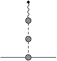
Figure 3: Pion pole graph of the isovector axial-vector current.

Furthermore, $G_{P}(q^{2})$ receives contributions from the pion pole graph of Fig. 3. It consists of three building blocks: The coupling of the external axial source to the pion, the pion propagator, and the ${\pi}N$-vertex, respectively. We consider each part separately.

The renormalized coupling of the external axial source to a pion up to order ${\cal O}(p^{4})$ is given by

$$\epsilon_{A}\cdot qF_{\pi}\delta_{ij},$$ (34)

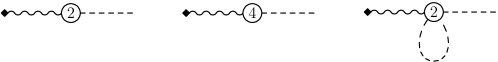
Figure 4: Diagrams contributing to the coupling of the isovector axial-vector current to a pion up to order ${\cal O}(p^{4})$.

where the diagrams in Fig. 4 have been taken into account and the renormalized pion decay constant reads

$$F_{\pi}=F\left[1+\frac{M^{2}}{F^{2}}l_{4}^{r}-\frac{M^{2}}{8\pi^{2}F^{2}}\ln\left(\frac{M}{m}\right)+{\cal O}(M^{4})\right].$$ (35)

We have used the pion wave function renormalization constant

$$Z_{\pi}=1-\frac{2M^{2}}{F^{2}}\left[l_{4}^{r}+\frac{1}{24\pi^{2}}\,\left(R-\ln\left(\frac{M}{m}\right)\right)\right],$$ (36)

with $l_{4}^{r}$ the renormalized coupling of Eq. (17) and $R=\frac{2}{n-4}+\gamma_{E}-1-\ln(4\pi)$.

The renormalized pion propagator is obtained by simply replacing the lowest-order pion mass $M$ by the expression for the physical mass $M_{\pi}$ up to order ${\cal O}(p^{4})$,

$$M^{2}_{\pi}=M^{2}+\Sigma(M^{2}_{\pi})=M^{2}\left[1+\frac{2M^{2}}{F^{2}}\left(l_{3}^{r}+\frac{1}{32\pi^{2}}\ln\left(\frac{M}{m}\right)\right)\right].$$ (37)

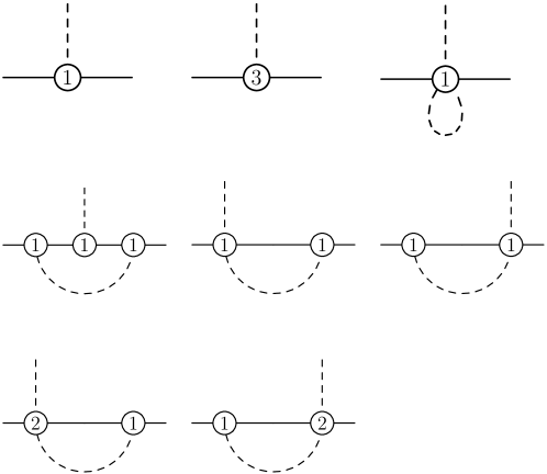
Figure 5: Diagrams contributing to the pion-nucleon vertex up to order ${\cal O}(p^{4})$.

The ${\pi}N$ vertex evaluated between on-mass-shell nucleon states up to order ${\cal O}(p^{4})$ receives contributions from the diagrams in Fig. 5 and the unrenormalized result for a pion with isospin index $i$ is given by

$$\Gamma(q^{2})\gamma_{5}\tau_{i} = \left(-\frac{\texttt{g}_{A}}{F}m_{N}+2\frac{M^{2}}{F}m_{N}(d_{18}-2d_{16})+\frac{\texttt{g}_{A}}{3F^{2}}m_{N}I_{\pi}-2\frac{\texttt{g}_{A}}{F^{3}}M^{2}m_{N}I_{{\pi}N}(m_{N}^{2})\right.$$ (38)

$$-8\frac{\texttt{g}_{A}}{F^{2}}m_{N}^{2}\left\{c_{4}\left[M^{2}I_{{\pi}N}(m_{N}^{2})-I_{{\pi}N}^{(00)}(m_{N}^{2})\right]-c_{3}I_{{\pi}N}^{(00)}(m_{N}^{2})\right\}$$

$$\left.+\frac{\texttt{g}_{A}^{3}}{4F^{3}}m_{N}\left[I_{\pi}+4mN^{2}I_{NN}(q^{2})+4m_{N}^{2}M^{2}I_{{\pi}NN}(q^{2})\right]\right)\gamma_{5}\tau_{i}\,.$$

To find the renormalized vertex one multiplies with $Z\sqrt{Z_{\pi}}$ and replaces the integrals with their infrared singular parts. However, the renormalized result should not be confused with the pion-nucleon form factor $G_{\pi N}(q^{2})$ of Eq. (9). In general, the pion-nucleon vertex depends on the choice of the field variables in the (effective) Lagrangian. In the present case, the pion-nucleon vertex is only an auxiliary quantity, whereas the “fundamental” quantity (entering chiral Ward identities) is the matrix element of the pseudoscalar density. Only at $q^{2}=M_{\pi}^{2}$, we expect the same coupling strength, since both $\hat{m}P^{a}(x)/(M_{\pi}^{2}F_{\pi})$ and the field $\phi_{i}$ of Eq. (12) serve as interpolating pion fields. After renormalization, we obtain for the pion-nucleon coupling constant the quark-mass expansion

$$g_{\pi N}=\texttt{g}_{\pi N}+g_{{\pi}N}^{(1)}M^{2}+g_{{\pi}N}^{(2)}M^{2}\ln\left(\frac{M}{m}\right)+g_{{\pi}N}^{(3)}M^{3}+{\cal O}(M^{4})\,,$$ (39)

with

$$\texttt{g}_{\pi N} = \frac{\texttt{g}_{A}m}{F}\,,$$

$$g_{{\pi}N}^{(1)} = -\texttt{g}_{A}\frac{l_{4}^{r}m}{F^{3}}-4\texttt{g}_{A}\frac{c_{1}}{F}+\frac{2(2d_{16}-d_{18})m}{F}-\texttt{g}_{A}^{3}\frac{m}{16\pi^{2}F^{3}}\,,$$

$$g_{{\pi}N}^{(2)} = -\texttt{g}_{A}^{3}\frac{m}{4\pi^{2}F^{3}}\,,$$

$$g_{{\pi}N}^{(3)} = \texttt{g}_{A}\frac{4+\texttt{g}_{A}^{2}}{32\pi F^{3}}-\texttt{g}_{A}\frac{(c_{3}-2c_{4})m}{6\pi F^{3}}\,,$$ (40)

where all coefficients are understood as IR renormalized parameters. These results agree with the chiral coefficients obtained in Becher:2001hv . In the chiral limit, Eq. (39) satisfies the Goldberger-Treiman relation $\texttt{g}_{\pi N}=\texttt{g}_{A}m/F$ GT . The numerical violation of the Goldberger-Treiman relation as expressed in the so-called Goldberger-Treiman discrepancy Pagels:1969ne ,

$$\Delta=1-\frac{m_{N}g_{A}}{F_{\pi}g_{\pi N}},$$ (41)

is at the percent level, $\Delta=(2.44^{+0.89}_{-0.51})$ % for $m_{N}=(m_{p}+m_{n})/2=938.92$ MeV, $g_{A}=1.2695(29)$, $F_{\pi}=92.42(26)$ MeV, and $g_{\pi N}=13.21^{+0.11}_{-0.05}$ Schroder:rc . Using different values for the pion-nucleon coupling constant such as $g_{\pi N}=13.0\pm 0.1$ Stoks:1992ja , $g_{\pi N}=13.3\pm 0.1$ Ericson:2000md , and $g_{\pi N}=13.15\pm 0.01$ Arndt:2006bf results in the GT discrepancies $\Delta=(0.79\pm 0.84)$ %, $\Delta=(3.03\pm 0.81)$ %, and $\Delta=(1.922\pm 0.363)$ %, respectively. The chiral expansions of $g_{A}$ etc. may be used to relate the parameter $d_{18}$ to $\Delta$ Becher:2001hv ,

$$\Delta=-\frac{2d_{18}M^{2}}{\texttt{g}_{A}}+{\cal O}(M^{4}).$$ (42)

Note that $\Delta$ of Eq. (41) and $\Delta_{GT}$ of Becher:2001hv ; Schroder:rc are related by $\Delta_{GT}=\Delta/(1-\Delta)$. In particular, the leading order of the quark mass expansions of $\Delta$ and $\Delta_{GT}$ is the same.

The induced pseudoscalar form factor $G_{P}(q^{2})$ is obtained by combining Eqs. (33), (35), (37) and the renormalized expression for Eq. (38). With the help of Eqs. (41) and (42) it can entirely be written in terms of known physical quantities as Bernard:1994wn

$$G_{P}(q^{2})=-4\frac{m_{N}F_{\pi}g_{{\pi}N}}{q^{2}-M^{2}_{\pi}}-\frac{2}{3}m_{N}^{2}g_{A}\langle r_{A}^{2}\rangle+{\cal O}(p^{2}).$$ (43)

The $1/(q^{2}-M_{\pi}^{2})$ behavior of $G_{P}$ is not in conflict with the book-keeping of a calculation at chiral order ${\cal O}(p^{4})$, because the external axial-vector field $a_{\mu}$ counts as ${\cal O}(p)$, and the definition of the matrix element contains a momentum $(p^{\prime}-p)^{\mu}$ and the Dirac matrix $\gamma_{5}$ so that the combined order of all ingredients in the matrix element ranges from ${\cal O}(p)$ to ${\cal O}(p^{4})$. The terms that have been neglected in the form factor $G_{P}$ are of order $M^{2}$, $q^{2}/m^{2}$ and higher.

Using the above values for $m_{N}$, $g_{A}$, $F_{\pi}$ as well as $g_{{\pi}N}=13.21^{+0.11}_{-0.05}$, $M_{A}=(1.026\pm 0.021)$ GeV, $M=M_{\pi^{+}}=139.57$ MeV and $m_{\mu}=105.66$ MeV Yao:2006 we obtain for the induced pseudoscalar coupling

$$g_{P}=8.29^{+0.24}_{-0.13}\pm 0.52,$$ (44)

which is in agreement with the heavy-baryon results $8.44\pm 0.23$ Bernard:1994wn and $8.21\pm 0.09$ Fearing:1997dp , once the differences in the coupling constants used are taken in consideration. The first error given in Eq. (44) stems only from the empirical uncertainties in the quantities of Eq. (43). As an attempt to estimate the error originating in the truncation of the chiral expansion in the baryonic sector we assign a relative error of $0.5^{k}$, where $k$ denotes the diffence between the order that has been neglected and the leading order at which a nonvanishing result appears. Such a (conservative) error is motivated by, e. g., the analysis of the individual terms of Eq. (25) as well as the determination of the LECs $c_{i}$ at ${\cal O}(p^{2})$ and to one-loop accuracy ${\cal O}(p^{3})$ in the heavy-baryon framework Bernard:1997gq . For $g_{P}$ we have thus added a truncation error of 0.52.

Figure 6 shows our result for $G_{P}(q^{2})$ in the momentum transfer region $-0.2\,\mbox{GeV}^{2}\leq Q^{2}\leq 0.2\,\mbox{GeV}^{2}$. One can clearly see the dominant pion pole contribution at $q^{2}\approx M^{2}_{\pi}$ which is also supported by the experimental results of Choi:1993vt .

Using Eq. (10) allows one to also determine the pion-nucleon form factor $G_{\pi N}(q^{2})$ in terms of the results for $G_{A}(q^{2})$ and $G_{P}(q^{2})$. When expressed in terms of physical quantities, it has the particularly simple form

$$G_{\pi N}(q^{2})=\frac{m_{N}g_{A}}{F_{\pi}}+g_{\pi N}\Delta\frac{q^{2}}{M_{\pi}^{2}}+{\cal O}(p^{4}).$$ (45)

We have explicitly verified that the results agree with a direct calculation of $G_{\pi N}(q^{2})$ in terms of a coupling to an external pseudoscalar source. Observe that, with our definition in terms of QCD bilinears, the pion-nucleon form factor is, in general, not proportional to the axial form factor. The relation $G_{\pi N}(q^{2})=m_{N}G_{A}(q^{2})/F_{\pi}$ which is sometimes used in PCAC applications implies a pion-pole dominance for $G_{P}(q^{2})$ of the form $G_{P}(q^{2})=4m_{N}^{2}G_{A}(q^{2})/(M_{\pi}^{2}-q^{2})$. However, as can be seen from Eq. (45), there are deviations at ${\cal O}(p^{2})$ from such a complete pion-pole dominance assumption.

The difference between $G_{\pi N}(q^{2}=M_{\pi}^{2})$ and $G_{\pi N}(q^{2}=0)$ is entirely given in terms of the GT discrepancy Bernard:1995dp

$$G_{\pi N}(M_{\pi}^{2})-G_{\pi N}(0)=g_{\pi N}\Delta.$$ (46)

Parameterizing the form factor in terms of a monopole,

$$G_{\pi N}^{{\rm mono}}(q^{2})=g_{\pi N}\frac{\Lambda^{2}-M^{2}}{\Lambda^{2}-q^{2}}\,,$$ (47)

Eq. (46) translates into a mass parameter $\Lambda=894$ MeV for $\Delta=2.44$ %.

IV.2 Inclusion of the axial-vector meson $a_{1}(1260)$

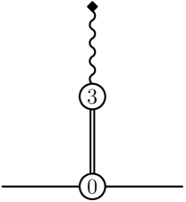
Figure 7: Diagram containing axial-vector meson (double line) contributing to the form factors $G_{A}$ and $G_{P}$.

The contributions of the axial-vector meson to the form factors $G_{A}$ and $G_{P}$ at order ${\cal O}(p^{4})$ stem from the diagram in Fig. 7. We do not consider loop diagrams with internal axial-vector meson lines that do not contain internal pion lines, as these vanish in the infrared renormalization employed in this work. With the Langrangians of Eqs. (21) and (22) the axial form factor receives the contribution

$$G_{A}^{AVM}(q^{2})=-f_{A}g_{a_{1}}\frac{q^{2}}{q^{2}-M_{a_{1}}^{2}}\,,$$ (48)

while the result for the induced pseudoscalar form factor reads

$$G_{P}^{AVM}(t)=4m_{N}^{2}f_{A}g_{a_{1}}\frac{1}{q^{2}-M_{a_{1}}^{2}}\,.$$ (49)

The Lagrangians for the axial-vector meson contain two new LECs, $f_{A}$ and $g_{a_{1}}$, respectively. However, we find that they only appear through the combination $f_{A}g_{a_{1}}$, effectively leaving only one unknown LEC. Performing a fit to the data of $G_{A}(q^{2})$ in the momentum region $0\,\mbox{GeV}^{2}\leq Q^{2}\leq 0.4\,\mbox{GeV}^{2}$ the product of the coupling constants is determined to be

$$f_{A}g_{a_{1}}\approx 8.70.$$ (50)

Fig. 8 shows our fitted result for the axial form factor $G_{A}(q^{2})$ at order ${\cal O}(p^{4})$ in the momentum region $0\,\mbox{GeV}^{2}\leq Q^{2}\leq 0.4\,\mbox{GeV}^{2}$ with the $a_{1}$ meson included as an explicit degree of freedom. As was expected from phenomenological considerations, the description of the data has improved for momentum transfers $Q^{2}\gtrsim 0.1\,\mbox{GeV}^{2}$. We would like to stress again that in a strict chiral expansion up to order ${\cal O}(p^{4})$ the results with and without axial vector mesons do not differ from each other. The improved description of the data in the case with the explicit axial-vector meson is the result of a resummation of certain higher-order terms. While the choice of which additional degree of freedom to include compared to the standard calculation is completely phenomenological, once this choice has been made there exists a systematic framework in which to calculate the corresponding contributions as well as higher-order corrections.

It can be seen from Eq. (48) that in our formalism the axial-vector meson does not contribute to the axial-vector coupling constant $g_{A}$. The pion-nucleon vertex also remains unchanged at the given order, while the axial mean-square radius receives a contribution. The values for the LECs $d_{16}$ and $d_{18}$ therefore do not change, while $d_{22}$ can be determined from the new expression for the axial radius using the value of Eq. (50) for the combination of coupling constants. In Fig. 9 we show the result for $G_{P}(q^{2})$ in the momentum transfer region $-0.2\,\mbox{GeV}^{2}\leq Q^{2}\leq 0.2\,\mbox{GeV}^{2}$. Also shown for comparison is the result without the explicit axial-vector meson. One sees that the contribution of the $a_{1}$ to $G_{P}(q^{2})$ for these momentum transfers is rather small and that $G_{P}(q^{2})$ is still dominated by the pion pole diagrams.

The form factors $G_{A}$ and $G_{P}$ are related to the pion-nucleon form factor via Eq. (10). For the contributions of the axial-vector meson we find

$$2m_{N}G_{A}^{AVM}(q^{2})+\frac{q^{2}}{2m_{N}}G_{P}^{AVM}(q^{2})=0\,,$$ (51)

so that the pion-nucleon form factor is not modified by the inclusion of the $a_{1}$ meson.

V Summary

We have discussed the nucleon form factors $G_{A}$ and $G_{P}$ of the isovector axial-vector current in manifestly Lorentz-invariant baryon chiral perturbation theory up to and including order ${\cal O}(p^{4})$. The main features of the results are similar to the case of the electromagnetic form factors at the one-loop level.

As far as the axial form factor is concerned, ChPT can neither predict the axial-vector coupling constant $g_{A}$ nor the mean-square axial radius $\langle r^{2}_{A}\rangle$. Instead, empirical information on these quantities is used to absorb the relevant LECs $d_{16}$ and $d_{22}$ in $g_{A}$ and $\langle r^{2}_{A}\rangle$. Moreover, the use of a manifestly Lorentz-invariant framework does not lead to an improved description in comparison with the heavy-baryon framework, because the re-summed higher-order contributions are negligible.

The induced pseudoscalar form factor $G_{P}$ is completely fixed from ${\cal O}(p^{-2})$ up to and including ${\cal O}(p)$, once the LEC $d_{18}$ has been expressed in terms of the Goldberger-Treiman discrepancy. Using $g_{\pi N}=13.21$ for the pion-nucleon coupling constant, we obtain for the induced pseudoscalar coupling $g_{P}=8.29^{+0.24}_{-0.13}\pm 0.52$. The first error is due to the error of the empirical quantities entering the expression for $g_{P}$ and the second error represents our estimate for the truncation in the chiral expansion.

Defining the pion field in terms of the PCAC relation allows one to introduce a pion-nucleon form factor which is entirely determined in terms of the axial and induced pseudoscalar form factors. Assuming this pion-nucleon form factor to be proportional to the axial form factor leads to a restriction for $G_{P}$ which is not supported by the most general structure of ChPT.

In addition to the standard treatment including the nucleon and pions, we have also considered the axial-vector meson $a_{1}$ as an explicit degree of freedom. This was achieved by using the reformulated infrared renormalization scheme. The inclusion of the axial-vector meson effectively results in one additional low-energy coupling constant which we have determined by a fit to the data for $G_{A}$. The inclusion of the axial-vector meson results in a considerably improved description of the experimental data for $G_{A}$ for values of $Q^{2}$ up to about $0.4$ GeV², while the contribution to $G_{P}$ is small.

Appendix A Definition of loop integrals

For the definition of the loop integrals in the expressions for the form factors we use the notation

$$P^{\mu}=p_{i}^{\mu}+p_{f}^{\mu},\quad q^{\mu}=p_{f}^{\mu}-p_{i}^{\mu}.$$

Using dimensional regularization 'tHooft:1972fi the loop integrals with one or two internal lines are defined as

$$I_{\pi} = i\int\frac{d^{n}k}{(2\pi)^{n}}\frac{1}{k^{2}-M^{2}+i\epsilon},$$

$$I_{N} = i\int\frac{d^{n}k}{(2\pi)^{n}}\frac{1}{k^{2}-m^{2}+i\epsilon},$$

$$I_{NN}(q^{2}) = i\int\frac{d^{n}k}{(2\pi)^{n}}\frac{1}{[k^{2}-m^{2}+i\epsilon][(k+q)^{2}-m^{2}+i\epsilon]},$$

$$I_{{\pi}N}(p^{2}) = i\int\frac{d^{n}k}{(2\pi)^{n}}\frac{1}{[k^{2}-M^{2}+i\epsilon][(k+p)^{2}-m^{2}+i\epsilon]},$$

$$p^{\mu}I_{{\pi}N}^{(p)}(p^{2}) = i\int\frac{d^{n}k}{(2\pi)^{n}}\frac{k^{\mu}}{[k^{2}-M^{2}+i\epsilon][(k+p)^{2}-m^{2}+i\epsilon]},$$

$$g^{\mu\nu}I_{{\pi}N}^{(00)}(p^{2})+p^{\mu}p^{\nu}I_{{\pi}N}^{(pp)}(p^{2}) = i\int\frac{d^{n}k}{(2\pi)^{n}}\frac{k^{\mu}k^{\nu}}{[k^{2}-M^{2}+i\epsilon][(k+p)^{2}-m^{2}+i\epsilon]}.$$

For integrals with three internal lines we assume on-shell kinematics, $p_{f}^{2}=p_{i}^{2}=m_{N}^{2}$,

$$I_{{\pi}NN}(q^{2}) = i\int\frac{d^{n}k}{(2\pi)^{n}}\frac{1}{[k^{2}-M^{2}+i\epsilon][(k+p_{i})^{2}-m^{2}+i\epsilon][(k+p_{f})^{2}-m^{2}+i\epsilon]},$$

$$P^{\mu}I_{{\pi}NN}^{(P)}(q^{2}) = i\int\frac{d^{n}k}{(2\pi)^{n}}\frac{k^{\mu}}{[k^{2}-M^{2}+i\epsilon][(k+p_{i})^{2}-m^{2}+i\epsilon][(k+p_{f})^{2}-m^{2}+i\epsilon]},$$

$$g^{\mu\nu}I_{{\pi}NN}^{(00)}(q^{2})+P^{\mu}P^{\nu}I_{{\pi}NN}^{(PP)}(q^{2})+q^{\mu}q^{\nu}I_{{\pi}NN}^{(qq)}(q^{2})$$

$$= i\int\frac{d^{n}k}{(2\pi)^{n}}\frac{k^{\mu}k^{\nu}}{[k^{2}-M^{2}+i\epsilon][(k+p_{i})^{2}-m^{2}+i\epsilon][(k+p_{f})^{2}-m^{2}+i\epsilon]}.$$

The tensorial loop integrals can be reduced to scalar ones Passarino:1978jh and we obtain

$$I_{{\pi}N}^{(p)}(p^{2}) = \frac{1}{2p^{2}}\left[I_{\pi}-I_{N}-(p^{2}-m^{2}+M^{2})I_{{\pi}N}(p^{2})\right],$$

$$I_{{\pi}N}^{(00)}(p^{2}) = \frac{1}{2(n-1)}\left[I_{N}+2M^{2}I_{{\pi}N}(p^{2})+\frac{(p^{2}-m^{2}+M^{2})}{p^{2}}I_{\pi N}^{(p)}(p^{2})\right],$$

$$I_{{\pi}NN}^{(P)}(q^{2}) = \frac{1}{4m_{N}^{2}-q^{2}}\left[I_{{\pi}N}(m_{N}^{2})-I_{NN}(q^{2})-M^{2}I_{{\pi}NN}(q^{2})\right],$$

$$I_{{\pi}NN}^{(00)}(q^{2}) = \frac{1}{n-2}\left\{\left[I_{{\pi}NN}(q^{2})+I_{{\pi}NN}^{(P)}(q^{2})\right]M^{2}+\frac{1}{2}I_{NN}(q^{2})\right\},$$

$$I_{{\pi}NN}^{(PP)}(q^{2}) = \frac{1}{(n-2)(4m_{N}^{2}-q^{2})}\left\{\left[(n-1)I_{{\pi}NN}^{(P)}(q^{2})+I_{{\pi}NN}(q^{2})\right]M^{2}\right.$$

$$\left.-\frac{n-2}{2}I_{{\pi}N}^{(p)}(m_{N}^{2})-\frac{n-3}{2}I_{NN}(q^{2})\right\},$$

$$I_{{\pi}NN}^{(qq)}(q^{2}) = -\frac{1}{(n-2)q^{2}}\left\{\left[I_{{\pi}NN}^{(P)}(q^{2})+I_{{\pi}NN}(q^{2})\right]M^{2}+\frac{n-2}{2}I_{{\pi}N}^{(p)}(m_{N}^{2})+\frac{1}{2}I_{NN}(q^{2})\right\}.$$

Defining

$$\bar{\lambda}={m^{n-4}\over 16\pi^{2}}\left\{{1\over n-4}-{1\over 2}\left[\ln(4\pi)+\Gamma^{\prime}(1)+1\right]\right\},$$

and

$$\Omega=\frac{p^{2}-m^{2}-M^{2}}{2mM},$$

the scalar loop integrals are given by Fuchs:2003qc

$$I_{\pi}=2M^{2}\bar{\lambda}+\frac{M^{2}}{8\pi^{2}}\ln\left(\frac{M}{m}\right),$$

$$I_{N}=2m^{2}\bar{\lambda},$$

$$I_{\pi\pi}(q^{2})=2\bar{\lambda}+\frac{1}{16\pi^{2}}\left[1+2\ln\left(\frac{M}{m}\right)+J^{(0)}\left(\frac{q^{2}}{M^{2}}\right)\right],$$

$$I_{NN}(q^{2})=2\bar{\lambda}+\frac{1}{16\pi^{2}}\left[1+J^{(0)}\left(\frac{q^{2}}{m^{2}}\right)\right]$$

$$I_{\pi N}(p^{2})=2\bar{\lambda}+\frac{1}{16\pi^{2}}\left[-1+\frac{p^{2}-m^{2}+M^{2}}{p^{2}}\ln\left(\frac{M}{m}\right)+\frac{2mM}{p^{2}}F(\Omega)\right],$$

where

$$J^{(0)}(x) = \int_{0}^{1}dz\ln[1+x(z^{2}-z)-i\epsilon]$$

$$= \left\{\begin{array}[]{ll}-2-\sigma\ln\left(\frac{\sigma-1}{\sigma+1}\right),&x<0,\\ -2+2\sqrt{\frac{4}{x}-1}\,\mbox{arccot}\left(\sqrt{\frac{4}{x}-1}\right),&0\leq x<4,\\ -2-\sigma\ln\left(\frac{1-\sigma}{1+\sigma}\right)-i\pi\sigma,&4<x,\end{array}\right.$$

with

$$\sigma(x)=\sqrt{1-\frac{4}{x}},\quad x\notin[0,4],$$

and

$$F(\Omega) = \left\{\begin{array}[]{ll}\sqrt{\Omega^{2}-1}\ln\left(-\Omega-\sqrt{\Omega^{2}-1}\right),&\Omega\leq-1,\\ \sqrt{1-\Omega^{2}}\arccos(-\Omega),&-1\leq\Omega\leq 1,\\ \sqrt{\Omega^{2}-1}\ln\left(\Omega+\sqrt{\Omega^{2}-1}\right)-i\pi\sqrt{\Omega^{2}-1},&1\leq\Omega.\end{array}\right.$$

Integrals with three propagators were analyzed numerically using a Schwinger parametrization.

For purely mesonic integrals only the terms proportional to $\bar{\lambda}$ have to be subtracted. To determine the infrared regular parts $R$ of the scalar loop integrals, we use the method described in Schindler:2003xv . On-shell-kinematics are assumed for the subtraction terms. Note that we also list divergent terms, as they might give finite contributions in the expressions for tensor integrals.

$$R_{N} = I_{N},$$

$$R_{NN} = I_{NN},$$

$$R_{\pi N} = \bar{\lambda}\left[2-\frac{M^{2}}{m^{2}}\left(1-8c_{1}m\right)+\frac{3g_{A}^{2}M^{3}}{16\pi F^{2}m}\right]-\frac{1}{16\pi^{2}}-\frac{M^{2}}{32\pi^{2}m^{2}}\left(3+8c_{1}m\right)$$

$$-\frac{3g_{A}^{2}M^{3}}{512\pi^{3}F^{2}m}+{\cal O}(p^{4}),$$

$$R_{\pi NN} = \frac{\bar{\lambda}}{m^{2}}\left[1+\frac{q^{2}}{6m^{2}}+8c_{1}\frac{M^{2}}{m}+\frac{3g_{A}^{2}M^{3}}{16\pi F^{2}m}\right]+\frac{1}{32\pi^{2}m^{2}}-\frac{M^{2}}{32\pi^{2}m^{4}}\left(1-16c_{1}m\right)$$

$$+\frac{3g_{A}^{2}M^{3}}{256\pi^{3}F^{2}m^{3}}+{\cal O}(p^{4}).$$

Figure 2: The axial form factor $G_{A}$ in manifestly Lorentz-invariant ChPT at ${\cal O}(p^{4})$. Full line: result in infrared renormalization with parameters fitted to reproduce the axial mean-square radius corresponding to the dipole parametrization with $M_{A}=1.026$ GeV (dashed line). The dotted and dashed-dotted lines refer to dipole parameterizations with $M_{A}=0.95$ GeV and $M_{A}=1.20$ GeV, respectively. The experimental values are taken from Bernard:2001rs .

Figure 6: The induced pseudoscalar form factor $G_{P}$ in manifestly Lorentz-invariant ChPT at ${\cal O}(p^{4})$.

Figure 8: The axial form factor $G_{A}$ in manifestly Lorentz-invariant ChPT at ${\cal O}(p^{4})$ including the axial-vector meson $a_{1}$ explicitly. Full line: result in infrared renormalization, dashed line: dipole parametrization. The experimental values are taken from Bernard:2001rs .

Figure 9: The induced pseudoscalar form factor $G_{P}$ in manifestly Lorentz-invariant ChPT at ${\cal O}(p^{4})$ including the axial-vector meson $a_{1}$ explicitly. Full line: result with axial-vector meson, dashed line: result without axial-vector meson.

References

- (1) H. y. Gao, Int. J. Mod. Phys. E 12 (2003) 1 [Erratum-ibid. E 12 (2003) 567].
- (2) J. Friedrich and Th. Walcher, Eur. Phys. J. A 17 (2003) 607.
- (3) C. E. Hyde-Wright and K. de Jager, Ann. Rev. Nucl. Part. Sci. 54 (2004) 217.
- (4) V. Bernard, L. Elouadrhiri and U.-G. Meißner, J. Phys. G 28 (2002) R1.
- (5) T. Gorringe and H. W. Fearing, Rev. Mod. Phys. 76 (2004) 31.
- (6) S. L. Adler and F. J. Gilman, Phys. Rev. 152 (1966) 1460.
- (7) S. Scherer and J. H. Koch, Nucl. Phys. A 534 (1991) 461; T. Fuchs and S. Scherer, Phys. Rev. C 68 (2003) 055501.
- (8) J. H. D. Clark et al., Phys. Rev. Lett. 96 (2006) 073401.
- (9) Y. Nambu and E. Shrauner, Phys. Rev. 128 (1962) 862.
- (10) A. Sato, Y. Yokoo and J. Takahashi, Prog. Theor. Phys. 37 (1967) 716.
- (11) R. Tegen and W. Weise, Z. Phys. A 314 (1983) 357.
- (12) W. Y. P. Hwang and D. J. Ernst, Phys. Rev. D 31 (1985) 2884.
- (13) S. Boffi, L. Y. Glozman, W. Klink, W. Plessas, M. Radici and R. F. Wagenbrunn, Eur. Phys. J. A 14 (2002) 17.
- (14) D. Merten, U. Loring, K. Kretzschmar, B. Metsch and H. R. Petry, Eur. Phys. J. A 14 (2002) 477.
- (15) B. Q. Ma, D. Qing and I. Schmidt, Phys. Rev. C 66 (2002) 048201.
- (16) K. Khosonthongkee, V. E. Lyubovitskij, T. Gutsche, A. Faessler, K. Pumsa-ard, S. Cheedket and Y. Yan, J. Phys. G 30 (2004) 793.
- (17) A. Silva, H. C. Kim, D. Urbano and K. Goeke, Phys. Rev. D 72 (2005) 094011.
- (18) K. F. Liu, S. J. Dong, T. Draper, J. M. Wu and W. Wilcox, Phys. Rev. D 49 (1994) 4755; K. F. Liu, S. J. Dong, T. Draper and W. Wilcox, Phys. Rev. Lett. 74 (1995) 2172.
- (19) C. Adamuscin, E. A. Kuraev, E. Tomasi-Gustafsson and F. E. Maas, arXiv:hep-ph/0610429.
- (20) S. Weinberg, Physica A 96 (1979) 327.
- (21) J. Gasser and H. Leutwyler, Annals Phys. 158 (1984) 142.
- (22) J. Gasser and H. Leutwyler, Nucl. Phys. B 250 (1985) 465.
- (23) J. Gasser, M. E. Sainio, and A. Švarc, Nucl. Phys. B307 (1988) 779.
- (24) V. Bernard, N. Kaiser and U.-G. Meißner, Int. J. Mod. Phys. E 4 (1995) 193.
- (25) S. Scherer, in Advances in Nuclear Physics, Vol. 27, edited by J. W. Negele and E. W. Vogt (Kluwer Academic/Plenum Publishers, New York, 2003).
- (26) V. Bernard, N. Kaiser and U.-G. Meißner, Phys. Rev. Lett. 69 (1992) 1877.
- (27) V. Bernard, N. Kaiser, T. S. H. Lee and U.-G. Meißner, Phys. Rept. 246 (1994) 315.
- (28) H. W. Fearing, R. Lewis, N. Mobed and S. Scherer, Phys. Rev. D 56 (1997) 1783.
- (29) V. Bernard, H. W. Fearing, T. R. Hemmert, and U.-G. Meißner, Nucl. Phys. A635 (1998) 121 [Erratum-ibid. A642 (1998) 563].
- (30) S. Weinberg, Phys. Rev. 112 (1958) 1375.
- (31) D. H. Wilkinson, Eur. Phys. J. A 7 (2000) 307.
- (32) K. Minamisono et al., Phys. Rev. C 65 (2002) 015501.
- (33) T. Becher and H. Leutwyler, Eur. Phys. J. C 9 (1999) 643.
- (34) M. R. Schindler, J. Gegelia and S. Scherer, Phys. Lett. B 586 (2004) 258.
- (35) B. Kubis and U.-G. Meißner, Nucl. Phys. A 679 (2001) 698.
- (36) M. R. Schindler, J. Gegelia and S. Scherer, Eur. Phys. J. A 26 (2005) 1.
- (37) W.-M. Yao it et al., J. Phys. G 33 (2006) 1.
- (38) G. Colangelo, J. Gasser and H. Leutwyler, Phys. Rev. Lett. 86 (2001) 5008.
- (39) N. Fettes, U.-G. Meißner, M. Mojzis and S. Steininger, Annals Phys. 283 (2000) 273 [Erratum-ibid. 288 (2001) 249].
- (40) G. Ecker, J. Gasser, H. Leutwyler, A. Pich and E. de Rafael, Phys. Lett. B 223 (1989) 425.
- (41) T. Fuchs, M. R. Schindler, J. Gegelia and S. Scherer, Phys. Lett. B 575 (2003) 11.
- (42) J. Kambor and M. Mojžiš, JHEP 9904 (1999) 031.
- (43) V. Bernard and U. -G. Meißner, Phys. Lett. B 639 (2006) 278.
- (44) S. i. Ando and H. W. Fearing, arXiv:hep-ph/0608195.
- (45) T. Fuchs, J. Gegelia, G. Japaridze and S. Scherer, Phys. Rev. D 68 (2003) 056005.
- (46) A. Liesenfeld et al. [A1 Collaboration], Phys. Lett. B 468 (1999) 20.
- (47) H. Budd, A. Bodek and J. Arrington, Proceedings of the 2nd International Workshop on Neutrino - Nucleus Interactions in the Few GeV Region (NUINT 02), Irvine, California, 12-15 Dec 2002, arXiv:hep-ex/0308005.
- (48) K. S. Kuzmin, V. V. Lyubushkin and V. A. Naumov, Acta Phys. Polon. B 37 (2006) 2337.
- (49) R. Gran et al. [K2K Collaboration], Phys. Rev. D 74 (2006) 052002.
- (50) D. Baumann, PhD Thesis, Johannes Gutenberg-Universität, Mainz (2004).
- (51) T. Fuchs, J. Gegelia and S. Scherer, J. Phys. G 30 (2004) 1407.
- (52) T. Becher and H. Leutwyler, JHEP 0106 (2001) 017.
- (53) M. L. Goldberger and S. B. Treiman, Phys. Rev. 110 (1958) 1178; Phys. Rev. 111 (1958) 354; Y. Nambu, Phys. Rev. Lett. 4 (1960) 380.
- (54) H. Pagels, Phys. Rev. 179 (1969) 1337.
- (55) H. C. Schröder et al., Eur. Phys. J. C 21 (2001) 473.
- (56) V. G. J. Stoks, R. Timmermans and J. J. de Swart, Phys. Rev. C 47 (1993) 512.
- (57) T. E. O. Ericson, B. Loiseau and A. W. Thomas, Phys. Rev. C 66 (2002) 014005.
- (58) R. A. Arndt, W. J. Briscoe, I. I. Strakovsky and R. L. Workman, arXiv:nucl-th/0605082.
- (59) V. Bernard, N. Kaiser and U.-G. Meißner, Phys. Rev. D 50 (1994) 6899.
- (60) V. Bernard, N. Kaiser and U.-G. Meißner, Nucl. Phys. A615 (1997) 483.
- (61) S. Choi et al., Phys. Rev. Lett. 71 (1993) 3927.
- (62) G. ’t Hooft and M. J. G. Veltman, Nucl. Phys. B44 (1972) 189.
- (63) G. Passarino and M. J. G. Veltman, Nucl. Phys. B160 (1979) 151.