Semiclassical Distorted Wave Model Analysis of the $(\pi^{-},K^{+})$ $\Sigma$ Formation Inclusive Spectrum

Abstract

$(\pi^{-},K^{+})$ hyperon production inclusive spectra with $p_{\pi}=1.2$ GeV/c measured at KEK on ¹²C and ²⁸Si are analyzed by the semiclassical distorted wave model. Single-particle wave functions of the target nucleus are treated using Wigner transformation. This method is able to account for the energy and angular dependences of the elementary process in nuclear medium without introducing the factorization approximation frequently employed. Calculations of the $(\pi^{+},K^{+})$ $\Lambda$ formation process, for which there is no free parameter since the $\Lambda$ s.p. potential is known, demonstrate that the present model is useful to describe inclusive spectra. It is shown that in order to account for the experimental data of the $\Sigma^{-}$ formation spectra a repulsive $\Sigma$-nucleus potential is necessary whose magnitude is not so strong as around 100 MeV previously suggested.

I Introduction

Various meson production reactions in nuclei are a rich source of our understanding of hadronic interactions. In particular, interactions involving hyperons have to be explored by strangeness exchange reactions, since hyperons are absent in ordinary nuclear systems. Naturally, the absence itself is a consequence of the properties of strange hadrons. The interaction between the lambda hyperon and the nucleon is fairly well known, since the experimental data for $\Lambda$ hypernuclei has been accumulated in last more than 30 years. The $\Sigma$-$N$ and $\Xi$-$N$ interactions, by contrast, have not been well understood. Even the sign of the $\Sigma$ single-particle (s.p.) potential in nuclear medium, which reflects basic properties of the $\Sigma$-$N$ interaction, has not been established. Interactions among hyperons are far less investigated, except for the $\Lambda\Lambda$ case.

In recent years, much experimental effort has been directed to the study of strange baryons and baryonic resonances in nuclear medium, using incident $\pi$, $K$ and $\gamma$ beams with the energy of 1 $\sim$ 2 GeV. The extraction of meaningful understanding of these baryon properties from such reaction processes is not so simple, however. For analyzing experimental data we need to take into account various effects, such as the proper treatment of projectiles and outgoing hadrons, the model description of elementary processes in nuclei and the decent description of the target nucleus and the residual (hyper) nucleus. We also have to keep in mind the possibility of the change of properties of the relevant hadrons themselves in nuclear medium.

Since fully microscopic description is far from practical, various approximations are commonly introduced to analyze the experimental data. Then, it is important to employ a model as simple and reliable as possible, bearing in mind that lack of some proper treatment can easily lead to misunderstanding of the basic hadron properties.

$\Sigma$ formation spectra in $(\pi,K)$ and $(K,\pi)$ reactions with nuclei are not expected to have narrow peaks, because of the strong $\Sigma N\rightarrow\Lambda N$ coupling. In spite of this, however, the early $(K,\pi)$ experimental spectra BERT were interpreted as indicating an attractive $\Sigma$ s.p. potential with the depth of about 10 MeV KHW ; DMG . The experimental discovery of ${}^{\hskip 0.70004pt4}_{\Sigma}$He HAYA ; NAGA has shown that the $\Sigma$-$N$ interaction in the $T=1/2$ channel is sufficiently attractive to support the bound state in this specific nucleus, as discussed by Harada HARA . It has been recognized, however, that due to the strong repulsion in the isospin $T=3/2$ channel, $\Sigma$ bound states are unlikely to be observed in heavier nuclei. This conjecture was supported by experimental results on targets of ⁶Li and ⁹Be measured at BNL BART . The analysis of the $(K,\pi)$ spectra on ⁹Be from BNL BNL given by Da̧browski DAB in a plane wave impulse approximation method suggested that the $\Sigma$ potential is repulsive of the order of 20 MeV.

The shift and the width of $\Sigma^{-}$ atomic states are another source of the information on the $\Sigma$-nucleus potential. Batty, Friedman and Gal BFG reexamined the $\Sigma^{-}$ atomic data and concluded that the $\Sigma$ potential should be attractive at the surface region but changes its sign to become repulsive at the higher density region in a nucleus.

Theoretical studies for the two-body $\Sigma$-$N$ force have also been inconclusive. In the 1970s, the Nijmegen group started to construct hard-core hyperon-nucleon potentials in a one-boson exchange model. Parameter sets corresponding to two typical choices of the SU(3) mixing angles were named as models D and F NIJDF . The $G$-matrix calculation by Yamamoto and Bando in Ref. YB1 showed that the model D yields $-29.3$ MeV for the $\Sigma$ potential in nuclear matter at the normal density ($k_{F}=1.35$ fm^-1) and the model F repulsive 5.8 MeV, though the explicit numbers vary in a different calculational scheme. The soft-core versions subsequently constructed by the Nijmegen group NIJNS tend to predict an attractive $\Sigma$ s.p. potential in nuclear medium; $-27.1$ MeV in Ref. YB1 and $-15.3$ MeV in the nuclear matter calculation by Schulze et al.SCHU .

A different approach using a non-relativistic SU(6) quark model has been developed by the Kyoto-Niigata group FU96a ; FU96b ; FU01 to obtain a unified description of octet baryon-baryon interactions. In this model, the description of the short-ranged part of baryon-baryon interactions basically provided by the resonating-group method with the spin-flavor SU(6) quark model wave functions and the one-gluon exchange Fermi-Breit interaction is supplemented by effective meson-exchange potentials acting between quarks. This model has little ambiguities in the hyperon-nucleon sector after the nucleon-nucleon interaction is determined. $G$ matrix calculations in the lowest order Brueckner theory KOH with the potential named as FSS FU96a ; FU96b show that the $\Sigma$ s.p. potential in symmetric nuclear matter is repulsive of the order of 20 MeV at normal density. The repulsion due to a strongly repulsive character in the isospin $T=\frac{3}{2}$ ${}^{3}S_{1}$ channel originating from quark Pauli effects overcomes an attractive contribution in the $T=1/2$ ${}^{3}S_{1}$ channel which is similar to that in the $\Lambda N$ case. The latest version of this quark model potential, fss2 FU01 , gives a smaller repulsion of about 8 MeV in symmetric nuclear matter.

We briefly mention relativistic mean filed model description for the hyperon sector. This model does not seem to have much predictive power, but once parameters are determined to fit basic properties it has wide applicability, for example, to a variety of neutron star matter calculations. In early models including only $\sigma$ meson, the $\Sigma$ hyperon is predicted to have the similar attractive potential to the $\Lambda$ in nuclear medium. Having recognized that the $\Sigma$ s.p. potential may be repulsive in nuclei, the model was extended to include $\sigma^{*}$ meson to account for that property. The repulsion of 30 MeV has been tentatively used in literature MFGJ ; SBG , although this specific number did not have a solid basis.

It is also noted that Kaiser KAIS calculated the $\Sigma$ mean-field in symmetric nuclear matter in the framework of SU(3) chiral perturbation theory and found a moderately repulsive potential, that is, 59 MeV for the real part and -21.5 MeV for the imaginary one at normal density.

Recently, inclusive $(\pi^{-},K^{+})$ spectra corresponding to $\Sigma$ formation were measured at KEK KEK ; SAHA with better accuracy than before, using the pion beam with the momentum of $p_{\pi}=1.2$ GeV/c on medium-to heavy nuclear targets. DWIA analyses in Ref. KEK for ²⁸Si and similar analyses later on other nuclear targets SAHA gave a notable conclusion that the $\Sigma$ potential is strongly repulsive, as large as 100 MeV. Harada and Hirabayashi HH showed in similar calculations with their optimal Fermi-averaging for the elementary $t$-matrix that the $\Sigma$ potential is repulsive inside the nuclear surface, though the actual strength varies with the imaginary part supposed.

The determination of the $\Sigma$-$N$ interaction is of fundamental importance in the study of such problems as those of neutron star matter and heavy ion collisions, because the baryonic component of such hadronic matter, especially the hyperon admixture, is governed by the basic baryon-baryon interactions. Considering the importance of determining the $\Sigma$-$N$ interaction on the basis of experimental data, it is desirable to analyze the KEK experiments in a different and independent calculational scheme from those in Refs. KEK ; HH . In this paper, we present a semiclassical method for the DWIA approach and apply it to $(\pi^{\pm},K^{+})$ inclusive spectra. The preparatory version of this approach was reported in Ref. MK . The semiclassical distorted wave (SCDW) model was originally considered for describing intermediate energy nucleon inelastic reactions on nuclei SCDW1 . Applications to various $(p,p^{\prime})$ and $(p,n)$ inclusive spectra SCDW2 ; SCDW3 have demonstrated that the method is quantitatively reliable and thus the applications to the wide range of nuclear reactions are promising.

In Sec. II, we show basic expressions of the semiclassical distorted wave model for describing the $(\pi,K)$ inclusive spectra. The formulation using the Wigner transformation for the nuclear density matrix is explained. Actual optical potential model parameters used for incident pions and outgoing kaons are given in Sec. III. Then, numerical results for the $(\pi^{\pm},K^{+})$ spectra are presented in Sec. IV: first for the $\Lambda$ formation to see the applicability of the SCDW model and next for the $\Sigma$ formation. The latter case is the main concern of the present paper to obtain more solid information about the strength of the $\Sigma$ single-particle potential than before. In this paper, we are concerned with the spectra on light nuclei with $N=Z$, namely ²⁸Si and ¹²C. Conclusions are given in Sec. V, with the outlook of the future extension of our model.

II Semiclassical distorted wave model description of the $(\pi,K)$ inclusive spectra

The starting formula for the double differential cross section in a standard distorted wave model description of the $(\pi,K)$ hyperon ($Y$) production inclusive reaction is expressed as

$$\frac{d^{2}\sigma}{dWd\Omega} = \frac{\omega_{i}\omega_{f}}{(2\pi)^{2}}\frac{p_{f}}{p_{i}}\int\int d\mbox{\boldmath$r$}d\mbox{\boldmath$r$}^{\prime}\sum_{p,h}\;\frac{1}{4\omega_{i}\omega_{f}}\chi_{f}^{(-)*}(\mbox{\boldmath$r$})v_{f,p,i,h}\chi_{i}^{(+)}(\mbox{\boldmath$r$})\chi_{f}^{(-)}(\mbox{\boldmath$r$}^{\prime})v^{*}_{f,p,i,h}\chi_{i}^{(+)*}(\mbox{\boldmath$r$}^{\prime})$$ (1)

$$\times\phi_{p}^{*}(\mbox{\boldmath$r$})\phi_{h}(\mbox{\boldmath$r$})\phi_{p}(\mbox{\boldmath$r$}^{\prime})\phi_{h}^{*}(\mbox{\boldmath$r$}^{\prime})\delta(W-\epsilon_{p}+\epsilon_{h})\theta(\epsilon_{F}-\epsilon_{h}),$$

where $\chi_{i}^{(+)}$ and $\chi_{f}^{(-)}$ represent the incident pion and final kaon wave functions with energies $\omega_{i}$ and $\omega_{f}$, respectively, and $W=\omega_{i}-\omega_{f}$ is the energy transfer. The formula describes the process in which the nucleon in the occupied single-particle state $h$ is converted to the unobserved outgoing hyperon ($\Lambda$ or $\Sigma$) state $p$. The elementary amplitude of the process $\pi+N\rightarrow K+Y$ is denoted by $v_{f,p,i,h}$, which depends on the energy and momentum of the particles in the reaction. In order to treat such dependence, it is necessary to introduce momentum space integration. In that case, the explicit calculations involve higher-dimensional integrations. It is desirable, in practice, to develop a tractable and trustful approximation method. One procedure that has been frequently used is the factorization approximation, in which the elementary process is taken out of the integration, assuming some averaging wisdom. As used in Ref. KEK for $\pi^{-}+p\rightarrow K^{+}+\Sigma^{-}$, the elementary amplitude in the integrand may be replaced by the averaged differential cross section over the nucleon momentum distribution $\rho(\mbox{\boldmath$k$})$,

$$\overline{\frac{d\sigma(\pi^{-}p\rightarrow K^{+}\Sigma^{-})}{d\Omega}}\equiv\frac{\int\rho(\mbox{\boldmath$k$})\frac{d\sigma}{d\Omega}(\Omega_{k})\delta(k-P)dk}{\int\rho(\mbox{\boldmath$k$})\delta(k-P)dk}$$ (2)

with $P=k_{K}+k_{Y}-k_{\pi}$, and is taken outside of the integration. The remaining quantity is the Green function, which is not difficult to evaluate in the case of a local optical potential. A more sophisticated Fermi-averaging method was used in Ref. HH . Though such procedure has been widely applied to show various successes, the justification is far from trivial. Important dynamical effects might be hidden in the averaging treatment.

II.1 SCDW method

In Ref. MK , we presented our SCDW approximation method for the DWIA cross section formula, Eq. (1). There, we introduced a local Fermi gas approximation for the target nucleus. In this paper, we improve the description by explicitly treating s.p. wave functions of the target nucleus.

The semiclassical treatment was first introduced in the description of the intermediate energy nucleon reactions on nuclei SCDW1 . Since the amount of numerical calculations is reduced, it becomes feasible to include and assess multi-step contributions. The calculations of $(p,p)$ and $(p,n)$ inclusive spectra have shown that the SCDW method works well.

The semiclassical approximation employs the following idea for the propagation of the wave function. Denoting the midpoint and the relative coordinates of $r$ and $\mbox{\boldmath$r$}^{\prime}$ in Eq. (1) by $\mbox{\boldmath$R$}=\frac{\mbox{\boldmath$r$}+\mbox{\boldmath$r$}^{\prime}}{2}$ and $\mbox{\boldmath$s$}=\mbox{\boldmath$r$}^{\prime}-\mbox{\boldmath$r$}$, respectively, we assume that the propagation of the distorted waves, $\chi_{i}$ and $\chi_{f}$, from $R$ to $r$ or $\mbox{\boldmath$r$}^{\prime}$ is described by a plane wave with the local classical momentum $\mbox{\boldmath$k$}(\mbox{\boldmath$R$})$ at the position $R$.

$$\chi_{i}^{(+)}\left(\mbox{\boldmath$R$}\pm\frac{1}{2}\mbox{\boldmath$s$}\right) \simeq \mbox{e}^{\pm i\frac{1}{2}\mbox{\boldmath$s$}\cdot\mbox{\boldmath$k$}_{i}(\mbox{\boldmath$R$})}\chi_{i}^{(+)}(\mbox{\boldmath$R$}),$$ (3)

$$\chi_{f}^{(-)}\left(\mbox{\boldmath$R$}\pm\frac{1}{2}\mbox{\boldmath$s$}\right) \simeq \mbox{e}^{\pm i\frac{1}{2}\mbox{\boldmath$s$}\cdot\mbox{\boldmath$k$}_{f}(\mbox{\boldmath$R$})}\chi_{f}^{(-)}(\mbox{\boldmath$R$}).$$ (4)

The local momentum $\mbox{\boldmath$k$}(\mbox{\boldmath$R$})$ is defined as follows. The direction is specified by the quantum mechanical momentum density $\mbox{\boldmath$k$}_{q}(\mbox{\boldmath$R$})$ calculated by

$$\mbox{\boldmath$k$}_{q}(\mbox{\boldmath$R$})=\frac{\Re\{\chi^{(\pm)*}(\mbox{\boldmath$R$})(-i)\nabla\chi^{(\pm)}(\mbox{\boldmath$R$})\}}{|\chi^{(\pm)}(\mbox{\boldmath$R$})|^{2}},$$ (5)

where $\Re$ represents taking the real part, and the magnitude is determined by the energy-momentum relation $\frac{\hbar^{2}}{2\mu}k^{2}(\mbox{\boldmath$R$})+U_{R}(\mbox{\boldmath$R$})=E$ at $R$. Here, $U_{R}(\mbox{\boldmath$R$})$ is the real part of an optical potential for the distorted wave function $\chi$ with energy $E$. The relativistic energy-momentum relation is used for the distorted wave function described by the Klein-Gordon equation.

The above approximation is expected to work well if the dominant contributions in the integration over $r$ and $\mbox{\boldmath$r$}^{\prime}$ in Eq. (1) is restricted in the region where $r$ and $\mbox{\boldmath$r$}^{\prime}$ are close to each other. Actually, the density matrix $\sum_{h}\phi_{h}^{*}(\mbox{\boldmath$r$}^{\prime})\phi_{h}(\mbox{\boldmath$r$})$ brings about this desirable feature, as is shown in the following heuristic argument. It is sufficient for the qualitative discussion to assume that nuclear s.p. wave functions are harmonic oscillator ones. The summation over the $z$-component of the angular momentum of each orbit means that we are treating two oscillator functions coupled to the total angular momentum $L=0$;

$$\sum_{m_{h}}\;\phi_{h}^{*}(\mbox{\boldmath$r$}_{1})\phi_{h}(\mbox{\boldmath$r$}_{2})$$ (6)

$$\rightarrow \sqrt{2\ell_{h}+1}|n_{h}\ell_{h}(\mbox{\boldmath$r$}_{1}),n_{h}\ell_{h}(\mbox{\boldmath$r$}_{2});L=0\rangle.$$

The transformation to the $R$ and $s$ coordinates are carried out using the Talmi-Moshinsky brackets.

$$|n_{h}\ell_{h}(\mbox{\boldmath$r$}_{1}),n_{h}\ell_{h}(\mbox{\boldmath$r$}_{2});L=0\rangle=\hskip 85.35826pt$$

$$\sum_{N,n,\ell}\langle n\ell,N\ell;0|n_{h}\ell_{h},n_{h}\ell_{h};0\rangle|n\ell(\mbox{\boldmath$s$}),N\ell(\mbox{\boldmath$R$});L=0\rangle.$$ (7)

The reaction processes which we consider take place mostly at the surface of the target nucleus. When $R$ is located in the surface region, the dominant components in the right hand side of Eq. (7) are those in which $2N+\ell$ is the largest. This indicates that the dependence on the relative coordinate $s$ is governed by the $0s$ ($n=0$ and $\ell=0$) function, which is certainly short-ranged compared with the size of the target nucleus. Thus we expect that the SCDW treatment of Eqs. (3,4) in Eq. (1) is meaningful.

Note that since the SCDW approximation should be exact in homogeneous matter, the SCDW works well inside of the nucleus. The above reasoning implies that the SCDW approximation is also applicable to the surface region. This fact is probably connected to the fact that the local density approximation based on the density matrix expansion method NV works well in nuclear structure calculations, including the surface region.

II.2 Wigner transformation

In the preparatory calculations in Ref. MK , we introduced a Thomas-Fermi approximation for the density matrix $\sum_{h}\;\phi_{h}^{*}(\mbox{\boldmath$r$}^{\prime})\phi_{h}(\mbox{\boldmath$r$})$ of the target nucleus. Here, we elaborate the description of the density matrix by using a Wigner transformation.

The Wigner transformation of the density matrix of the target nuclear wave function is defined as

$$\sum_{h}\;\phi_{h}^{*}(\mbox{\boldmath$r$}^{\prime})\phi_{h}(\mbox{\boldmath$r$}) = \sum_{h}\phi^{*}_{h}\left(\mbox{\boldmath$R$}-\frac{1}{2}\mbox{\boldmath$s$}\right)\phi_{h}\left(\mbox{\boldmath$R$}+\frac{1}{2}\mbox{\boldmath$s$}\right)$$ (8)

$$= \int d\mbox{\boldmath$K$}\;\sum_{h}\Phi_{h}(\mbox{\boldmath$R$},\mbox{\boldmath$K$})\;e^{i\mbox{\boldmath$K$}\cdot\mbox{\boldmath$s$}}.$$

$\Phi_{h}(\mbox{\boldmath$R$},\mbox{\boldmath$K$})$ is given by the inverse transformation as

$$\Phi_{h}(\mbox{\boldmath$R$},\mbox{\boldmath$K$}) \equiv \frac{1}{(2\pi)^{3}}\int d\mbox{\boldmath$s$}\;e^{-i\mbox{\boldmath$s$}\cdot\mbox{\boldmath$K$}}$$ (9)

$$\times\;\phi_{h}^{*}(\mbox{\boldmath$R$}-\frac{1}{2}\mbox{\boldmath$s$})\phi_{h}(\mbox{\boldmath$R$}+\frac{1}{2}\mbox{\boldmath$s$}).$$

The summation over the $z$-component of the angular momentum is implicit in these expressions. As is shown in the Appendix, $\Phi_{h}(\mbox{\boldmath$R$},\mbox{\boldmath$K$})$ may be expressed in terms of the Legendre expansion:

$$\Phi_{h}(\mbox{\boldmath$R$},\mbox{\boldmath$K$})=\sum_{\ell=\mbox{even}}P_{\ell}(\cos\widehat{\mbox{\boldmath$K$}\mbox{\boldmath$R$}})\;\Phi_{h}^{\ell}(R,K),$$ (10)

where $\widehat{\mbox{\boldmath$K$}\mbox{\boldmath$R$}}$ denotes the angle between two vectors $K$ and $R$. It is easy to see that the Thomas-Fermi approximation for the density matrix used in Ref. MK amounts to the replacement

$$\sum_{h}\sum_{\ell}P_{\ell}(\cos\widehat{\mbox{\boldmath$K$}\mbox{\boldmath$R$}})\;\Phi_{h}^{\ell}(R,K)$$

$$\rightarrow\frac{2}{(2\pi)^{3}}\theta(k_{F}(R)-K),$$ (11)

where $\theta(x)$ is a step function and $k_{F}(R)=[3\pi^{2}\rho_{\tau}(R)]^{1/3}$ is a local Fermi momentum determined by the local proton or neutron density $\rho_{\tau}(R)$ at $R$.

We describe unobserved hyperons by a local optical potential. Actually, the hyperon optical potential should be complex, because there are inelastic processes. The standard way to treat the completeness of the final states described by a complex Hamiltonian is to use the Green function method HLM . At this stage, however, we adopt a simplified prescription, employing a real potential of the standard Woods-Saxon form,

$$U_{Y}(r)=U_{Y}^{0}/\{1+\exp((r-r_{0})/a)\},$$ (12)

and we convolute the result of the calculated spectrum with a Lorentz-type distribution function with the typical width, simulating the effects of inelastic channels. In that case, the expression of Eq. (1) is directly used. Then, we introduce the SCDW approximation as in Eqs. (3,4) also for the hyperon wave functions $\phi_{p}(\mbox{\boldmath$r$})$ and $\phi_{p}(\mbox{\boldmath$r$}^{\prime})$.

Using these approximations explained above, the double differential cross section in the SCDW model becomes

$$\displaystyle\frac{d^{2}\sigma}{dWd\Omega} = \frac{\omega_{i}\omega_{f}}{(2\pi)^{2}}\frac{p_{f}}{p_{i}}\int d\mbox{\boldmath$R$}\int d\mbox{\boldmath$K$}\;\sum_{p}\;\frac{1}{4\omega_{i}\omega_{f}}|\chi_{f}^{(-)}(\mbox{\boldmath$R$})|^{2}|\chi_{i}^{(+)}(\mbox{\boldmath$R$})|^{2}|\phi_{p}(\mbox{\boldmath$R$})|^{2}(2\pi)^{3}\sum_{h}\sum_{\ell}P_{\ell}(\cos\widehat{\mbox{\boldmath$K$}\mbox{\boldmath$R$}})\;\Phi_{h}^{\ell}(R,K)$$ (13)

$$\times|v_{f,p,i,h}(\mbox{\boldmath$K$},\mbox{\boldmath$k$}_{i})|^{2}\delta(\mbox{\boldmath$K$}+\mbox{\boldmath$k$}_{i}(\mbox{\boldmath$R$})-\mbox{\boldmath$k$}_{f}(\mbox{\boldmath$R$})-\mbox{\boldmath$k$}_{p}(\mbox{\boldmath$R$}))\;\delta(W-\epsilon_{p}+\epsilon_{h}).$$

The summation $\sum_{p}$ means the sum over the spin and the momentum of the outgoing unobserved hyperon: $\frac{1}{(2\pi)^{3}}\sum_{\mbox{spin}}\int\>d\mbox{\boldmath$p$}$. If we use the energy, instead of the momentum, to specify scattering states, the momentum integration $\int\>d\mbox{\boldmath$p$}$ is written as follows:

$$\int\;d\Omega_{p}\int\frac{1}{2}\left(\frac{2m_{Y}}{\hbar^{2}}\right)^{3/2}\sqrt{\epsilon_{p}}\;d\epsilon_{p}.$$ (14)

The above final expression (13) admits of the simple interpretation that the reaction in which $\pi+N$ yields $K+Y$ takes place at the position $R$ and satisfies conservation of local semiclassical momentum:

$$\mbox{\boldmath$K$}+\mbox{\boldmath$k$}_{i}(\mbox{\boldmath$R$})=\mbox{\boldmath$k$}_{f}(\mbox{\boldmath$R$})+\mbox{\boldmath$k$}_{p}(\mbox{\boldmath$R$})$$ (15)

These momenta, $\mbox{\boldmath$k$}_{i}(\mbox{\boldmath$R$})$, $\mbox{\boldmath$k$}_{f}(\mbox{\boldmath$R$})$ and $\mbox{\boldmath$k$}_{p}(\mbox{\boldmath$R$})$, are calculated with Eq. (5), using $\pi$, $K$ and $Y$ distorted wave functions in an optical model description. It is seen that the dimension of the integration does not change from Eq. (1) to Eq. (13). However, we can now treat the momentum dependence of the transition amplitude $v_{f,p,i,h}$ explicitly.

In the present formulation, the correction for the lack of the translational invariance ES in the target nuclear wave function is not included. In describing electron scattering on a nucleus composed of $A$ nucleons, the center-of-mass effects TB in the nuclear shell model have been taken care of by a multiplicative factor $F^{1/2}=\exp(q^{2}/(4A\alpha))$, where $q$ is the momentum transfer and $\alpha$ is the oscillator constant. For $A=12$ and $\alpha=0.4$ fm^-2, the factor $|F^{1/2}|^{2}$ amounts to 1.5 when the momentum transfer is 2 fm^-1. Thus the calculation without the center-of-mass correction tends to underestimate the cross section. The appropriate treatment of the center-of-mass effects in our SCDW method deserves to be studied in the future.

II.3 Elementary amplitude

The on-shell amplitude $v_{f,p,i,h}$ of the elementary process is related to the differential cross section by

$$\frac{d\sigma}{d\Omega}=\frac{1}{(4\pi)^{2}}\frac{E_{N}E_{Y}}{s}\frac{k_{K}}{k_{\pi}}|v|^{2},$$ (16)

where $s$ is the invariant mass squared. In Eq. (13), we are able to account for the angular dependence of the $\pi+N\rightarrow K+Y$ elementary process at each position $R$. To carry out an actual calculation in Eq. (13), we need some model description for $v$. However, at present, there is no reliable model for the relevant process, including off-shell regions. We use a simple phenomenological parametrization based on Eq. (16), by defining the invariant mass squared using the momenta $\mbox{\boldmath$k$}_{i}(\mbox{\boldmath$R$})$ and $K$. The following functional form is used to simulate empirical angular distributions of the $\pi+N\rightarrow K+Y$ reactions.

$$\frac{d\sigma}{d\Omega}=\frac{\sigma(\sqrt{s})}{4\pi}\{1+\sum_{\ell}a_{\ell}(\sqrt{s})P_{\ell}(\cos\theta)\}$$ (17)

Values of $\sigma(\sqrt{s})$ and $a_{\ell}(\sqrt{s})$ used in the present calculations will be given in Sec. IV.

II.4 Wave functions of the target nucleus and hyperons

In this paper, we are concerned with the reactions on the $N=Z$ targets, ²⁸Si and ¹²C. Single-particle wave functions and the energies for these nuclei $\epsilon_{h}$ are prepared by the density-dependent Hartree-Fock description of Campi-Sprung CS .

As stated in B of this section, hyperons are described by an energy-independent local potential of the Woods-Saxon form. We use the standard geometry parameters, $r_{0}=1.25\times(A-1)^{1/3}$ fm and $a=0.65$ fm. The Coulomb potential regularized in a nucleus is incorporated in the case of the $\Sigma^{-}$. It is noted that if we use a different parameter set such as $r_{0}=1.20\times(A-1)^{1/3}$ fm and $a=0.6$ fm, we do not see appreciable changes in calculated spectra for ¹²C and ²⁸Si.

It may be argued that the hyperon s.p. potential is not expressed by a single Woods-Saxon shape. The $\Sigma$ potential may be repulsive in the higher density region, but change its sign at the surface as has been suggested by the analysis BFG of $\Sigma^{-}$ atomic data and also by the nuclear matter calculations KOH with the SU(6) quark model interaction. At present, however, it is premature to discuss the detailed shape of the $\Sigma$ potential from the available inclusive spectra. We assume, from the beginning, the standard Woods-Saxon form and ask what strength $U_{\Sigma}^{0}$ is favored by the experimental data. More experimental data is needed to quantitatively discuss more elaborate shape parameters as well as the possible energy-dependence of the strength.

The nuclear matter calculations KOH with the SU(6) quark model interaction suggest that the imaginary strength of the $\Lambda$ s.p. potential hardly depends on the density, but that of the $\Sigma$ s.p. potential decreases when the nuclear matter density becomes lower. Regarding that the hyperon formation processes take places at the surface region, we set the energy dependence of the half width in MeV for smearing the calculated spectra as follows, simulating the calculated results at the half of the normal density with the quark model potential FSS:

$$\frac{\Gamma_{\Lambda}(E)}{2} = \left\{\begin{array}[]{l}1+12(E/40)^{2}-8(E/40)^{3},\hskip 5.0ptE\leq 40\mbox{ MeV}\\ \\ 5,\hskip 10.00002ptE>40\mbox{ MeV},\end{array}\right.$$ (21)

$$\frac{\Gamma_{\Sigma}(E)}{2} = 10+\frac{10}{1+(20/E)^{2}},\hskip 5.0pt\mbox{$E$ in MeV}.$$ (22)

III Optical potentials for pions and kaons

Figure 1: Differential cross section of $\pi^{+}$ elastic scattering on ¹²C at $p_{\pi}=800$ MeV/c. Calculated values in the optical potential model with $-ib_{0}=1.0$ fm³ is compared with the experimental data CPI .

The incident pions and detected kaons are described by the standard Klein-Gordon equation with some optical potential model. Following the usual procedure to construct a $\pi$-nucleus optical potential from $\pi N$ elementary amplitudes, the optical potential for the pion is given by

$$V_{\pi}(r)=-\frac{k^{2}}{2E_{\pi}}b_{0}\rho(r)$$ (23)

where $\rho(r)$ is the one-body nuclear density distribution and the parameter $b_{0}$ is related to the sum of isospin averaged $\pi N$ partial wave amplitudes. In practice, a pure imaginary choice of $b_{0}=i\frac{1}{k}\langle\sigma_{tot}\rangle$ is found to work well. As an example, we show, in Fig. 1, the pion elastic scattering differential cross sections on ¹²C at 800 MeV/c. We simply expect at the present stage that the same prescription is applicable to the incident momentum of 1.2 GeV/c. Actually, $-ib_{0}=0.58$ fm³ at 1.2 GeV/c and $-ib_{0}=0.70$ fm³ at 1.05 GeV/c.

Figure 2: Differential cross section of $K^{+}$ elastic scattering on ¹²C at $p_{K}=800$ MeV/c. The optical model with the parameter $b_{0}$ given in Eq. (21) gives the result shown by a solid curve, compared with the experimental data MAR .

Figure 3: Differential cross section of $K^{+}$ elastic scattering on ¹²C at $p_{K}=715$ MeV/c. The optical model with the parameter $b_{0}$ given in Eq. (21) gives the result shown by a solid curve, compared with the experimental data MIC .

It has been known SKG that the kaon scattering data is not well reproduced by simply folding elementary amplitudes. In the present calculation, we phenomenologically search an optimal parameter $b_{0}$ in the form of Eq. (20), using the available experimental data MAR ; MIC on C at 800 MeV/c and 715 MeV/c. For the K⁺, we find that the following momentum dependence is adequate;

$$b_{0}=-6.2\times 10^{-4}p_{K}+i\frac{90.0}{p_{K}},$$ (24)

where $b_{0}$ in fm³ and $p_{K}$ in MeV/c. As shown in Figs. 2 and 3, the calculated differential cross sections account well for the experimental data. The outgoing $K^{+}$ momenta relevant to the present inclusive spectra are in this energy region.

Table 1: Legendre coefficients $a_{\ell}(\sqrt{s})$ in Eq. (17) of the differential cross sections of the $\pi^{-}+p\rightarrow K^{0}+\Lambda$ reaction, determined using experimental data BAK ; SAX .

	$a_{\ell}$		range of $\sqrt{s}$ (GeV)
$\ell=1$	$12.6\sqrt{s}-20.362$		$\sqrt{s}\leq 1.69$
	$0.932$		$1.69<\sqrt{s}\leq 1.925$
	$-4.8\sqrt{s}+10.172$		$1.925<\sqrt{s}\leq 2.015$
	$2.164\sqrt{s}-3.86$		$2.015<\sqrt{s}\leq 2.3$
$\ell=2$	$0$		$\sqrt{s}\leq 1.677$
	$11.82\sqrt{s}-19.821$		$1.677<\sqrt{s}\leq 1.7$
	$0.273$		$1.7<\sqrt{s}\leq 1.8$
	$4.71\sqrt{s}-8.205$		$1.8<\sqrt{s}\leq 2.4$
$\ell=3$	$0$		$\sqrt{s}\leq 1.8$
	$-5.68\sqrt{s}+10.224$		$1.8<\sqrt{s}\leq 1.85$
	$-0.284$		$1.85<\sqrt{s}\leq 1.98$
	$-8.32\sqrt{s}+16.19$		$1.98<\sqrt{s}\leq 2.03$
	$6.13\sqrt{s}-13.144$		$2.03<\sqrt{s}\leq 2.4$
$\ell=4$	$0$		$\sqrt{s}\leq 1.86$
	$7.5\sqrt{s}-13.95$		$1.86<\sqrt{s}\leq 1.96$
	$0.75$		$1.96<\sqrt{s}\leq 2.08$
	$5.5\sqrt{s}-10.69$		$2.08<\sqrt{s}\leq 2.4$

IV Results

IV.1 $\Lambda$ formation

We first apply our SCDW model to the $(\pi^{+},K^{+})$ $\Lambda$ formation inclusive spectra obtained with ²⁸Si and ¹²C targets measured at KEK SAHA ; SAHA2 . Since the $\Lambda$ s.p. potential has been established as $V_{\Lambda}^{0}\sim-30$ MeV from various $\Lambda$ hypernuclear data LAMP , the calculation serves as quantitative assessment of the SCDW model description. The strength and angular dependence of the elementary process are parameterized as Eq. (17) according to the available experimental data of $\pi^{-}+p\rightarrow K^{0}+\Lambda$ BAK ; SAX . The energy dependence of the total cross section is fitted as

$$\sigma(\sqrt{s})=\frac{472(\sqrt{s}-1.60935)^{1.2}}{[26(\sqrt{s}-1.60935)]^{3}+20}\hskip 5.0pt\mbox{[mb]}.$$ (25)

Coefficients $a_{\ell}(\sqrt{s})$ for the angular dependence are tabulated in Table I.

Calculated spectra with three choices of the strength of the $\Lambda$ s.p. potential, $V_{\Lambda}^{0}=-40$, $-30$, $-10$ MeV, are compared to see the potential dependence. Figure 4 shows the results for ²⁸Si with $p_{\pi}=1.2$ GeV/c, while Figs. 5 and 6 for ¹²C with $p_{\pi}=1.2$ and 1.05 GeV/c, respectively.

Figure 4: $(\pi^{+},K^{+})$ $\Lambda$ formation inclusive spectra with a ²⁸Si target at $\theta_{K}=6^{\circ}\mp 2^{\circ}$ for pions with $p_{\pi}=1.2$ GeV/$c$. These results were obtained with three choices of $U_{\Lambda}^{0}$ in a Woods-Saxon potential form with the geometry parameters of $r_{0}=1.25\times(A-1)^{1/3}$ fm and $a=0.65$ fm. The KEK data SAHA2 are also displayed.

The $\Lambda$ hyperon can be bound in a nucleus. In ¹¹C, $0s$ and $0p$ $\Lambda$ bound states appear at energies of $-12.4$ MeV and $-1.8$ MeV, respectively, for the case of $V_{\Lambda}^{0}=-30$ MeV with $r_{0}=1.25\times 11^{1/3}$ fm and $a=0.65$ fm, neglecting the small spin-orbit component. The $\Lambda$ bound state wave function is treated in the same manner as for the target nuclear wave function, Eq. (9). The scattering wave function $\phi_{p}$ in Eq. (13) is replaced by the Wigner transformation of the $\Lambda$ bound state wave function. The transition strength from the $0p_{3/2}$ nucleon hole state appears as two peaks below $-B_{\Lambda}=0$, for which the experimental resolution of 2 MeV in FWHM is applied. In this presentation, we use s.p. neutron energies in a simple $0p_{3/2}$-closed HF description for the target nucleus ¹²C. Thus the peak position does not precisely agree with that of the experimental spectrum. Since the $0s_{1/2}$ nucleon hole state has a large width, we broaden the calculated strength by the half width of 8 MeV.

These figures indicate that the energy dependence of the inclusive spectrum is well reproduced by the standard choice of the $\Lambda$ s.p. potential, $V_{0}=-30$ MeV. The absolute values are short by about 35 %. As is noted in the end of Sec. II B, our calculation tends to underestimate the cross section for lack of the translational invariance in the target wave function. We also expect various other effects for the underestimation. Besides possible ambiguities in the SCDW treatment and uncertainties in the elementary strengths as well as the optical potential parameters, there should be room for contributions from two-step processes and more. Since the incident pion absorption is rather large, some of the flux lost may emerge again into the $\Lambda$ production channel. Bearing in mind these points and in addition the possible modification of the elementary process in nuclear medium, which is clearly premature to discuss at the present stage of the analysis, our SCDW model is considered to provide a meaningful description for the $(\pi,K)$ inclusive spectra. The explicit estimation of the center of mass correction and the two-step contributions is needed to establish the quantitative reliability of the SCDW method.

Figure 5: $(\pi^{+},K^{+})$ $\Lambda$ formation inclusive spectra with a ¹²C target at $\theta_{K}=6^{\circ}\mp 2^{\circ}$ for pions with $p_{\pi}=1.2$ GeV/$c$. These results were obtained with three choices of $U_{\Lambda}^{0}$ in a Woods-Saxon potential form with the geometry parameters of $r_{0}=1.25\times(A-1)^{1/3}$ fm and $a=0.65$ fm. The KEK data SAHA ; SAHA2 are also displayed.

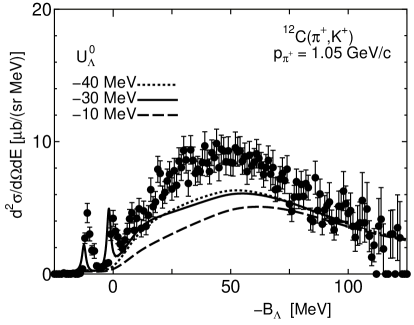
Figure 6: $(\pi^{+},K^{+})$ $\Lambda$ formation inclusive spectra with a ¹²C target at $\theta_{K}=6^{\circ}\mp 2^{\circ}$ for pions with $p_{\pi}=1.05$ GeV/$c$. These results were obtained with three choices of $U_{\Lambda}^{0}$ in a Woods-Saxon potential form with the geometry parameters of $r_{0}=1.25\times(A-1)^{1/3}$ fm and $a=0.65$ fm. The KEK data SAHA2 are also displayed.

IV.2 $\Sigma$ formation

In Ref. MK , we assumed an isotropic angular dependence for the $\pi^{-}+p\rightarrow K^{+}+\Sigma^{-}$ elementary process in calculating $(\pi^{-},K^{+})$ $\Sigma^{-}$ formation inclusive spectra. The energy dependence of $\sigma(\sqrt{s})$ was taken from the parameterization by Tsushima et al. THF , which was renormalized by a factor of 0.82. In this paper, we take into account the angular distribution using the Legendre polynomial coefficients reported by Good and Kofler GK on the basis of available data GK ; GOU ; DAHL ; DOY . Up to $\sqrt{s}\sim 2.1$ GeV, $p_{\pi}\sim 1900$ MeV/c, we can set $a_{\ell}=0$ with $\ell\geq 3$. We try to simulate the energy dependence of $a_{1}(\sqrt{s})$ and $a_{2}(\sqrt{s})$ by several lines as given in Table II, which are depicted in Fig.7 with the experimental data. The energy dependence of the total cross section $\sigma(\sqrt{s})$ is parameterized as follows:

$$\sigma(\sqrt{s}) = \frac{0.02055(\sqrt{s}-1.691)^{0.9603}}{(\sqrt{s}-1.682)^{2}+0.003131}$$ (26)

$$+ \frac{0.003023(\sqrt{s}-1.691)^{0.1394}}{(\sqrt{s}-1.894)^{2}+0.01548}\hskip 5.0pt\mbox{[mb]},$$

which is displayed by the solid curve in Fig. 8. At $\sqrt{s}=1.79$ GeV, corresponding to $p_{\pi}=1.2$ GeV/c, the absolute magnitude of the differential cross section at forward angles in the laboratory frame is about 130 $\mu$b, which corresponds well to that measured at KEK KEK .

Table 2: Legendre coefficients $a_{\ell}(\sqrt{s})$ in Eq. (17) of the differential cross sections of the $\pi^{-}+p\rightarrow K^{+}+\Sigma^{-}$ reaction, determined using experimental data GK ; GOU ; DAHL ; DOY .

	$a_{\ell}$		range of $\sqrt{s}$ (GeV)
$\ell=1$	$0.0$		$\sqrt{s}\leq 1.72$
	$-7.134(\sqrt{s}-1.72)$		$1.72<\sqrt{s}\leq 1.93$
	$-1.5$		$1.93<\sqrt{s}\leq 1.97$
	$6.25\sqrt{s}-13.81$		$1.97<\sqrt{s}\leq 2.05$
	$-1.0$		$2.05<\sqrt{s}\leq 2.15$
	$-4.06\sqrt{s}+7.729$		$2.15<\sqrt{s}\leq 2.31$
	$-1.65$		$2.31<\sqrt{s}$
$\ell=2$	$0.55$		$\sqrt{s}\leq 1.81$
	$8.0\sqrt{s}-13.93$		$1.81<\sqrt{s}\leq 1.89$
	$-7.44\sqrt{s}+15.25$		$1.89<\sqrt{s}\leq 2.05$
	$0.0$		$2.05<\sqrt{s}\leq 2.15$
	$10.0\sqrt{s}-21.5$		$2.15<\sqrt{s}\leq 2.31$
	$1.6$		$2.31<\sqrt{s}$

Figure 7: $\sqrt{s}$-dependence of Legendre coefficients of angular distributions of the $\pi^{-}+p\rightarrow K^{+}+\Sigma^{-}$ reaction. Empirical data points are taken from Refs. GK ; GOU ; DAHL ; DOY . The dotted and dashed lines show the fit for the calculation of $(\pi^{-},K^{+})$ inclusive spectra.

Figure 8: Total $\pi^{-}+p\rightarrow K^{+}+\Sigma^{-}$ cross sections as a function of the c.m. energy. Data points are taken from Refs. GK ; GOU ; DAHL ; DOY . The solid curve displays the parameterization of Eq. (23) in the present calculation. For comparison, the energy dependence used in Ref. MK with an isotropic angular dependence is shown by the dotted curve.

Figure 9: $(\pi^{-},K^{+})$ $\Sigma$ formation inclusive spectra with a ²⁸Si target at $\theta_{K}=6^{\circ}\mp 2^{\circ}$ for pions with $p_{\pi}=1.2$ GeV/$c$. These results were obtained with four choices of the repulsive strength $U_{\Sigma}^{0}=-10,10,30,50$ in a Woods-Saxon potential form with the geometry parameters of $r_{0}=1.25\times(A-1)^{1/3}$ fm and a=0.65 fm. Experimental data points are taken from Refs. KEK ; SAHA .

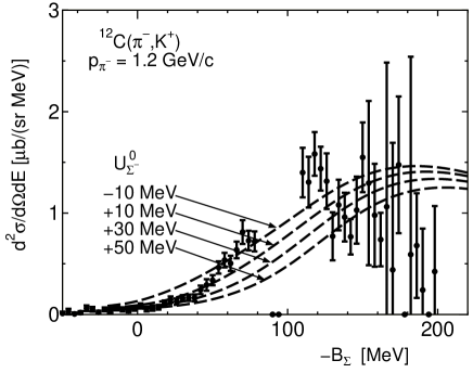
Figure 10: $(\pi^{-},K^{+})$ $\Sigma$ formation inclusive spectra with a ¹²C target at $\theta_{K}=6^{\circ}\mp 2^{\circ}$ for pions with $p_{\pi}=1.2$ GeV/$c$. These results were obtained with four choices of the repulsive strength $U_{\Sigma}^{0}=-10,10,30,50$ in a Woods-Saxon potential form with the geometry parameters of $r_{0}=1.25\times(A-1)^{1/3}$ fm and a=0.65 fm. Experimental data points are taken from Refs. SAHA .

Figures 9 and 10 compare calculated $(\pi^{-},K^{+})$ inclusive spectra with the KEK experimental data KEK ; SAHA . Several curves in these figures correspond to the assumed $\Sigma$ potential with $U_{\Sigma}^{0}=-10$, $10$, $30$ and $50$ MeV. In DWIA analyses in Refs. KEK ; SAHA and also in Ref. HH , an overall reduction factor is introduced to discuss the correspondence with the experimental data. However, we do not multiply any renormalization factor. It is seen that absolute values are satisfactorily reproduced by a repulsive strength of $10\sim 30$ MeV. Since we may expect additional contributions from multi-step processes, the actual repulsive strength may be larger than 30 MeV. This result agrees with that in Ref. MK , where the $\Sigma$ potential was concluded to be repulsive of the order of $30\sim 50$ MeV, using the SCDW model with the Thomas-Fermi approximation for the target nucleus, ²⁸Si. The assumption of the isotropic angular distribution of the elementary process used in Ref. MK tends to overestimate the elementary cross section at forward angles. Thus, the repulsive strength needed to reproduce the experimental data becomes smaller.

Table 3: Percentage contribution from each c.m. energy ($\sqrt{s}$) region of the $\pi^{-}+p\rightarrow K^{+}+\Sigma^{-}$ elementary process at $-B_{\Sigma}$ = 50, 110 and 170 MeV in $(\pi^{-},K^{+})$ $\Sigma$ formation inclusive spectra on ²⁸Si with $U_{\Sigma}^{0}=10$ and 30 MeV, respectively.

case of $U_{\Sigma}^{0}=10$ MeV
	$-B_{\Sigma}$ (MeV)
range of $\sqrt{s}$ (GeV)	50	110	170
$\sqrt{s}\leq 1.75$	0.0 %	0.0 %	3.7 %
1.75 $<\sqrt{s}\leq 1.80$	0.0 %	25.7 %	68.2 %
1.80 $<\sqrt{s}\leq 1.85$	21.8 %	62.7 %	27.3 %
1.85 $<\sqrt{s}\leq 1.90$	68.4 %	11.2 %	0.8 %
1.90 $<\sqrt{s}\leq 2.00$	9.7 %	0.4 %	0.0 %
2.00 $<\sqrt{s}$	0.1 %	0.0 %	0.0 %
case of $U_{\Sigma}^{0}=30$ MeV
	$-B_{\Sigma}$ (MeV)
range of $\sqrt{s}$ (GeV)	50	110	170
$\sqrt{s}\leq 1.75$	0.0 %	0.0 %	1.8 %
1.75 $<\sqrt{s}\leq 1.80$	0.0 %	18.1 %	48.3 %
1.80 $<\sqrt{s}\leq 1.85$	12.2 %	55.2 %	46.2 %
1.85 $<\sqrt{s}\leq 1.90$	66.6 %	25.0 %	3.6 %
1.90 $<\sqrt{s}\leq 2.00$	20.9 %	1.7 %	0.1 %
2.00 $<\sqrt{s}$	0.3 %	0.0 %	0.0 %

At present, the agreement of the calculated shape of the spectrum with the experimental data is not excellent. This may be related to the uncertainties of the input cross section, besides multi-step contributions. As is seen in Figs. 7 and 8, error bars of the elementary cross section are rather large. It is also to be born in mind that the $\Sigma$-nucleus potential may be energy-dependent. On the experimental side, the data is uncertain at the higher excitation energy region due to the spectrometer acceptance SAHA .

In order to learn the role of the nucleon Fermi motion, it is instructive to show which energy region of the elementary process dominantly contributes to the formation strength at each $\Sigma$ separation energy, $-B_{\Sigma}$. Table III tabulates percentage contributions from six different regions of $\sqrt{s}$ at $-B_{\Sigma}$ = 50, 110 and 170 MeV for the cases of $U_{\Sigma}^{0}=10$ and 30 MeV, respectively. At lower $\Sigma$ excitation energies, the reaction mainly occurs with a nucleon moving toward the incident pion. On the other hand, at higher $\Sigma$ energies, the dominant contribution comes from the elementary process at lower c.m. energies.

It was remarked in Ref. KEK that the peak position of the $(\pi^{-},K^{+})$ $\Sigma^{-}$ formation inclusive spectrum at an energy as high as 120 MeV is difficult to reproduce if the repulsion of the $\Sigma$-nucleus potential is not so strong as about 100 MeV. Our analysis suggests, however, that it is not necessary for the $\Sigma$ s.p. potential to be such repulsive. The reason that the result obtained in our SCDW model differs from that of Ref. KEK might be related to the fact that we did not use the factorization approximation represented by the average cross section, Eq. (2). The descriptions of incident pion and outgoing kaon distorted waves are also different. It will be worthwhile to detect the source of the different results.

It is necessary to discuss the correspondence of the $\Sigma$ potential strength obtained on the basis of the present $(\pi^{-},K^{+})$ inclusive spectra with the predictions of varying theoretical models for the $\Sigma N$ interaction. Most models NIJDF ; NIJNS of the Nijmegen group give an attractive $\Sigma$ s.p. potential, as is seen in various $G$-matrix calculations YB1 ; YB2 ; SCHU ; VIDA in nuclear matter. Only the model F is acceptable, which was concluded also by Da̧browski DAB in his plane wave impulse approximation analysis of the BNL data BNL of the $(K^{-},\pi^{+})$ spectrum on ⁹Be at $p_{K}=600$ MeV/c. The recent SU(6) quark model FU96a ; FU96b ; FU01 by Kyoto-Niigata group definitely predicts a repulsive $\Sigma$ s.p. potential. The $G$-matrix calculations KOH in symmetric nuclear matter showed that the early version, FSS FU96a ; FU96b , gives $U_{\Sigma}^{0}\sim+20$ MeV and the latest version, fss2 FU01 , $U_{\Sigma}^{0}\sim+8$ MeV. This repulsive $\Sigma$ s.p. potential originates from a strongly repulsive character in the isospin $T=\frac{3}{2}$ channel due to the quark anti-symmetrization effect. If the strength of more than 30 MeV is confirmed in future, these theoretical models will need fine tuning.

It is also important to pay attention to the density dependence of the $\Sigma$ s.p. potential. As the $\Sigma^{-}$ atomic data tells BFG , the $\Sigma$ potential is attractive at the very surface region of a nucleus. This feature is also seen in the $G$-matrix calculation with the quark model potential KOH . The calculation in this paper assumes a single Woods-Saxon form for the $\Sigma$ potential. A question whether the sign change of the $\Sigma^{-}$ potential can be detected or not at the outside region in the description of the $(\pi^{-},K^{+})$ reaction is to be studied in future. The energy dependence of the $\Sigma$ potential is another issue to be addressed. The $G$-matrix calculation in Ref. KOH indicates that the repulsive strength is not energy-independent.

Because of the strong repulsive contribution from the isospin $T=\frac{3}{2}$ channel, it is hypothesized that the $\Sigma^{-}$-nucleus potential becomes more repulsive in the case of a neutron excess. In this respect, analyses of the $(\pi^{-},K^{+})$ data with heavier nucleus targets will be interesting for the purpose of investigating whether such quantitative isospin dependence actually exists.

In the present calculations, there are various treatments to be improved. The smearing caused by the Lorentz-type convolution should be treated by the precise way of the Green’s function method, though much calculational efforts have to be devoted. A quantitative estimation of the contribution from multi-step processes is needed, which could fill the difference of the experimental data and the calculational results as is seen in the $\Lambda$ formation spectra. A model description of the elementary process is to be upgraded, though new experimental data is required to do it. After improving these points and the proper account of the CM motion of the target wave function, the SCDW framework serves as a quantitatively reliable model to study the possible modification of the elementary amplitudes in nuclear medium. The direction of the change of cross sections, increase or decrease, depends on how the amplitudes are altered through the underlying dynamical processes.

V Conclusions

We have developed a semiclassical distorted wave model for $(\pi,K)$ inclusive spectra corresponding to $\Lambda$ and $\Sigma$ formation processes, using the Wigner transformation of the nuclear density matrix. The expression of the double differential cross section consists of the incoming pion distorted wave function, the outgoing kaon distorted wave function and the undetected hyperon distorted wave function at each collision point, where the conservation of the classical local momenta is respected. The momentum distribution of the bound nucleon in the target nucleus is obtained from the Wigner transformation of Hartree-Fock wave functions.

We have first applied the model to inclusive $(\pi^{+},K^{+})$ $\Lambda$ formation spectra on the ²⁸Si and ¹²C targets measured at KEK SAHA . In this case, since the $\Lambda$ s.p. potential is well known, there is no adjustable parameter. The standard $\Lambda$ potential strength is found to reproduce well overall energy dependence of the data. The strength is underestimated. However, this is a rather preferable result, because the proper treatment of the CM motion has to be implemented in our SCDW formulation and there should be some contributions from two-step processes which are not taken into account. The quantitative estimation of these effects is one of the important subjects to be investigated.

Observing from the $(\pi^{+},K^{+})$ $\Lambda$ formation spectra that the SCDW model provides a useful description of the inclusive spectrum without any adjustable parameters and renormalization factors, we have proceeded to the $(\pi^{-},K^{+})$ $\Sigma$ formation spectra. The comparison of the calculated curves using several choices of the $\Sigma$ s.p. potential strength in a standard Woods-Saxon geometry with experimental data from KEK KEK ; SAHA has shown that an attractive $\Sigma$-nucleus potential overestimates the spectrum at lower excitation energies. Although there are rather large uncertainties in the information of the elementary process, we see that the repulsive potential is necessary to account for the absolute strength of the spectrum. Although we have to await quantitative estimation of various effects above mentioned to specify the strength of the $\Sigma$-nucleus potential, it is reasonable to conclude that the $\Sigma$ hyperon experiences repulsion in nuclear medium and its magnitude is not so strong as around 100 MeV which was suggested by DWIA analyses in Ref. KEK .

The information about the repulsive feature of the $\Sigma$-nucleus potential constrains the two-body $\Sigma$-$N$ potential model and thereby improves our understanding of the interactions between octet baryons. In the literature there has been a few $\Sigma$-$N$ potential models which predict repulsive $\Sigma$ mean field. In Nijmegen models NIJDF ; NIJNS , only the model F is satisfactory in this respect. Another model is a SU(6) quark model by the Kyoto-Niigata group FU96a ; FU96b ; FU01 . The model FSS gives 20 MeV KOH , on the other hand the more sophisticated version fss2 predicts somewhat smaller repulsion of 8 MeV. More studies are certainly needed to determine the strength of the $\Sigma$ s.p. potential, by employing various choice of the potential shapes. The energy dependence of the $\Sigma$-nucleus potential may also have to be taken into consideration.

The analyses of the data of heavier target nuclei are important in the next step. Since the neutron excess means that the $T=\frac{3}{2}$ contribution becomes larger, we could check the isospin dependence of the $\Sigma$-$N$ interaction on the basis of experimental data. The SCDW analyses of the data on ⁵⁸Ni, ¹¹⁵In and ²⁰⁹Bi taken at KEK SAHA are in progress.

Finally we note that the present framework can be straightforwardly extended to describe other inclusive spectra, such as $(K,\pi)$, $(K^{-},K^{+})$, $(\pi,\eta)$, $(\gamma,K)$, $(\gamma,\eta)$ and so on.

This study is supported by Grants-in-Aid for Scientific Research (C) from the Japan Society for the Promotion of Science (Grant Nos. 15540284, 15540270 and 17540263).

Appendix A Wigner transformation of the density matrix

We present an explicit expression for the Wigner transformation of the density matrix:

$$\Phi_{h}(\mbox{\boldmath$R$},\mbox{\boldmath$K$}) \equiv \frac{1}{(2\pi)^{3}}\int d\mbox{\boldmath$s$}\;e^{-i\mbox{\boldmath$s$}\cdot\mbox{\boldmath$K$}}$$ (27)

$$\times\sum_{h}\;\phi_{h}^{*}(\mbox{\boldmath$R$}-\frac{1}{2}\mbox{\boldmath$s$})\phi_{h}(\mbox{\boldmath$R$}+\frac{1}{2}\mbox{\boldmath$s$}).$$

We write the s.p. wave function of each partial wave in $r$-space as

$$\phi_{h}(\mbox{\boldmath$r$})=\frac{1}{r}\phi_{n_{h},\ell_{h},j_{h}}(r)[Y_{\ell_{h}}(\hat{\mbox{\boldmath$r$}})\times\chi_{1/2}]_{m_{h}}^{j_{h}},$$ (28)

where $\phi_{n_{h},\ell_{h},j_{h}}(r)$ is a radial wave function and $\chi_{1/2}$ a spin part. Let us denote the Fourier transform of the single-particle wave function $\phi_{h}(\mbox{\boldmath$r$})$ as $\tilde{\phi}_{h}(\mbox{\boldmath$k$})$.

$$\tilde{\phi}_{h}(\mbox{\boldmath$k$}) = \frac{1}{(2\pi)^{3}}\int d\mbox{\boldmath$r$}e^{-i\mbox{\boldmath$k$}\cdot\mbox{\boldmath$r$}}\phi_{h}(\mbox{\boldmath$r$})$$ (29)

$$= \frac{1}{(2\pi)^{\frac{3}{2}}}i^{2n_{h}-\ell_{h}}[Y_{\ell_{h}}(\hat{\mbox{\boldmath$k$}})\times\chi_{1/2}]_{m_{h}}^{j_{h}}$$

$$\times\frac{1}{k}\tilde{\phi}_{n_{h},\ell_{h},j_{h}}(k),$$

where $\hat{\mbox{\boldmath$k$}}$ represents angular parts of the vector $k$ and the Fourier transformation of the radial wave function is defined as

$$\frac{1}{k}\tilde{\phi}_{n_{h},\ell_{h},j_{h}}(k)=(-i)^{2n_{h}}\sqrt{\frac{2}{\pi}}\int dr\;rj_{\ell_{h}}(kr)\phi_{n_{h},\ell_{h},j_{h}}(r).$$ (30)

$\Phi_{h}(\mbox{\boldmath$R$},\mbox{\boldmath$K$})$ in Eq. (A1) is rewritten as

$$\Phi_{h}(\mbox{\boldmath$R$},\mbox{\boldmath$K$})=\int d\mbox{\boldmath$p$}\;\tilde{\phi}_{h}^{*}(\mbox{\boldmath$K$}-\frac{1}{2}\mbox{\boldmath$p$})\tilde{\phi}_{h}(\mbox{\boldmath$K$}+\frac{1}{2}\mbox{\boldmath$p$})\;e^{i\mbox{\boldmath$p$}\cdot\mbox{\boldmath$R$}}.$$ (31)

Using the expression of Eq. (A3), we first obtain

$$\sum_{m_{h}}\tilde{\phi}_{h}^{*}(\mbox{\boldmath$K$}-\frac{1}{2}\mbox{\boldmath$p$})\tilde{\phi}_{h}(\mbox{\boldmath$K$}+\frac{1}{2}\mbox{\boldmath$p$})$$ (32)

$$= \frac{1}{(2\pi)^{3}}\sum_{m_{h}}\;[Y_{\ell_{h}}(\widehat{\mbox{\boldmath$K$}-\frac{1}{2}\mbox{\boldmath$p$}})\times\chi_{1/2}]_{m_{h}}^{j_{h}*}$$

$$\times[Y_{\ell_{h}}(\widehat{\mbox{\boldmath$K$}+\frac{1}{2}\mbox{\boldmath$p$}})\times\chi_{1/2}]_{m_{h}}^{j_{h}}\frac{1}{|\mbox{\boldmath$K$}-\frac{1}{2}\mbox{\boldmath$p$}|}\frac{1}{|\mbox{\boldmath$K$}+\frac{1}{2}\mbox{\boldmath$p$}|}$$

$$\times\tilde{\phi}_{n_{h},\ell_{h},j_{h}}^{*}(|\mbox{\boldmath$K$}-\frac{1}{2}\mbox{\boldmath$p$}|)\tilde{\phi}_{n_{h},\ell_{h},j_{h}}(|\mbox{\boldmath$K$}+\frac{1}{2}\mbox{\boldmath$p$}|).$$

Since the spin part gives $\chi_{1/2\>m_{s}}^{*}\chi_{1/2\>m_{s}^{\prime}}\rightarrow\delta_{m_{s}m_{s}^{\prime}}$, the recoupling of angular momenta leads to the following expression.

$$\sum_{m_{h}}\tilde{\phi}_{h}^{*}(\mbox{\boldmath$K$}-\frac{1}{2}\mbox{\boldmath$p$})\tilde{\phi}_{h}(\mbox{\boldmath$K$}+\frac{1}{2}\mbox{\boldmath$p$})$$ (33)

$$= \frac{1}{(2\pi)^{3}}\frac{2j_{h}+1}{4\pi}P_{\ell_{h}}(\cos\theta_{\mbox{\boldmath$K$},\mbox{\boldmath$p$}})\frac{1}{|\mbox{\boldmath$K$}-\frac{1}{2}\mbox{\boldmath$p$}|}\frac{1}{|\mbox{\boldmath$K$}+\frac{1}{2}\mbox{\boldmath$p$}|}$$

$$\tilde{\phi}_{n_{h},\ell_{h},j_{h}}^{*}(|\mbox{\boldmath$K$}-\frac{1}{2}\mbox{\boldmath$p$}|)\tilde{\phi}_{n_{h},\ell_{h},j_{h}}(|\mbox{\boldmath$K$}+\frac{1}{2}\mbox{\boldmath$p$}|).$$

Here, the angle between $\mbox{\boldmath$K$}-\frac{1}{2}\mbox{\boldmath$p$}$ and $\mbox{\boldmath$K$}+\frac{1}{2}\mbox{\boldmath$p$}$ is denoted by $\theta_{\mbox{\boldmath$K$},\mbox{\boldmath$p$}}$; that is,

$$\cos\theta_{\mbox{\boldmath$K$},\mbox{\boldmath$p$}}=\frac{\mbox{\boldmath$K$}^{2}-\frac{1}{4}\mbox{\boldmath$p$}^{2}}{|\mbox{\boldmath$K$}-\frac{1}{2}\mbox{\boldmath$p$}||\mbox{\boldmath$K$}+\frac{1}{2}\mbox{\boldmath$p$}|}.$$ (34)

Then, Eq. (A5) becomes

$$\Phi_{h}(\mbox{\boldmath$R$},\mbox{\boldmath$K$}) = \int d\mbox{\boldmath$p$}\;e^{i\mbox{\boldmath$R$}\cdot\mbox{\boldmath$p$}}\;\frac{1}{(2\pi)^{3}}\frac{2j_{h}+1}{4\pi}$$

$$\times P_{\ell_{h}}(\cos\theta_{\mbox{\boldmath$K$},\mbox{\boldmath$p$}})\frac{1}{|\mbox{\boldmath$K$}-\frac{1}{2}\mbox{\boldmath$p$}|}\frac{1}{|\mbox{\boldmath$K$}+\frac{1}{2}\mbox{\boldmath$p$}|}$$

$$\times \tilde{\phi}_{n_{h},\ell_{h},j_{h}}^{*}(|\mbox{\boldmath$K$}-\frac{1}{2}\mbox{\boldmath$p$}|)\tilde{\phi}_{n_{h},\ell_{h},j_{h}}(|\mbox{\boldmath$K$}+\frac{1}{2}\mbox{\boldmath$p$}|).$$

Noting that the following relation holds

$$\int_{0}^{2\pi}d\phi_{p}\;e^{i\mbox{\boldmath$R$}\cdot\mbox{\boldmath$p$}} = 2\pi\sum i^{\ell}(2\ell+1)j_{\ell}(Rp)$$ (36)

$$\times P_{\ell}(\cos\widehat{\mbox{\boldmath$K$}\mbox{\boldmath$R$}})P_{\ell}(\cos\widehat{\mbox{\boldmath$K$}\mbox{\boldmath$p$}}),$$

we obtain the Legendre expansion of $\Phi_{h}(\mbox{\boldmath$R$},\mbox{\boldmath$K$})$. Each component $\Phi_{h}^{\ell}(R,K)$ of the expansion

$$\Phi_{h}(\mbox{\boldmath$R$},\mbox{\boldmath$K$})=\sum_{\ell=\mbox{even}}P_{\ell}(\cos\widehat{\mbox{\boldmath$K$}\mbox{\boldmath$R$}})\;\Phi_{h}^{\ell}(R,K)$$ (37)

is given as follows

$$\Phi_{h}^{\ell}(R,K) = 2\pi(-1)^{\ell/2}(2\ell+1)\int p^{2}dpd\cos\widehat{\mbox{\boldmath$K$}\mbox{\boldmath$p$}}\;j_{\ell}(Rp)P_{\ell}(\cos\widehat{\mbox{\boldmath$K$}\mbox{\boldmath$p$}})(2j_{h}+1)\frac{1}{(2\pi)^{3}}\frac{1}{4\pi}P_{\ell_{h}}(\cos\theta_{\mbox{\boldmath$K$},\mbox{\boldmath$p$}})$$ (38)

$$\times\frac{2}{\pi}\int dr\;rj_{\ell_{h}}(|\mbox{\boldmath$K$}+\frac{1}{2}\mbox{\boldmath$p$}|r)\phi_{n_{h},\ell_{h},j_{h}}(r)\int dr\;rj_{\ell_{h}}(|\mbox{\boldmath$K$}-\frac{1}{2}\mbox{\boldmath$p$}|r)\phi_{n_{h},\ell_{h},j_{h}}(r).$$

References

- (1) R. Bertini et al., Phys. Lett. B90, 375 (1980).
- (2) M. Kohno, R. Hausmann, P. Siegel and W. Weise, Nucl. Phys. A470, 609 (1987).
- (3) C. B. Dover, D. J. Millener and A. Gal, Phys. Rep. 184, 1 (1989).
- (4) R. S. Hayano et al., Phys. Lett. B231, 355 (1989).
- (5) T. Nagae et al., Phys. Rev. Lett. 80, 1605 (1998).
- (6) T. Harada, Phys. Rev. Lett. 81, 5287 (1998).
- (7) S. Bart et al., Phys. Rev. Lett. 83, 5238 (1999).
- (8) R. Sawafta, Nucl. Phys. A585, 103c (1995); A639, 103c (1998).
- (9) J. Da̧browski, Phys. Rev. C 60, 025205 (1999).
- (10) C. J. Batty, E. Friedman and A. Gal, Prog. Theor. Phys. Suppl. No. 117, 227 (1994).
- (11) M. M. Nagels, T. A. Rijken and J. J. de Swart, Phys. Rev. D 12, 744(1975); D 15 (1977), 2547; D 20, 1633 (1979).
- (12) Y. Yamamoto and H. Bando, Prog. Theor. Phys. 83, 254 (1990).
- (13) P. M. M. Maessen, T. A. Rijken and J. J. de Swart, Phys. Rev. C 40, 2226 (1989).
- (14) H.-J. Schulze, M. Baldo, U. Lombardo, J. Cugnon and A. Lejeune, Phys. Rev. C 57, 704 (1998).
- (15) Y. Fujiwara, C. Nakamoto and Y. Suzuki, Phys. Rev. Lett. 76, 2242 (1996).
- (16) Y. Fujiwara, C. Nakamoto and Y. Suzuki, Phys. Rev. C 54, 2180 (1996).
- (17) Y. Fujiwara, M. Kohno, C. Nakamoto and Y. Suzuki, Phys. Rev. C 64, 054001 (2001).
- (18) M. Kohno, Y. Fujiwara, T. Fujita, C. Nakamoto and Y. Suzuki, Nucl. Phys. A674, 229 (2000).
- (19) J. Mareš, E. Friedman, A. Gal and B.K. Jennings, Nucl. Phys. A594, 311 (1995).
- (20) J. Schaffner-Bielich and A. Gal, Phys. Rev. C 62, 034311 (2000).
- (21) N. Kaiser, Phys. Rev. C 71, 068201 (2005).
- (22) H. Noumi et al., Phys. Rev. Lett. 89 (2002), 072301; 90, 049902(E) (2003).
- (23) P.K. Saha et al., Phys. Rev. C 70, 044613 (2004).
- (24) T. Harada and Y. Hirabayashi, Nucl. Phys. A759, 143 (2005).
- (25) M. Kohno, Y. Fujiwara, K. Ogata, Y. Watanabe and M. Kawai, Prog. Thoer. Phys. 112, 895 (2004).
- (26) Y. L. Luo and M. Kawai, Phys. Lett. B235, 211 (1990); Phys. Rev. C 43, 2367 (1991).
- (27) Y. Watanabe et al., Phys. Rev. C 59, 2136 (1999).
- (28) K. Ogata, M. Kawai, Y. Watanabe, S. Weili and M. Kohno, Phys. Rev. C 60, 054605 (1999).
- (29) J.W. Negele and D. Vautherin, Phys. Rev. C 5, 1472 (1972).
- (30) Y. Horikawa, F. Lenz and N.C. Mukhopadhyay, Phys. Rev. C 22, 1680 (1980).
- (31) J.P. Elliot and T.H.R. Skyrme, Proc. Roy. Soc. A232, 561 (1955).
- (32) L.J. Tassie and F.C. Barker, Phys. Rev. 111, 940 (1958).
- (33) X. Campi and D. W. Sprung, Nucl. Phys. A194, 401 (1972).
- (34) G. Kahrimanis et al., Phys. Rev. C 55, 2533 (1997).
- (35) P.B. Siegel, W.B. Kaufmann and W.R. Gibbs, Phys. Rev. C 31, 2184 (1985).
- (36) D. Marlow et al., Phys. Rev. C 25, 2619 (1982).
- (37) R. Michael et al., Phys. Lett. B382, 29 (1996).
- (38) P.K. Saha, KEK Report 2001-17 (2001).
- (39) H. Bando, T. Motoba and J. Žofka, Int. J. Mod. Phys. 5, 4021 (1990).
- (40) R. D. Baker et al., Nucl. Phys. B141, 29 (1978).
- (41) D. H. Saxon et al., Nucl. Phys. B162, 522 (1980).
- (42) K. Tsushima, S. W. Huang and A. Faessler, Phys. Lett. B337, 245 (1994).
- (43) M.L. Good and R.R. Kofler, Phys. Rev. 183, 1142 (1969).
- (44) O. Goussu et al., Nuovo Cimento A42, 606 (1966).
- (45) O.I. Dahl, L.M. Hardy, R.I. Hess, J. Kirz, D.H. Miller and J.A. Schwartz, Phys. Rev. 163, 1142 (1967).
- (46) J.C. Doyle, F.S. Crawford and J.A. Anderson, Phys. Rev. 165, 1483 (1968).
- (47) Y. Yamamoto, T. Motoba, H. Himeno, K. Ikeda and S. Nagata, Prog. Theor. Phys. Suppl. No. 117, 361 (1994).
- (48) I. Vidaña, A. Polls, A. Ramos and H.-J. Schulze, Phys. Rev. C 64, 044301 (2001).