Multiplicity fluctuations
in relativistic nuclear collisions:
statistical model versus experimental data

Abstract

The multiplicity distributions of hadrons produced in central nucleus-nucleus collisions are studied within the hadron-resonance gas model in the large volume limit. The microscopic correlator method is used to enforce conservation of three charges – baryon number, electric charge, and strangeness – in the canonical ensemble. In addition, in the micro-canonical ensemble energy conservation is included. An analytical method is used to account for resonance decays. The multiplicity distributions and the scaled variances for negatively, positively, and all charged hadrons are calculated along the chemical freeze-out line of central Pb+Pb (Au+Au) collisions from SIS to LHC energies. Predictions obtained within different statistical ensembles are compared with the preliminary NA49 experimental results on central Pb+Pb collisions in the SPS energy range. The measured fluctuations are significantly narrower than the Poisson ones and clearly favor expectations for the micro-canonical ensemble. Thus this is a first observation of the recently predicted suppression of the multiplicity fluctuations in relativistic gases in the thermodynamical limit due to conservation laws.

I Introduction

For more than 50 years statistical models of strong interactions fermi ; landau ; hagedorn have served as an important tool to investigate high energy nuclear collisions. The main subject of the past study has been the mean multiplicity of produced hadrons (see e.g. Refs. stat1 ; FOC ; FOP ; pbm ). Only recently, due to a rapid development of experimental techniques, first measurements of fluctuations of particle multiplicity fluc-mult and transverse momenta fluc-pT were performed. The growing interest in the study of fluctuations in strong interactions (see e.g., reviews fluc1 ) is motivated by expectations of anomalies in the vicinity of the onset of deconfinement ood and in the case when the expanding system goes through the transition line between the quark-gluon plasma and the hadron gas fluc2 . In particular, a critical point of strongly interacting matter may be signaled by a characteristic power-law pattern in fluctuations fluc3 . Apart from being an important tool in an effort to study the critical behavior, the study of fluctuations in the statistical hadronization model constitutes a further test of its validity. In this paper we make, for the first time, predictions for the multiplicity fluctuations in central collisions of heavy nuclei calculated within the micro-canonical formulation of the hadron-resonance gas model. Fluctuations are quantified by the ratio of the variance of the multiplicity distribution and its mean value, the so-called scaled variance. The model calculations are compared with the corresponding preliminary results NA49 of NA49 on central Pb+Pb collisions at the CERN SPS energies.

There is a qualitative difference in the properties of the mean multiplicity and the scaled variance of multiplicity distribution in statistical models. In the case of the mean multiplicity results obtained with the grand canonical ensemble (GCE), canonical ensemble (CE), and micro-canonical ensemble (MCE) approach each other in the large volume limit. One refers here to the thermodynamical equivalence of the statistical ensembles. It was recently found CE ; res that corresponding results for the scaled variance are different in different ensembles, and thus the scaled variance is sensitive to conservation laws obeyed by a statistical system. The differences are preserved in the thermodynamic limit.

The paper is organized as follows. In Section II the microscopic correlators for a relativistic quantum gas are calculated in the MCE in the thermodynamical limit. This allows to take into account conservation of baryon number, electric charge, and strangeness in the CE formulation and, additionally, energy conservation in the MCE. In Section III the relevant formulas for the scaled variance of multiplicity fluctuations are presented for different statistical ensembles within the hadron-resonance gas model. The scaled variance of negative, positive and all charged hadrons is then calculated along the chemical freeze-out line in the temperature–baryon chemical potential plane. The fluctuations of hadron multiplicities in central Pb+Pb (Au+Au) collisions are presented for different collision energies from SIS to LHC. The results for the GCE, CE, and MCE are compared. In Section IV the statistical model predictions for the scaled variances and multiplicity distributions of negatively and positively charged hadrons are compared with the preliminary NA49 data of central Pb+Pb collisions in the SPS energy range. A summary, presented in Section V, closes the paper. New features of resonance decays within the MCE are discussed in Appendix A, and the acceptance procedure for all charged hadrons is considered in Appendix B.

II Multiplicity Fluctuations in Statistical Models

The mean multiplicities of positively, negatively and all charged particles are defined as:

$$\langle N_{-}\rangle\;=\;\sum_{i,q_{i}<0}\langle N_{i}\rangle\;,~{}~{}~{}~{}\langle N_{+}\rangle\;=\;\sum_{i,q_{i}>0}\langle N_{i}\rangle\;,~{}~{}~{}~{}\langle N_{ch}\rangle\;=\;\sum_{i,q_{i}\neq 0}\langle N_{i}\rangle\;,$$ (1)

where the average final state (after resonance decays) multiplicities $\langle N_{i}\rangle$ are equal to:

$$\langle N_{i}\rangle\;=\;\langle N_{i}^{*}\rangle+\sum_{R}\langle N_{R}\rangle\langle n_{i}\rangle_{R}\;.$$ (2)

In Eq. (2), $N_{i}^{*}$ denotes the number of stable primary hadrons of species $i$, the summation $\sum_{R}$ runs over all types of resonances $R$, and $\langle n_{i}\rangle_{R}\equiv\sum_{r}b_{r}^{R}n_{i,r}^{R}$  is the average over resonance decay channels. The parameters $b^{R}_{r}$ are the branching ratios of the $r$-th branches, $n_{i,r}^{R}$ is the number of particles of species $i$ produced in resonance $R$ decays via a decay mode $r$. The index $r$ runs over all decay channels of a resonance $R$, with the requirement $\sum_{r}b_{r}^{R}=1$. In the GCE formulation of the hadron-resonance gas model the mean number of stable primary particles, $\langle N_{i}^{*}\rangle$, and the mean number of resonances, $\langle N_{R}\rangle$, can be calculated as:

$$\langle N_{j}\rangle\;\equiv\;\sum_{\bf p}\langle n_{{\bf p},j}\rangle\;=\;\frac{g_{j}V}{2\pi^{2}}\int_{0}^{\infty}p^{2}dp\;\langle n_{{\bf p},j}\rangle\;,$$ (3)

where $V$ is the system volume and $g_{j}$ is the degeneracy factor of particle of the species $j$ (number of spin states). In the thermodynamic limit, $V\rightarrow\infty$, the sum over the momentum states can be substituted by a momentum integral. The $\langle n_{{\bf p},j}\rangle$ denotes the mean occupation number of a single quantum state labelled by the momentum vector ${\bf p}$ ,

$$\langle n_{{\bf p},j}\rangle~{} =~{}\frac{1}{\exp\left[\left(\epsilon_{{\bf p}j}-\mu_{j}\right)/T\right]~{}-~{}\alpha_{j}}~{},$$ (4)

where $T$ is the system temperature, $m_{j}$ is the mass of a particle $j$, $\epsilon_{{\bf p}j}=\sqrt{{\bf p}^{2}+m_{j}^{2}}$ is a single particle energy. A value of $\alpha_{j}$ depends on quantum statistics, it is $+1$ for bosons and $-1$ for fermions, while $\alpha_{j}=0$ gives the Boltzmann approximation. The chemical potential $\mu_{j}$ of a species $j$ equals to:

$$\mu_{j}~{}=~{}q_{j}~{}\mu_{Q}~{}+~{}b_{j}~{}\mu_{B}~{}+~{}s_{j}~{}\mu_{S}~{},$$ (5)

where $q_{j},~{}b_{j},~{}s_{j}$ are the particle electric charge, baryon number, and strangeness, respectively, while $\mu_{Q},~{}\mu_{B},~{}\mu_{S}$ are the corresponding chemical potentials which regulate the average values of these global conserved charges in the GCE. Eqs. (3-5) are valid in the GCE. In the limit $V\rightarrow\infty$ , Eq. (3-5) are also valid for the CE and MCE, if the energy density and conserved charge densities are the same in all three ensembles. This is usually referred to as the thermodynamical equivalence of all statistical ensembles. However, the thermodynamical equivalence does not apply to fluctuations.

In statistical models a natural measure of multiplicity fluctuations is the scaled variance of the multiplicity distribution. For negatively, positively, and all charged particles the scaled variances read:

$$\omega^{-}~{}=~{}\frac{\langle\left(\Delta N_{-}\right)^{2}\rangle}{\langle N_{-}\rangle}~{},~{}~{}~{}~{}\omega^{+}~{}=~{}\frac{\langle\left(\Delta N_{+}\right)^{2}\rangle}{\langle N_{+}\rangle}~{},~{}~{}~{}~{}\omega^{ch}~{}=~{}\frac{\langle\left(\Delta N_{ch}\right)^{2}\rangle}{\langle N_{ch}\rangle}~{}.$$ (6)

The variances in Eq. (6) can be presented as a sum of the correlators:

$$\langle\left(\Delta N_{-}\right)^{2}\rangle~{} =~{}\sum_{i,j;~{}q_{i}<0,q_{j}<0}\langle\Delta N_{i}\Delta N_{j}\rangle~{},~{}~{}~{}~{}\langle\left(\Delta N_{+}\right)^{2}\rangle~{}=~{}\sum_{i,j;~{}q_{i}>0,q_{j}>0}\langle\Delta N_{i}\Delta N_{j}\rangle~{},$$

$$\langle\left(\Delta N_{ch}\right)^{2}\rangle~{} =~{}\sum_{i,j;~{}q_{i}\neq 0,q_{j}\neq 0}\langle\Delta N_{i}\Delta N_{j}\rangle~{},$$ (7)

where $\Delta N_{i}\equiv N_{i}-\langle N_{i}\rangle$. The correlators in Eq. (7) include both the correlations between primordial hadrons and those of final state hadrons due to the resonance decays (resonance decays obey charge as well as energy-momentum conservation).

In the GCE the final state correlators can be calculated as Koch :

$$\langle\Delta N_{i}\,\Delta N_{j}\rangle_{g.c.e.}~{}=~{}\langle\Delta N_{i}^{*}\Delta N_{j}^{*}\rangle_{g.c.e.}\;+\;\sum_{R}\left[\langle\Delta N_{R}^{2}\rangle\;\langle n_{i}\rangle_{R}\;\langle n_{j}\rangle_{R}\;+\;\langle N_{R}\rangle\;\langle\Delta n_{i}\Delta n_{j}\rangle_{R}\right]~{},$$ (8)

where $\langle\Delta n_{i}~{}\Delta n_{j}\rangle_{R}\equiv\sum_{r}b_{r}^{R}n_{i,r}^{R}n_{j,r}^{R}~{}-~{}\langle n_{i}\rangle_{R}\langle n_{j}\rangle_{R}$ . The occupation numbers, $n_{{\bf p},j}$, of single quantum states (with fixed projection of particle spin) are equal to $n_{{\bf p},j}=0,1,\ldots,\infty$ for bosons and $n_{{\bf p},j}=0,1$ for fermions. Their average values are given by Eq. (4), and their fluctuations read:

$$\langle~{}\left(\Delta n_{{\bf p},j}\right)^{2}~{}\rangle~{}\equiv~{}\langle\left(n_{{\bf p},j}~{}-~{}\langle n_{{\bf p},j}\rangle\right)^{2}\rangle~{}=~{}\langle n_{{\bf p},j}\rangle\left(1~{}+~{}\alpha_{j}~{}\langle n_{{\bf p},j}\rangle\right)~{}\equiv~{}v^{2}_{{\bf p},j}~{}.$$ (9)

It is convenient to introduce a microscopic correlator, $\langle\Delta n_{{\bf p},j}\Delta n_{{\bf k},i}\rangle$, which in the GCE has a simple form:

$$\langle\Delta n_{{\bf p},j}~{}\Delta n_{{\bf k},i}\rangle_{g.c.e.}~{}=~{}\upsilon_{{\bf p},j}^{2}\,\delta_{ij}\,\delta_{{\bf p}{\bf k}}~{}.$$ (10)

Hence there are no correlations between different particle species, $i\neq j$, and/or between different momentum states, ${\bf p}\neq{\bf k}$. Only the Bose enhancement, $v_{{\bf p},j}^{2}>\langle n_{{\bf p},j}\rangle$ for $\alpha_{j}=1$, and the Fermi suppression, $v_{{\bf p},j}^{2}<\langle n_{{\bf p},j}\rangle$ for $\alpha_{j}=-1$, exist for fluctuations of primary particles in the GCE. The correlator in Eq. (8) can be presented in terms of microscopic correlators (10):

$$\langle\Delta N_{j}^{*}~{}\Delta N_{i}^{*}~{}\rangle_{g.c.e.}~{}=~{}\sum_{{\bf p},{\bf k}}~{}\langle\Delta n_{{\bf p},j}~{}\Delta n_{{\bf k},i}\rangle_{g.c.e.}~{}=~{}\delta_{ij}~{}\sum_{\bf p}~{}v_{{\bf p},j}^{2}~{}.$$ (11)

In the case of $i=j$ the above equation gives the scaled variance of primordial particles (before resonance decays) in the GCE.

In the MCE, the energy and conserved charges are fixed exactly for each microscopic state of the system. This leads to two modifications in a comparison with the GCE. First, the additional terms appear for the primordial microscopic correlators in the MCE. They reflect the (anti)correlations between different particles, $i\neq j$, and different momentum levels, ${\bf p}\neq{\bf k}$, due to charge and energy conservation in the MCE,

$$\langle\Delta n_{{\bf p},j}\Delta n_{{\bf k},i}\rangle_{m.c.e.}~{}=\;\upsilon_{{\bf p},j}^{2}\,\delta_{ij}\,\delta_{{\bf p}{\bf k}}\;-\;\frac{\upsilon_{{\bf p},j}^{2}v_{{\bf k},i}^{2}}{|A|}\;[\;q_{i}q_{j}M_{qq}+b_{i}b_{j}M_{bb}+s_{i}s_{j}M_{ss}$$

$$+~{}\left(q_{i}s_{j}+q_{j}s_{i}\right)M_{qs}~{}-~{}\left(q_{i}b_{j}+q_{j}b_{i}\right)M_{qb}~{}-~{}\left(b_{i}s_{j}+b_{j}s_{i}\right)M_{bs}$$

$$+~{}\epsilon_{{\bf p}j}\epsilon_{{\bf k}i}M_{\epsilon\epsilon}~{}-~{}\left(q_{i}\epsilon_{{\bf p}j}+q_{j}\epsilon_{{\bf k}i}\right)M_{q\epsilon}~{}+~{}\left(b_{i}\epsilon_{{\bf p}j}+b_{j}\epsilon_{{\bf k}i}\right)M_{b\epsilon}~{}-~{}\left(s_{i}\epsilon_{{\bf p}j}+s_{j}\epsilon_{{\bf k}i}\right)M_{s\epsilon}\;]\;,$$ (12)

where $|A|$ is the determinant and $M_{ij}$ are the minors of the following matrix,

$$A=\begin{pmatrix}\Delta(q^{2})&\Delta(bq)&\Delta(sq)&\Delta(\epsilon q)\\ \Delta(qb)&\Delta(b^{2})&\Delta(sb)&\Delta(\epsilon b)\\ \Delta(qs)&\Delta(bs)&\Delta(s^{2})&\Delta(\epsilon s)\\ \Delta(q\epsilon)&\Delta(b\epsilon)&\Delta(s\epsilon)&\Delta(\epsilon^{2})\end{pmatrix}\;,$$ (13)

with the elements, $\;\Delta(q^{2})\equiv\sum_{{\bf p},j}q_{j}^{2}\upsilon_{{\bf p},j}^{2}\;$, $\;\Delta(qb)\equiv\sum_{{\bf p},j}q_{j}b_{j}\upsilon_{{\bf p},j}^{2}\;$, $\;\Delta(q\epsilon)\equiv\sum_{{\bf p},j}q_{j}\epsilon_{{\bf p}j}\upsilon_{{\bf p},j}^{2}\;$, etc. The sum, $\sum_{{\bf p},j}$ , means integration over momentum ${\bf p}$, and the summation over all hadron-resonance species $j$ contained in the model. The first term in the r.h.s. of Eq. (II) corresponds to the microscopic correlator (10) in the GCE. Note that a presence of the terms containing a single particle energy, $\epsilon_{{\bf p}j}=\sqrt{{\bf p}^{2}+m_{j}^{2}}$, in Eq. (II) is a consequence of energy conservation. In the CE, only charges are conserved, thus the terms containing $\epsilon_{{\bf p}j}$ in Eq. (II) are absent. The $A$ in Eq. (13) becomes then the $3\times 3$ matrix (see Ref. res ). An important property of the microscopic correlator method is that the particle number fluctuations and the correlations in the MCE or CE, although being different from those in the GCE, are expressed by quantities calculated within the GCE. The microscopic correlator (II) can be used to calculate the primordial particle correlator in the MCE (or in the CE):

$$\langle\Delta N_{i}~{}\Delta N_{j}~{}\rangle_{m.c.e.} ~{}=\sum_{{\bf p},{\bf k}}~{}\langle\Delta n_{{\bf p},i}~{}\Delta n_{{\bf k},j}\rangle_{m.c.e.}\;.$$ (14)

A second feature of the MCE (or CE) is the modification of the resonance decay contribution to the fluctuations in comparison to the GCE (8). In the MCE it reads:

$$\langle\Delta N_{i}\,\Delta N_{j}\rangle_{m.c.e.}~{} =\;\langle\Delta N_{i}^{*}\Delta N_{j}^{*}\rangle_{m.c.e.}\;+\;\sum_{R}\langle N_{R}\rangle\;\langle\Delta n_{i}\;\Delta n_{j}\rangle_{R}\;+\;\sum_{R}\langle\Delta N_{i}^{*}\;\Delta N_{R}\rangle_{m.c.e.}\;\langle n_{j}\rangle_{R}\;$$

$$+\;\sum_{R}\langle\Delta N_{j}^{*}\;\Delta N_{R}\rangle_{m.c.e.}\;\langle n_{i}\rangle_{R}\;+\;\sum_{R,R^{\prime}}\langle\Delta N_{R}\;\Delta N_{R^{\prime}}\rangle_{m.c.e.}\;\langle n_{i}\rangle_{R}\;\langle n_{j}\rangle_{R^{{}^{\prime}}}\;.$$ (15)

Additional terms in Eq. (15) compared to Eq. (8) are due to the correlations (for primordial particles) induced by energy and charge conservations in the MCE. The Eq. (15) has the same form in the CE res and MCE, the difference between these two ensembles appears because of different microscopic correlators (II). The microscopic correlators of the MCE together with Eq. (14) should be used to calculate the correlators $\langle\Delta N_{i}^{*}\Delta N_{j}^{*}\rangle_{m.c.e.}$ , $\langle\Delta N_{i}^{*}\;\Delta N_{R}\rangle_{m.c.e.}~{}$, $~{}\langle\Delta N_{j}^{*}\;\Delta N_{R}\rangle_{m.c.e.}~{}$, $~{}\langle\Delta N_{R}\;\Delta N_{R^{\prime}}\rangle_{m.c.e.}$ entering in Eq. (15) .

The microscopic correlators and the scaled variance are connected with the width of the multiplicity distribution. It can be shown CLT that in statistical models the form of the multiplicity distribution derived within any ensemble (e.g. GCE, CE and MCE) approaches the Gauss distribution:

$$P_{G}(N)=\frac{1}{\sqrt{2\pi~{}\omega~{}\langle N\rangle}}~{}\exp\left[-\frac{\left(N~{}-~{}\langle N\rangle\right)^{2}}{2~{}\omega~{}\langle N\rangle}\right]~{}$$ (16)

in the large volume limit i.e. $\langle N\rangle\rightarrow\infty$. The width of this Gaussian, $\sigma=\sqrt{\omega~{}\langle N\rangle}$, is determined by the choice of the statistical ensemble, while from the thermodynamic equivalence of the statistical ensembles it follows that the expectation value $\langle N\rangle$ remains the same.

III multiplicity fluctuations at chemical freeze-out

In this section we present the results of the hadron-resonance gas for the scaled variances in the GCE, CE and MCE along the chemical freeze-out line in central Pb+Pb (Au+Au) collisions for the whole energy range from SIS to LHC. Mean hadron multiplicities in heavy ion collisions at high energies can be approximately fitted by the GCE hadron-resonance gas model. The fit parameters are the volume $V$, temperature $T$, chemical potential $\mu_{B}$, and the strangeness saturation parameter $\gamma_{S}$. The latter allows for non-equilibrium strange hadron yields. A recent discussion of system size and energy dependence of freeze-out parameters and comparison of freeze-out criteria can be found in Refs. FOP ; FOC . There are several programs designed for the analysis of particle multiplicities in relativistic heavy-ion collisions within the hadron-resonance gas model, see e.g., SHARE Share , THERMUS Thermus , and THERMINATOR Therminator . The set of model parameters, $V,T,\mu_{B}$, and $\gamma_{S}$, corresponds to the chemical freeze-out conditions in heavy-ion collisions. The numerical values and evolution of the model parameters with the collision energy are taken from previous analysis of multiplicities data. The dependence of $\mu_{B}$ on the collision energy is parameterized as FOC : $\mu_{B}\left(\sqrt{s_{NN}}\right)=1.308~{}\mbox{GeV}\cdot(1+0.273~{}\sqrt{s_{NN}})^{-1}~{},$ where the c.m. nucleon-nucleon collision energy, $\sqrt{s_{NN}}$, is taken in GeV units. The system is assumed to be net strangeness free, $S=0$, and to have the charge to baryon ratio of the initial colliding nuclei, $Q/B=0.4$. These two conditions define the system strange, $\mu_{S}$, and electric, $\mu_{Q}$, chemical potentials. For the chemical freeze-out condition we chose the average energy per particle, $\langle E\rangle/\langle N\rangle=1~{}$GeV Cl-Red . Finally, the strangeness saturation factor, $\gamma_{S}$, is parametrized FOP , $\gamma_{S}~{}=~{}1-0.396~{}\exp\left(-~{}1.23~{}T/\mu_{B}\right).$ This determines all parameters of the model. In this paper an extended version of THERMUS framework Thermus is used. A numerical procedure is applied to meet the above constraints simultaneously. Other choices of the freeze-out parameters will be discussed in the next section. The $T$, $\mu_{B}$, and $\gamma_{S}$ parameters used for different c.m. energies are given in Table I. Here, some further details should be mentioned. We use quantum statistics, but disregard the non-zero widths of resonances. The thermodynamic limit for the calculations of the scaled variance is assumed, thus $\omega$ reaches its limiting value, and volume $V$ is not a parameter of our model calculations. We also do not consider explicitly momentum conservation as it can be shown that it completely drops out in the thermodynamic limit CLT . Excluded volume corrections due to a hadron hard core volume are not taken into account. They will be considered elsewhere ExclVol . The standard THERMUS particle table includes all known particles and resonances up to a mass of about 2.5 GeV and their respective decay channels. Heavy resonances have not always well established decay channels. We re-scaled the branching ratios given in THERMUS to unity, where it was necessary to ensure a global charge conservation. Usually the resonance decays are considered in a successive manner, hence, each resonance decays into lighter ones until only stable particles are left. However, we need to implement another procedure when different branches are defined in a way that final states with only stable hadrons are counted. This distinction does not affect mean quantities, but for fluctuations it is crucial. To make a correspondence with NA49 data, both strong and electromagnetic decays should be taken into account, while weak decays should be omitted.

$\sqrt{s_{NN}}$	$T$	$\mu_{B}$	$\gamma_{S}$	$\;\omega^{-}\;$			$\;\omega^{+}\;$			$\;\omega^{ch}\;$
[ GeV ]	[ MeV ]	[ MeV ]		GCE	CE	MCE	GCE	CE	MCE	GCE	CE	MCE
$2.32$	64.9	800.8	0.641	1.025	0.777	0.578	1.020	0.116	0.086	1.048	0.403	0.300
$4.86$	118.5	562.2	0.694	1.058	0.619	0.368	1.196	0.324	0.192	1.361	0.850	0.505
$6.27$	130.7	482.4	0.716	1.069	0.640	0.346	1.203	0.390	0.211	1.431	0.969	0.524
$7.62$	138.3	424.6	0.735	1.078	0.664	0.334	1.200	0.442	0.222	1.476	1.060	0.534
$8.77$	142.9	385.4	0.749	1.084	0.683	0.328	1.197	0.479	0.230	1.504	1.126	0.541
$12.3$	151.5	300.1	0.787	1.097	0.729	0.320	1.185	0.563	0.247	1.557	1.271	0.558
$17.3$	157.0	228.6	0.830	1.108	0.768	0.318	1.174	0.637	0.263	1.593	1.393	0.576
$62.4$	163.1	72.7	0.975	1.127	0.827	0.316	1.147	0.782	0.298	1.636	1.609	0.613
$130$	163.6	36.1	0.998	1.131	0.827	0.313	1.141	0.805	0.305	1.639	1.631	0.618
$200$	163.7	23.4	1.000	1.133	0.826	0.312	1.140	0.811	0.307	1.639	1.636	0.619
$5500$	163.8	0.9	1.000	1.136	0.820	0.310	1.137	0.820	0.309	1.640	1.640	0.619

Table 1: The chemical freeze-out parameters $T$, $\mu_{B}$, $\gamma_{S}$, and final state scaled variances in the GCE, CE, and MCE for central Pb+Pb (Au+Au) collisions at different c.m. energies, $\sqrt{s_{NN}}$.

Once a suitable set of thermodynamical parameters is determined for each collision energy, the scaled variance of negatively, positively, and all charged particles can be calculated using Eqs. (6-7). The Eqs. (8-11) lead to the scaled variance in the GCE, whereas Eqs. (II-15) correspond to the MCE (or CE) results. The $\omega^{-},~{}\omega^{+},~{}\omega^{ch}$ in different ensembles are presented in Table I for different collision energies. The values of $\sqrt{s_{NN}}$ quoted in Table I correspond to the beam energies at SIS (2$A$ GeV), AGS (11.6$A$ GeV), SPS ($20A$, $30A$, $40A$, $80A$, and $158A$ GeV), colliding energies at RHIC ($\sqrt{s_{NN}}=62.4$ GeV, $130$ GeV, and $200$ GeV), and LHC ($\sqrt{s_{NN}}=5500$ GeV).

The mean multiplicities, $\langle N_{i}\rangle$, used for calculation of the scaled variance (see Eq. (6)) are given by Eqs. (2) and (3) and remain the same in all three ensembles. The variances in Eq. (6) are calculated using the corresponding correlators $\langle\Delta N_{i}\Delta N_{j}\rangle$ in the GCE, CE, and MCE. For the calculations of final state correlators the summation in Eq. (15) should include all resonances $R$ and $R^{\prime}$ which have particles of the species $i$ and/or $j$ in their decay channels. The resulting scaled variances are presented in Table I and shown in Figs. 1-3 as the functions of $\sqrt{s_{NN}}$.

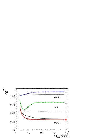
Figure 1: The scaled variances for negatively charged particles, $\omega^{-}$, both primordial and final, along the chemical freeze-out line for central Pb+Pb (Au+Au) collisions. Different lines present the GCE, CE, and MCE results. Symbols at the lines for final particles correspond to the specific collision energies pointed out in Table I. The arrows show the effect of resonance decays.

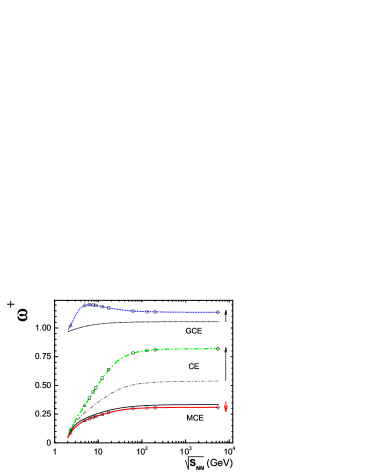
Figure 2: The same as in Fig. 1, but for $\omega^{+}$.

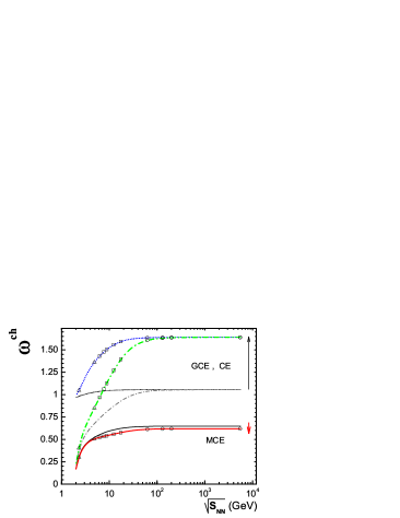
Figure 3: The same as in Figs. 1 and 2, but for $\omega^{ch}$.

At the chemical freeze-out of heavy-ion collisions, the Bose effect for pions and resonance decays are important and thus (see also Ref. res ): $\omega^{-}_{g.c.e.}\cong 1.1$, $\omega^{+}_{g.c.e.}\cong 1.2$, and $\omega^{ch}_{g.c.e.}\cong 1.4\div 1.6$, at the SPS energies. Note that in the Boltzmann approximation and neglecting the resonance decay effect one finds $\omega^{-}_{g.c.e.}=\omega^{+}_{g.c.e.}=\omega^{ch}_{g.c.e.}=1$.

Some qualitative features of the results should be mentioned. The effect of Bose and Fermi statistics is seen in primordial values in the GCE. At low temperatures most of charged hadrons are protons, and Fermi statistics dominates, $\omega^{+}_{g.c.e.},~{}\omega^{ch}_{g.c.e.}<1$. On the other hand, in the limit of high temperature (low $\mu_{B}/T$) most charged hadrons are pions and the effect of Bose statistics dominates, $\omega_{g.c.e.}^{\pm},~{}\omega_{g.c.e.}^{ch}>1$. Along the chemical freeze-out line, $\omega_{g.c.e.}^{-}$ is always slightly larger than 1, as $\pi^{-}$ mesons dominate at both low and high temperatures. The bump in $\omega^{+}_{g.c.e.}$ for final state particles seen in Fig. 2 at the small collision energies is due to a correlated production of proton and $\pi^{+}$ meson from $\Delta^{++}$ decays. This single resonance contribution dominates in $\omega^{+}_{g.c.e.}$ at small collision energies (small temperatures), but becomes relatively unimportant at the high collision energies.

A minimum in $\omega_{c.e.}^{-}$ for final particles is seen in Fig. 1. This is due to two effects. As the number of negatively charged particles is relatively small, $\langle N_{-}\rangle\ll\langle N_{+}\rangle$, at the low collision energies, both the CE suppression and the resonance decay effect are small. With increasing $\sqrt{s_{NN}}$, the CE effect alone leads to a decrease of $\omega^{-}_{c.e}$, but the resonance decay effect only leads to an increase of $\omega^{-}_{c.e}$. A combination of these two effects, the CE suppression and the resonance enhancement, leads to a minimum of $\omega^{-}_{c.e}$. As expected, $\omega_{m.c.e.}<\omega_{c.e.}$, as an energy conservation further suppresses the particle number fluctuations. A new feature of the MCE is the additional suppression of the fluctuations after resonance decays. This is discussed in Appendix A.

IV comparison with NA49 data

IV.1 Centrality Selection

The fluctuations in nucleus-nucleus collisions are studied on an event-by-event basis: a given quantity is measured for each collision and a distribution of this quantity is measured for a selected sample of these collisions. It has been found that the fluctuations in the number of nucleon participants give the dominant contribution to hadron multiplicity fluctuations. In the language of statistical models, fluctuations of the number of nucleon participants correspond to volume fluctuations caused by the variations in the collision geometry. Mean hadron multiplicities are proportional (in the large volume limit) to the volume, hence, volume fluctuations translate directly to the multiplicity fluctuations. Thus a comparison between data and predictions of statistical models should be performed for results which correspond to collisions with a fixed number of nucleon participants.

Due to experimental limitations it is only possible to approximately measure the number of participants of the projectile nucleus, $N_{P}^{proj}$, in fixed target experiments (e.g. NA49 at the CERN SPS). This is done in NA49 by measuring the energy deposited in a downstream Veto calorimeter. A large fraction of this energy is due to projectile spectators $N_{S}^{proj}$. Using baryon number conservation for the projectile nucleus ($A=N_{P}^{proj}+N_{S}^{proj}$) the number of projectile participants can be estimated. However, also a fraction of non-spectator particles, mostly protons and neutrons, contribute to the Veto energy NA49 . Furthermore, the total number of nucleons participating in the collision can fluctuate considerably even for collisions with a fixed number of projectile participants (see Ref. Voka ). This is due to fluctuations of the number of target participants. The consequences of the asymmetry in an event selection depend on the dynamics of nucleus-nucleus collisions (see Ref. MGMG for details). Still, for the most central Pb+Pb collisions selected by the number of projectile participants an increase of the scaled variance can be estimated to be smaller than a few % MGMG due to the target participant fluctuations. In the following our predictions will be compared with the preliminary NA49 data on the 1% most central Pb+Pb collisions at 20$A$-158$A$ GeV NA49 . The number of projectile participants for these collisions is estimated to be larger than 193.

IV.2 Modelling of Acceptance

In the experimental study of nuclear collisions at high energies only a fraction of all produced particles is registered. Thus, the multiplicity distribution of the measured particles is expected to be different from the distribution of all produced particles. Let us consider the production of $N$ particles with the probability $P_{4\pi}(N)$ in the full momentum space. If particle detection is uncorrelated, this means that the detection of one particle has no influence on the probability to detect another one, the binomial distribution can be used. For a fixed number of produced particles $N$ the multiplicity distribution of accepted particles reads:

$$P_{acc}(n,N)~{}=~{}q^{n}(1-q)^{N-n}~{}\cdot\frac{N!}{n!(N-n)!}~{},$$ (17)

where $n\leq N$ and $q$ is the probability of a single particle to be accepted (i.e. it is the ratio between mean multiplicity of accepted and all hadrons). Consequently one gets, $\overline{n}=q~{}N~{},~{}~{}\overline{n^{2}}-\overline{n}^{2}=q(1-q)N~{}$, where $\overline{n^{k}}\equiv\sum_{n=0}^{N}n^{k}P_{acc}(n,N)~{}$, for $k=1,2,\ldots$ . The probability distribution $P(n)$ of the accepted particles reads:

$$P(n)~{}=~{}\sum_{N=n}^{\infty}P_{4\pi}(N)~{}P_{acc}(n,N)~{}.$$ (18)

The first two moments of the distribution $P(n)$ are calculated as:

$$\langle n\rangle ~{}\equiv~{}\sum_{N=0}^{\infty}P_{4\pi}(N)~{}\sum_{n=0}^{N}n~{}P_{acc}(n,N)~{}=~{}q\cdot\langle N\rangle~{},$$ (19)

$$\langle n^{2}\rangle ~{}\equiv~{}\sum_{N=0}^{\infty}P_{4\pi}(N)~{}\sum_{n=0}^{N}n^{2}~{}P_{acc}(n,N)~{}=~{}q^{2}\cdot\langle N^{2}\rangle~{}+~{}q(1-q)\cdot\langle N\rangle~{},$$ (20)

where ($k=1,2,\ldots$)

$$\langle N^{k}\rangle~{}\equiv~{}\sum_{N=0}^{\infty}N^{k}~{}P_{4\pi}(N)~{}.$$ (21)

Finally, the scaled variance for the accepted particles can be obtained:

$$\omega~{}\equiv~{}\frac{\langle n^{2}\rangle~{}-~{}\langle n\rangle^{2}}{\langle n\rangle}~{}=~{}1~{}-~{}q~{}+q\cdot\omega_{4\pi}~{},$$ (22)

where $\omega_{4\pi}$ is the scaled variance of the $P_{4\pi}(N)$ distribution. The limiting behavior of $\omega$ agrees with the expectations. In the large acceptance limit ($q\approx 1$) the distribution of measured particles approaches the distribution in the full acceptance. For a very small acceptance ($q\approx 0$) the measured distribution approaches the Poisson one independent of the shape of the distribution in the full acceptance.

Model results on multiplicity fluctuations presented in Sec. III correspond to an ideal situation when all final hadrons are accepted by a detector. For a comparison with experimental data a limited detector acceptance should be taken into account. Even if primordial particles at chemical freeze-out are only weakly correlated in momentum space this would no longer be valid for final state particles as resonance decays lead to momentum correlations for final hadrons. In general, in statistical models, the correlations in momentum space are caused by resonance decays, quantum statistics and the energy-momentum conservation law, which is implied in the MCE. In this paper we neglect these correlations and use Eqs. (18) and (22). This may be approximately valid for $\omega^{+}$ and $\omega^{-}$, as most decay channels only contain one positively (or negatively) charged particle, but is certainly much worse for $\omega^{ch}$, for instance due to decays of neutral resonances into two charged particles. In order to limit correlations caused by resonance decays, we focus on the results for negatively and positively charged hadrons. A discussion of the effect of resonance decays to the acceptance procedure and a comparison with the data for $\omega^{ch}$ are presented in Appendix B. An improved modelling of the effect regarding the limited experimental acceptance will be a subject of a future study.

IV.3 Comparison with the NA49 Data for $\omega^{-}$ and $\omega^{+}$

Fig. 4 presents the scaled variances $\omega^{-}$ and $\omega^{+}$ calculated with Eq. (22).

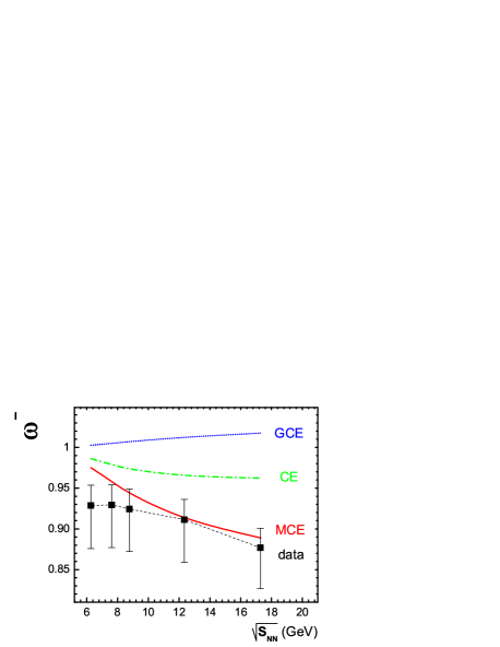
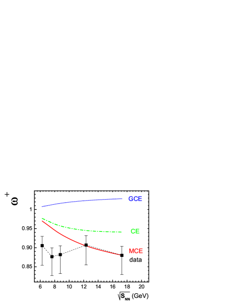
Figure 4: The scaled variances for negative (left) and positive (right) hadrons along the chemical freeze-out line for central Pb+Pb collisions at the SPS energies. The points show the preliminary data of NA49 NA49 . Total (statistical+systematic) errors are indicated. The statistical model parameters $T$, $\mu_{B}$, and $\gamma_{S}$ at different SPS collision energies are presented in Table I. Lines show the GCE, CE, and MCE results calculated with the NA49 experimental acceptance according to Eq. (22).

The hadron-resonance gas calculations in the GCE, CE, and MCE shown in Figs. 1 and 2 are used for the $\omega_{4\pi}^{\pm}$. The NA49 acceptance used for the fluctuation measurements is located in the forward hemisphere ($1<y(\pi)<y_{beam}$, where $y(\pi)$ is the hadron rapidity calculated assuming pion mass and shifted to the collision c.m. system NA49 ). The acceptance probabilities for positively and negatively charged hadrons are approximately equal, $q^{+}\approx q^{-}$, and the numerical values at different SPS energies are: $q^{\pm}=0.038,~{}0.063,~{}0.085,~{}0.131,~{}0.163$ at $\sqrt{s_{NN}}=6.27,~{}7.62,~{}8.77,~{}12.3,~{}17.3$ GeV, respectively. Eq. (22) has the following property: if $\omega_{4\pi}$ is smaller or larger than 1, the same inequality remains to be valid for $\omega$ at any value of $0<q\leq 1$. Thus one has a strong qualitative difference between the predictions of the statistical model valid for any freeze-out conditions and experimental acceptances. The CE and MCE correspond to $\omega_{m.c.e.}^{\pm}<\omega^{\pm}_{c.e.}<1$, and the GCE to $\omega_{g.c.e.}^{\pm}>1$.

From Fig. 4 it follows that the NA49 data for $\omega^{\pm}$ extracted from 1% of the most central Pb+Pb collisions at all SPS energies are best described by the results of the hadron-resonance gas model calculated within the MCE. The data reveal even stronger suppression of the particle number fluctuations.

IV.4 Dependence on the Freeze-out Parameters

The relation $E/N=1$ GeV Cl-Red was used in our calculations to define the freeze-out conditions. It does not give the best fit of the multiplicity data at each specific energy. In this subsection we check the dependence of the statistical model results for the scaled variances on the choice of the freeze-out parameters. For this purpose we compare the results obtained for the parameters used in this paper (model A) with two other sets of the freeze-out parameters at SPS energies: model B FOP and model C pbm . The corresponding values of $T$ and $\mu_{B}$ are presented in Fig. 5.

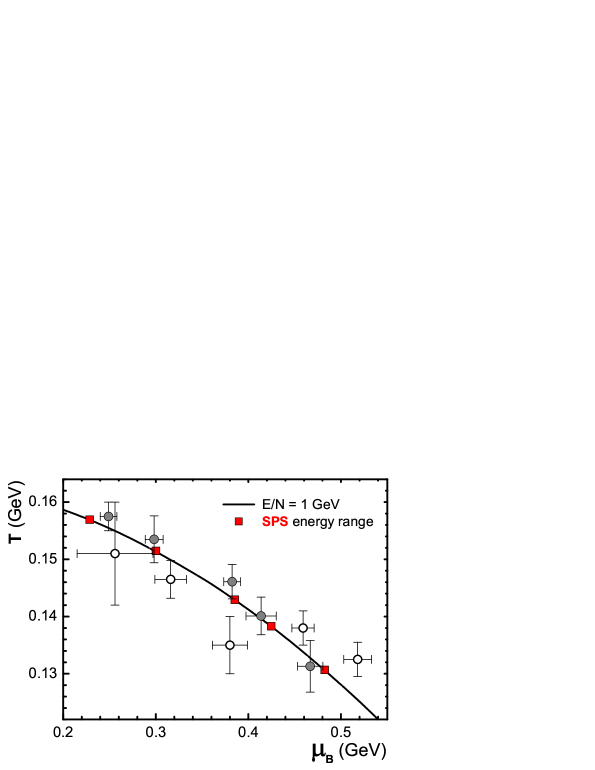
Figure 5: Chemical freeze-out points in the $T$-$\mu_{B}$ plane for central Pb+Pb collisions. The solid lines shows $\langle E\rangle/\langle N\rangle=1$ GeV, the squares are from our parametrization (model A) and denote SPS beam energies from $20A$ GeV (right) to $158A$ GeV (left), the full and open circles are the best fit parameters from reference FOP (model B) and pbm (model C), respectively.

$\sqrt{s_{NN}}$	$\;\omega_{m.c.e.}^{-}\;$			$\;\omega_{m.c.e.}^{+}\;$
[GeV]	A	B	C	A	B	C
$6.27$	0.346	0.345	0.361	0.211	0.214	0.210
$7.62$	0.334	0.334	0.347	0.222	0.225	0.221
$8.77$	0.328	0.330	0.330	0.230	0.232	0.236
$12.3$	0.320	0.318	0.325	0.247	0.249	0.248
$17.3$	0.318	0.317	0.321	0.263	0.264	0.259

Table 2: Final state scaled variances calculated in the MCE for 4 $\pi$ acceptance using freeze-out conditions A, B, and C.

The scaled variances $\omega_{m.c.e.}^{-}$ and $\omega_{m.c.e.}^{+}$ calculated in the full phase space within the MCE vary by less than 1% when changing the parameter set. In the NA49 acceptance the difference is almost completely washed out. The differences are somewhat stronger in the GCE and CE, but will not be considered here.

IV.5 Comparison of Distributions

As discussed in Section II the multiplicity distribution in statistical models in the full phase space and in the large volume limit approaches a normal distribution. If the particle detection is modelled by the simple procedure presented in Section IV B then the results (19-22) are valid for any form of the full acceptance distribution $P_{4\pi}(N)$. In the following we discuss the properties of the multiplicity distribution in the limited acceptance, $P(n)$, (18) and compare the statistical model results in different ensembles with data on negatively and positively charged hadrons.

For the Poisson distribution in the full acceptance the summation in Eq.(18) leads also to the Poisson distribution in the acceptance with the expectation value $\langle n\rangle=q\langle N\rangle$:

$$P(n)~{}=~{}\sum_{N=n}^{\infty}\frac{\langle N\rangle^{N}\exp[-\langle N\rangle]}{N!}~{}\cdot~{}\frac{q^{n}(1-q)^{N-n}~{}N!}{n!(N-n)!}~{}=~{}\exp[-q~{}\langle N\rangle]~{}\frac{\left(q~{}\langle N\rangle\right)^{n}}{n!}~{}.$$ (23)

However, the same does not hold true for summation in Eq. (18) being applied to other forms of the distribution $P(N)$. In particular, the normal distribution (16) is transformed into the following:

$$P(n)~{}=~{}\sum_{N=n}^{\infty}P_{G}(N)~{}P_{acc}(n,N)~{},$$ (24)

which is not anymore the Gauss one. It is enough to mention that a Gaussian is symmetric around its mean value, while the distribution (24) is not.

The average number particles accepted by a detector is:

$$\langle n\rangle~{}\equiv\sum_{n=0}^{\infty}n~{}P(n)~{}=~{}q~{}\langle N\rangle\equiv q~{}\rho~{}V~{},$$ (25)

where $\rho\equiv\langle N\rangle/V$ is the corresponding particle density. Hence, one can determine the volume to be

$$V~{}=~{}\frac{\langle N\rangle}{q~{}\rho}~{}.$$ (26)

In the following for each beam energy we adjust the volume to match the condition of Eq. (26) for negatively ($V^{-}$) and positively ($V^{+}$) charged yields, separately. Note that values for the volume are about $10-20$% larger than the ones in FOP ; pbm , which were obtained using a much less stringent centrality selection (here only the $1$% most central data is analyzed). We find that the $V^{-}$ and $V^{+}$ volume parameters deviate from each other by less than 10%. Deviations of a similar magnitude are observed between the data on hadron yield systematics and the hadron-resonance gas model fits. Here we are only interested in the shape of multiplicity distributions and do not attempt to optimize the model to fit simultaneously yields of positively and negatively charged particles. As typical examples the multiplicity distributions for negatively and positively charged hadrons produced in central Pb+Pb collisions at 40$A$ GeV are shown in Fig. 6 at the SPS energy range.

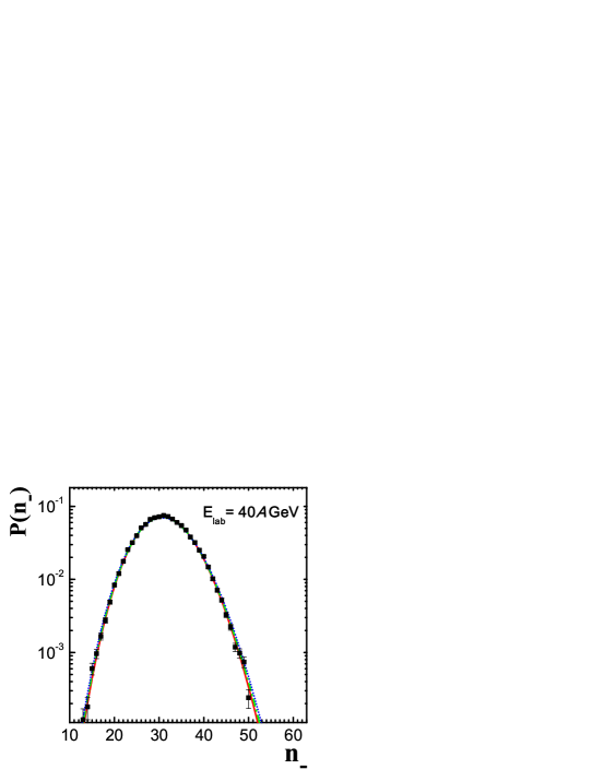
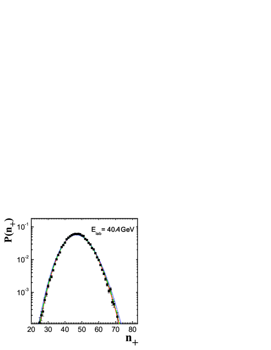
Figure 6: The multiplicity distributions for negatively (left) and positively (right) charged hadrons produced in central (1%) Pb+Pb collisions at 40$A$ GeV in the NA49 acceptance NA49 . The preliminary experimental data (solid points) of NA49 NA49 are compared with the prediction of the hadron-resonance gas model obtained within different statistical ensembles, the GCE (dotted lines), the CE (dashed-dotted lines) and the MCE (solid lines).

The bell-like shape of the measured spectra is well reproduced by the shape predicted by the statistical model. In the semi-logarithmic plot differences between the data and model lines obtained within different statistical ensembles are hardly visible. In order to allow for a detailed comparison of the distributions the ratio of the data and the model distributions to the Poisson one is presented in Fig. 7.

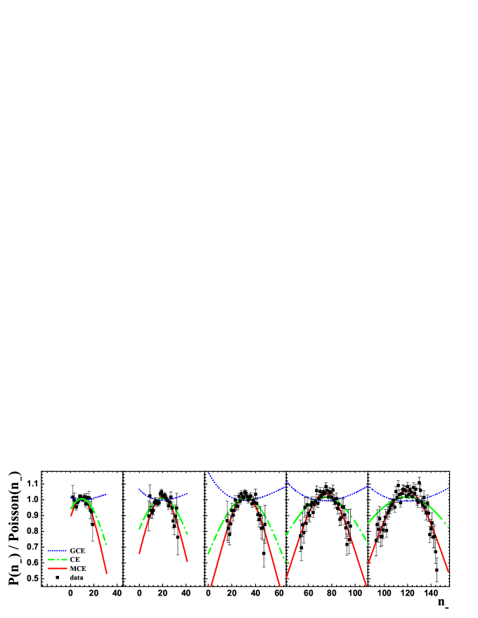
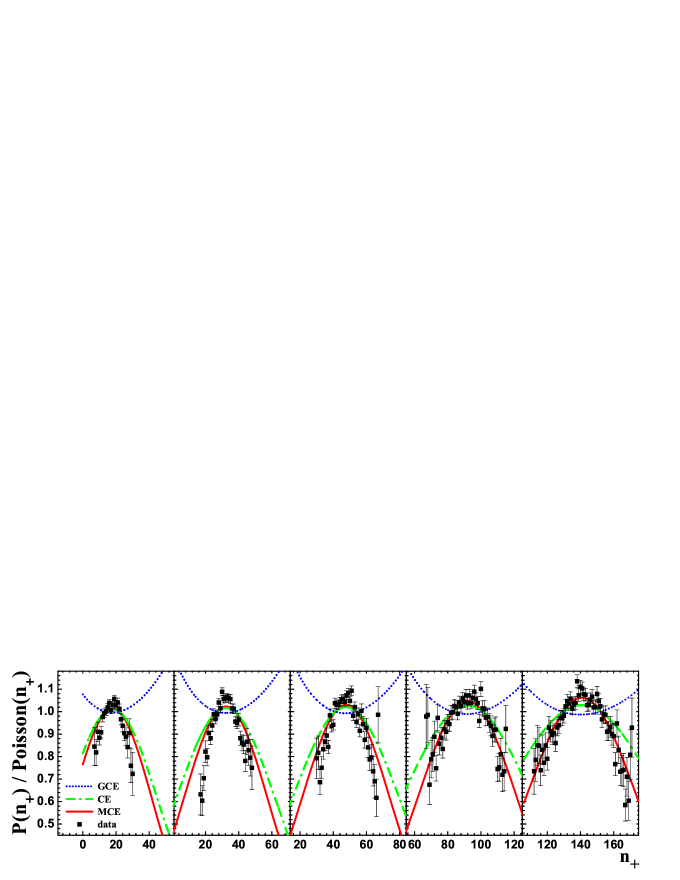
Figure 7: The ratio of the multiplicity distributions to Poisson ones for negatively (upper panel) and positively (lower panel) charged hadrons produced in central (1%) Pb+Pb collisions at 20$A$ GeV, 30$A$ GeV, 40$A$ GeV, 80$A$ GeV, and 158$A$ GeV (from left to right) in the NA49 acceptance NA49 . The preliminary experimental data (solid points) of NA49 NA49 are compared with the prediction of the hadron-resonance gas model obtained within different statistical ensembles, the GCE (dotted lines), the CE (dashed-dotted lines), and the MCE (solid lines).

The results for negatively and positively charged hadrons at 20$A$ GeV, 30$A$ GeV, 40$A$ GeV, 80$A$ GeV, and 158$A$ GeV are shown separately. The convex shape of the data reflects the fact that the measured distribution is significantly narrower than the Poisson one. This suppression of fluctuations is observed for both charges, at all five SPS energies and it is consistent with the results for the scaled variance shown and discussed previously. The GCE hadron-resonance gas results are broader than the corresponding Poisson distribution. The ratio has a concave shape. An introduction of the quantum number conservation laws (the CE results) leads to the convex shape and significantly improves agreement with the data. Further improvement of the agreement is obtained by the additional introduction of the energy conservation law (the MCE results). The measured spectra surprisingly well agree with the MCE predictions.

IV.6 Discussion

High resolution of the NA49 experimental data allows to distinguish between multiplicity fluctuations expected in hadron-resonance gas model for different statistical ensembles. The measured spectra clearly favor predictions of the micro-canonical ensemble. Much worse description is obtained for the canonical ensemble and a strong disagreement is seen considering the grand canonical one. All calculations are performed in the thermodynamical limit which is a proper approximation for the considered reactions. Thus these results should be treated as a first observation of the recently predicted CE suppression of multiplicity fluctuations due to conservation laws in relativistic gases in the large volume limit.

A validity of the micro-canonical description is surprising even within the framework of the statistical hadronization model used in this paper. This is because in the calculations the parameters of the model (e.g. energy, volume, temperature and chemical potential) were assumed to be the same in all collisions. On the other hand, significant event-by-event fluctuations of these parameters may be expected. For instance, only a part of the total energy is available for the hadronization process. This part should be used in the hadron-resonance gas calculations while the remaining energy is contained in the collective motion of matter. The ratio between the hadronization and collective energies may vary from collision to collision and consequently increase the multiplicity fluctuations.

The agreement between the data and the MCE predictions is even more surprising when the processes which are beyond the statistical hadronization model are considered. Examples of these are jet and mini-jet production, heavy cluster formation, effects related to the phase transition or instabilities of the quark-gluon plasma. Naively all of them are expected to increase multiplicity fluctuations and thus lead to a disagreement between the data and the MCE predictions. A comparison of the data with the models which include these processes is obviously needed for significant conclusions. Here we consider only one example.

In Ref. ood a non-monotonic dependence of the relative fluctuations,

$$R_{e}~{}=~{}\frac{(\delta S)^{2}/S^{2}}{(\delta E)^{2}/E^{2}}~{},$$ (27)

has been suggested as a signal for the onset of deconfinement. Here $S$ and $E$ denote the system entropy and thermalized energy at the early stage of collisions, respectively. This prediction assumes event-by-event fluctuations of the thermalized energy, which results in the fluctuations of the produced entropy. The ratio of the entropy to energy fluctuations (27) depends on the equation of state and thus on the form of created matter. The $R_{e}$ is approximately independent of collision energy and equals about $0.6$ in pure hadron or quark-gluon plasma phases. An increase of the $R_{e}$ ratio up to its maximum value, $R_{e}\approx 0.8$, is expected ood in the transition domain. Anomalies in energy dependence of the hadron production properties measured in central Pb+Pb collisions NA49-1 indicate mg2 that the transition domain is located at the low CERN SPS energies, from 30$A$ to 80$A$ GeV. Thus an anomaly in the energy dependence of multiplicity fluctuations is expected in the same energy domain ood .

In any case the fluctuations of the thermalized energy will lead to additional multiplicity fluctuations (“dynamical fluctuations”). The resulting contribution to the scaled variance can be calculated to be:

$$\omega^{-}_{dyn}~{}=~{}R_{e}~{}\langle n_{-}\rangle~{}\frac{(\delta E)^{2}}{E^{2}}~{}.$$ (28)

The above assumes that the mean particle multiplicity is proportional to the early stage entropy. In order to perform a quantitative estimate of the effect the fluctuations of the energy of produced particles were calculated within the HSD hsd and UrQMD urqmd string-hadronic models. For central (impact parameter zero) Pb+Pb collisions in the energy range from 30A to 80A GeV we have obtained, $\sqrt{(\delta E)^{2}}/E\leq 0.03$. The number of accepted negatively charged particles is $\langle n_{-}\rangle\approx 30$ at $40A$ GeV (see Fig. 7). Thus, an increase of the $\omega$ due to the “dynamical fluctuations” estimated by Eq. (28) is $\omega^{-}_{dyn}\leq 0.02$ for $R_{e}=0.6$, and it is smaller than the experimental error of the preliminary NA49 data of about 0.05 NA49 . In particular, an additional increase due to the phase transition, $\Delta\omega^{-}_{dyn}\approx 0.005$, for $R_{e}=0.8$, can be hardly observed.

In conclusion, the predicted ood increase of the scaled variance of the multiplicity distribution due to the onset of deconfinement is too small to be observed in the current data. These data neither confirm nor refute the interpretation mg2 of the measured NA49-1 anomalies in the energy depedence of other hadron production properties as due to the onset of deconfinement at the CERN SPS energies.

More differential data on multiplicity fluctuations and correlations are required for further tests of the validity of the statistical models and observation of possible signals of the phase transitions. The experimental resolution in a measurement of the enhanced fluctuations due to the onset of deconfinement can be increased by increasing acceptance. For example, $\omega_{dyn}^{-}\propto\langle n_{-}\rangle\propto q$. The present aceptance of NA49 at 40$A$ GeV is about $q\cong 0.06$ and it can be increased up to about $q\cong 0.5$ in the future studies. This will give a chance to observe, for example, the dynamical fluctuations discussed in Ref. ood . The observation of the MCE suppression effects of the multiplicity fluctuations by NA49 was possible only because a selection of a sample of collisions without projectile spectators. This selection seems to be possible only in the fixed target experiments. In the collider kinematics nuclear fragments which follow the beam direction can not be measured.

On the model side a further study is needed to improve description of the effect of the limited experimental acceptance. Further on, a finite volume of hadrons is expected to lead to a reduction of the particle number fluctuations ExclVol . A quantitative estimate of this effect is needed.

V Summary

The hadron multiplicity fluctuations in relativistic nucleus-nucleus collisions have been predicted in the statistical hadron-resonance gas model within the grand canonical, canonical, and micro-canonical ensembles in the thermodynamical limit. The microscopic correlator method has been extended to include three conserved charges – baryon number, electric charge, and strangeness – in the canonical ensemble, and additionally an energy conservation in the micro-canonical ensemble. The analytical formulas are used for the resonance decay contributions to the correlations and fluctuations. The scaled variances of negatively, positively, and all charged particles for primordial and final state hadrons have been calculated at the chemical freeze-out in central Pb+Pb (Au+Au) collisions for different collision energies from SIS to LHC. A comparison of the multiplicity distributions and the scaled variances with the preliminary NA49 data on Pb+Pb collisions at the SPS energies has been done for the samples of about 1% of most central collisions selected by the number of projectile participants. This selection allows to eliminate effect of fluctuations of the number of nucleon participants. The effect of the limited experimental acceptance was taken into account by use of the uncorrelated particle approximation.

The measured multiplicity distributions are significantly narrower than the Poisson one and allow to distinguish between model results derived within different statistical ensembles. The data surprisingly well agree with the expectations for the micro-canonical ensemble and exclude the canonical and grand-canonical ensembles. Thus this is a first experimental observation of the predicted suppression of the multiplicity fluctuations in relativistic gases in the thermodynamical limit due to conservation laws.

Appendix A Resonance decays in the MCE

A comparison of the primordial scaled variances with those for final hadrons demonstrates that the fluctuations generally increase after resonance decays in the GCE and CE (see more details in Ref. res ), but they decrease in the MCE. In order to understand this effect let us consider a toy model $(\pi^{+},\pi^{-},\rho^{0})$-system with a zero net charge, $Q=0$. Due to this last condition there is a full symmetry between positively and negatively charged pions, and thus $\omega^{+}=\omega^{-}$. Each $\rho^{0}$-meson decays into a $\pi^{+}\pi^{-}$-pair with 100% probability, i.e. $b_{1}^{\rho}=1$ and $\langle n_{-}\rangle_{\rho^{0}}=1$. The predictions of the CE and MCE for $(\pi^{+},\pi^{-},\rho^{0})$-system are shown in Fig. 8.

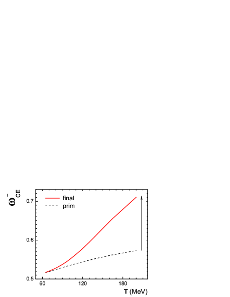
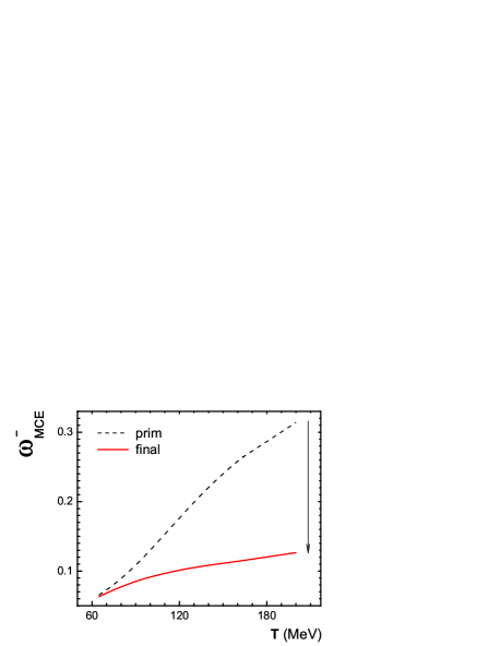
Figure 8: The scaled variance for negatively charged particles, $\omega^{-}$, in the toy $(\pi^{+},\pi^{-},\rho^{0})$-system with $Q=0$ in the CE (left) and MCE (right) as a function of temperature. The temperature interval corresponds to that presented in Table I. The dotted lines correspond to primordial $\pi^{-}$-meson fluctuations, the solid lines – to those after $\rho^{0}$ decays. At small $T$ the $\rho^{0}$ contribution to the pion number fluctuations is negligible, and it increases with $T$. The contribution from $\rho^{0}$ decays to $\omega^{-}$ is positive in the CE and negative in the MCE (see the text for details).

One observes that $\rho^{0}$ decays lead to an enhancement of $\omega^{-}$ in the CE, and to its suppression in the MCE. In the CE one finds from Eqs. (2) and (15) for $(\pi^{+},\pi^{-},\rho^{0})$-system:

$$\langle N_{-}\rangle~{}=~{}\langle N_{\pi^{-}}^{*}\rangle~{}+~{}\langle N_{\rho^{0}}\rangle\;,~{}~{}~{}~{}\langle\left(\Delta N_{-}\right)^{2}\rangle_{c.e.}~{}=~{}\langle\left(\Delta N_{\pi^{-}}^{*}\right)^{2}\rangle_{c.e.}~{}+~{}\langle\left(\Delta N_{\rho^{0}}\right)^{2}\rangle_{c.e.}\;.$$ (29)

Note that the average multiplicities, $\langle N_{\pi^{-}}^{*}\rangle$ and $\langle N_{\rho^{0}}\rangle$, remain the same in the CE, and the MCE. From Eq. (29) it follows:

$$\omega_{c.e.}^{-}~{}=~{}\omega_{c.e.}^{-*}~{}\left[\frac{\langle N_{\pi^{-}}^{*}\rangle~{}+~{}(\omega_{c.e.}^{\rho^{0}}/\omega_{c.e.}^{-*})\cdot\langle N_{\rho^{0}}\rangle}{\langle N_{-}\rangle}\right]~{}.$$ (30)

The $\omega_{c.e.}^{-*}$ is essentially smaller than 1 due to the strong CE suppression (see Fig. 8, left). On the other hand, there is no CE suppression for $\rho^{0}$ fluctuations, $\omega_{c.e.}^{\rho^{0}}=\omega_{g.c.e.}^{\rho^{0}}\cong 1$. Therefore, one finds that $\omega_{c.e.}^{\rho^{0}}/\omega_{c.e.}^{-*}>1$, and from Eq. (30) it immediately follows, $\omega_{c.e.}^{-}~{}>~{}\omega_{c.e.}^{-*}$. Note that $\omega_{g.c.e.}^{-*}\cong\omega_{g.c.e.}^{\rho^{0}}\cong 1$, thus there is no enhancement of $\omega_{g.c.e.}^{-}$ due to $\rho^{0}$ decays. In the MCE the multiplicity $\langle N_{-}\rangle$ remains the same as in Eq. (29). The variance $\langle\left(\Delta N_{-}\right)^{2}\rangle_{m.c.e.}$ is, however, modified because of the anti-correlation between primordial $\pi^{-*}$ and $\rho^{0}$ mesons in the MCE. From Eq. (15) one finds for our $(\pi^{+},\pi^{-},\rho^{0})$-system,

$$\langle\left(\Delta N_{-}\right)^{2}\rangle_{m.c.e.}~{}=~{}\langle\left(\Delta N_{\pi^{-}}^{*}\right)^{2}\rangle_{m.c.e.}~{}+~{}\langle\left(\Delta N_{\rho^{0}}\right)^{2}\rangle_{m.c.e.}~{}+~{}2~{}\langle\Delta N_{\pi^{-}}^{*}~{}\Delta N_{\rho^{0}}\rangle_{m.c.e.}~{}.$$ (31)

The last term in Eq. (31) appears due to energy conservation in the MCE (it is absent in the CE). This term is evidently negative, which means that an anti-correlation occurs. A large (small) number of primordial pions, $\Delta N_{\pi^{-}}^{*}>0~{}(<0)$, requires a small (large) number of $\rho^{0}$-mesons, $\Delta N_{\rho^{0}}<0~{}(>0)$, to keep the total energy fixed. Anti-correlation between primordial pions and $\rho^{0}$-mesons makes the $\pi^{-}$ number fluctuations smaller after resonance decays, i.e. $\omega_{m.c.e.}^{-}<\omega_{m.c.e.}^{-*}$, as depicted in Fig. 8 (right). The same mechanism works in the MCE for the full hadron-resonance gas.

Appendix B Acceptance effect for All Charged Particles

In order to better understand an influence of the momentum correlation due to resonance decays on the multiplicity fluctuations we define a toy model. Let us assume that there are two kinds of particles produced. The first kind ($N$) is either stable or originates from decay channels which contain only one particle of the type we are set to investigate, while the second kind ($M$) produces 2 particles of the selected type. This is described by the (unknown) probability distribution $P_{4\pi}\left(N,M\right)$. We further assume that for both types of particles, $N$ and $M$, separately the acceptance procedure defined by Eq. (17) is applicable. We also assume that once particle $M$ is inside the experimental acceptance, both its decay products will be so as well. Hence, the average number of observed particles will be:

$$\langle n\rangle~{}=~{}\sum_{N=0}^{\infty}\sum_{M=0}^{\infty}~{}P_{4\pi}\left(N,M\right)~{}\sum_{n=0}^{N}\sum_{m=0}^{M}~{}(n+2~{}m)~{}P_{acc}\left(n,N\right)P_{acc}\left(m,M\right)~{}.$$ (32)

This leads immediately to:

$$\langle n\rangle~{}=~{}q\cdot\Big{[}\langle N\rangle+2~{}\langle M\rangle\Big{]}~{}.$$ (33)

One finds the second moment,

$$\langle n^{2}\rangle~{}=~{}\sum_{N=0}^{\infty}\sum_{M=0}^{\infty}~{}P_{4\pi}\left(N,M\right)~{}\sum_{n=0}^{N}\sum_{m=0}^{M}~{}(n+2m)^{2}~{}P_{acc}\left(n,N\right)P_{acc}\left(m,M\right)~{}.$$ (34)

Making use of the relation (20) one obtains:

$$\langle n^{2}\rangle~{}=~{}q\left(1-q\right)\cdot\langle N\rangle~{}+~{}q^{2}\cdot\langle N^{2}\rangle~{}+~{}4q^{2}\cdot\langle NM\rangle~{}+~{}4q\left(1-q\right)\cdot\langle M\rangle~{}+~{}4q^{2}\cdot\langle M^{2}\rangle~{}.$$ (35)

Thus, for the scaled variance it follows:

$$\omega~{}\equiv~{}\frac{\langle n^{2}\rangle-\langle n\rangle^{2}}{\langle n\rangle}~{}=~{}q\cdot\omega_{4\pi}~{}+~{}\left(1-q\right)\cdot\Bigg{[}\frac{\langle N\rangle+4~{}\langle M\rangle}{\langle N\rangle+2~{}\langle M\rangle}\Bigg{]}~{},$$ (36)

where $\omega_{4\pi}$ is obtained from the case $q=1$ and corresponds to the original distribution $P_{4\pi}\left(N,M\right)$. For the second limiting case of Eq. (36), $q\rightarrow 0$, one finds a scaled variance which corresponds to that of two uncorrelated Poisson distributions with means $q\langle N\rangle$ and $q\langle M\rangle$, respectively. In this case, all primordial correlations due to energy and charge conservation or Bose (Fermi) statistics are lost, but particles produced by resonances of type $M$ are still detected in pairs.

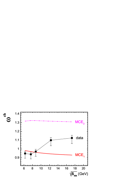
Figure 9: Left. Fraction of total yield originating from resonance decays with 2 or more positively(‘+’), negatively(‘-’), or all charged(‘ch’), particles. Parameters are taken from parametrization in section III. Right. The scaled variances for all charged hadrons along the chemical freeze-out line for central Pb+Pb collisions at the SPS energies. The points show the preliminary data of NA49. The statistical model parameters $T$, $\mu_{B}$, and $\gamma_{S}$ at different SPS collision energies are presented in Table I. The lines show the MCE results calculated with the NA49 experimental acceptance according to Eq. (22) (lower line) and Eq. (38) ( upper line).

In general case, by $k$ we denote the fraction of particles originating from decays (always 2 relevant daughters) of particle kind $M$, hence,

$$\langle N\rangle~{}=~{}\left(1-k\right)~{}\langle N_{tot}\rangle~{},\qquad\langle M\rangle~{}=~{}\frac{k}{2}~{}\langle N_{tot}\rangle~{}.$$ (37)

Finally, one finds for the scaled variance:

$$\omega~{}=~{}q\cdot\omega_{4\pi}~{}+~{}\left(1-q\right)\left(1+k\right)~{}.$$ (38)

From the hadron-resonance gas model we can estimate the fraction $k$ of the final yield which originates from decays of resonances into 2 (or more) charged particles. From Fig. 9 (left) we find the fraction of the charged particle yield $k$ to be from 35% ($20$ AGeV) to 45% ($158$ AGeV) in the SPS energy range (and about 10% for positively and negatively charged particles). For the definition of decay channels see section III. Examples of two-particle decay channels: $\rho^{0}\rightarrow\pi^{+}+\pi^{-}$, would be counted as two particle decay in ‘ch’, but neither in ‘+’ nor in ‘-’, $\Delta^{++}\rightarrow p+\pi^{+}$, would contribute to ‘ch’ and ‘+’, but not to ‘-‘. The assumption that both decay products are detected is certainly not justifiable for small values of the total acceptance $q$, hence Eq. (38) overestimates the effect. However, this consideration will give a useful upper bound (see Fig. 9, right). The typical width of decays is comparable to the width of the acceptance window, therefore, about half of all decays will leave one (or both) decay product missing. Yet the same 50% will be contributed from decays whose parents are outside the acceptance but contribute to the final yield. Hence, one expects no change in average multiplicity, but a sizable effect on fluctuations.

References

- (1) E. Fermi, Prog. Theor. Phys. 5, 570 (1950).
- (2) L. D. Landau, Izv. Akad. Nauk SSSR, Ser. Fiz. 17, 51 (1953).
- (3) R. Hagedorn, Nucl. Phys. B 24, 93 (1970).
- (4) For a recent review see Proceedings of the 3rd International Workshop: The Critical Point and Onset of Deconfinement, PoS(CPOD2006) (http://pos.sissa.it/), ed. F. Becattini, Firenze, Italy 3-6 July 2006.
- (5) J. Cleymans, H. Oeschler, K. Redlich, and S. Wheaton, Phys. Rev. C 73, 034905 (2006).
- (6) F. Becattini, J. Manninen, and M. Gaździcki, Phys. Rev. C 73, 044905 (2006).
- (7) A. Andronic, P. Braun-Munzinger, J. Stachel, Nucl. Phys. A 772, 167 (2006).
- (8) S.V. Afanasev et al., [NA49 Collaboration], Phys. Rev. Lett. 86, 1965 (2001); M.M. Aggarwal et al., [WA98 Collaboration], Phys. Rev. C 65, 054912 (2002); J. Adams et al., [STAR Collaboration], Phys. Rev. C 68, 044905 (2003); C. Roland et al., [NA49 Collaboration], J. Phys. G 30 S1381 (2004); Z.W. Chai et al., [PHOBOS Collaboration], J. Phys. Conf. Ser. 37, 128 (2005); M. Rybczynski et al. [NA49 Collaboration], J. Phys. Conf. Ser. 5, 74 (2005).
- (9) H. Appelshauser et al. [NA49 Collaboration], Phys. Lett. B 459, 679 (1999); D. Adamova et al., [CERES Collaboration], Nucl. Phys. A 727, 97 (2003); T. Anticic et al., [NA49 Collaboration], Phys. Rev. C 70, 034902 (2004); S.S. Adler et al., [PHENIX Collaboration], Phys. Rev. Lett. 93, 092301 (2004); J. Adams et al., [STAR Collaboration], Phys. Rev. C 71, 064906 (2005).
- (10) H. Heiselberg, Phys. Rep. 351, 161 (2001); S. Jeon and V. Koch, Review for Quark-Gluon Plasma 3, eds. R.C. Hwa and X.-N. Wang, World Scientific, Singapore, 430-490 (2004) [arXiv:hep-ph/0304012].
- (11) M. Gazdzicki, M. I. Gorenstein and S. Mrowczynski, Phys. Lett. B 585, 115 (2004); M. I. Gorenstein, M. Gazdzicki and O. S. Zozulya, Phys. Lett. B 585, 237 (2004).
- (12) I.N. Mishustin, Phys. Rev. Lett. 82, 4779 (1999); Nucl. Phys. A 681, 56c (2001); H. Heiselberg and A.D. Jackson, Phys. Rev. C 63, 064904 (2001).
- (13) M. Stephanov, K. Rajagopal, and E. Shuryak, Phys. Rev. Lett. 81, 4816 (1998); Phys. Rev. D 60, 114028 (1999); M. Stephanov, Acta Phys. Polon. B 35, 2939 (2004);
- (14) B. Lungwitzt et al. [NA49 Collaboration], arXiv:nucl-ex/0610046.
- (15) V.V. Begun, M. Gaździcki, M.I. Gorenstein, and O.S. Zozulya, Phys. Rev. C 70, 034901 (2004); V.V. Begun, M.I. Gorenstein, and O.S. Zozulya, Phys. Rev. C 72, 014902 (2005); A. Keränen, F. Becattini, V.V. Begun, M.I. Gorenstein, and O.S. Zozulya, J. Phys. G 31, S1095 (2005); F. Becattini, A. Keränen, L. Ferroni, and T. Gabbriellini, Phys. Rev. C 72, 064904 (2005); V.V. Begun, M.I. Gorenstein, A.P. Kostyuk, and O.S. Zozulya, Phys. Rev. C 71, 054904 (2005); J. Cleymans, K. Redlich, and L. Turko, Phys. Rev. C 71, 047902 (2005); J. Phys. G 31, 1421 (2005); V.V. Begun, M.I. Gorenstein, A.P. Kostyuk, and O.S. Zozulya, J. Phys. G 32, 935 (2006). V.V. Begun and M.I. Gorenstein, Phys. Rev. C 73, 054904 (2006).
- (16) V.V. Begun, M.I. Gorenstein, M. Hauer, V.P. Konchakovski, and O.S. Zozulya, Phys. Rev. C 74, 044903 (2006).
- (17) M. Hauer, V.V. Begun, and M.I. Gorenstein, in preparation.
- (18) S. Jeon and V. Koch, Phys. Rev. Lett. 83, 5435 (1999).
- (19) G. Torrieri, S. Steinke, W. Broniowski, W. Florkowski, J. Letessier, and J. Rafelski, Comput. Phys. Commun. 167, 229 (2005).
- (20) S. Wheaton and J. Cleymans, arXiv:hep-ph/0407174.
- (21) A. Kisiel, T. Taluc, W. Broniowski, and W. Florkowski, Comput. Phys. Commun. 174, 669 (2006).
- (22) J. Cleymans and K. Redlich, Phys. Rev. Lett. 81, 5284 (1998).
- (23) M.I. Gorenstein, M. Hauer and D. Nikolajenko, nucl-th/0702081.
- (24) V.P. Konchakovski, S. Haussler, M.I. Gorenstein, E.L. Bratkovskaya, M. Bleicher, and H. Stöcker, Phys. Rev. C 73, 034902 (2006); V.P. Konchakovski, M.I. Gorenstein, E.L. Bratkovskaya, H. Stöcker, Phys. Rev. C 74, 064901 (2006).
- (25) M. Gaździcki and M.I. Gorenstein, Phys. Lett. B 640, 155 (2006).
-
(26)
S. V. Afanasiev et al. [The NA49 Collaboration],
Phys. Rev. C 66, 054902 (2002)
[arXiv:nucl-ex/0205002],
M. Gazdzicki et al. [NA49 Collaboration], J. Phys. G 30, S701 (2004) [arXiv:nucl-ex/0403023]. -
(27)
M. Gazdzicki and M. I. Gorenstein,
Acta Phys. Polon. B 30, 2705 (1999)
[arXiv:hep-ph/9803462],
M. I. Gorenstein, M. Gazdzicki and K. A. Bugaev, Phys. Lett. B 567, 175 (2003) [arXiv:hep-ph/0303041]. - (28) W. Cassing, E. L. Bratkovskaya and S. Juchem, Nucl. Phys. A 674, 249 (2000).
- (29) S. A. Bass et al., Prog. Part. Nucl. Phys. 41, 225 (1998).