Bound Electron Screening Corrections to Reactions in Hydrogen Burning Processes

Abstract

How important would be a precise assessment of the electron screening effect, on determining the bare astrophysical $S$-factor ($S_{b}(E)$) from experimental data? We compare the $S_{b}(E)$ obtained using different screening potentials, (1) in the adiabatic limit, (2) without screening corrections, and (3) larger than the adiabatic screening potential in the PP-chain reactions. We employ two kinds of fitting procedures: the first is by the conventional polynomial expression and the second includes explicitly the contribution of the nuclear interaction and based on a statistical model.

Comparing bare $S$-factors that are obtained by using different screening potentials, all $S_{b}(E)$ are found to be in accord within the standard errors for most of reactions investigated, as long as the same fitting procedure is employed. $S_{b}(E)$ is, practically, insensitive to the magnitude of the screening potential.

and

1 Introduction

On the main-sequence stellar sites the series of reactions that convert hydrogen into helium is known as the proton-proton chains. It is a key to understand the evolution of the stars. The cross sections of these charged particle induced reactions are major ingredients to calculate thermonuclear reaction rates. They are measured at laboratory energies and are then extrapolated to thermal energies nacre , because of their smallness at such low energies. The extrapolation is performed by introducing the astrophysical $S$-factor:

$$S(E)=\sigma(E)Ee^{2\pi\eta(E)},$$ (1)

where $\sigma(E)$ is the reaction cross section at the incident center-of-mass (c.m.) energy $E$ and $\eta(E)=Z_{T}Z_{P}\alpha\sqrt{\frac{\mu c^{2}}{2E}}$, with $Z_{T}$, $Z_{P}$, and $\mu$ denoting the atomic numbers and the reduced mass of the target and the projectile clayton ; $\alpha$ and $c$ are the fine-structure constant and the speed of light, respectively. The exponential term in the equation represents the inverse of the Coulomb barrier penetrability. Since we have factored out the strong energy dependence of $\sigma(E)$ due to the barrier penetrability, the $S$-factor can be approximated by a smooth polynomial expansion in the absence of low-energy resonances. In laboratory experiments, the targets are usually in gas or solid state. In the low-energy region, the $S$-factors obtained from experiments show large enhancement to the extrapolation from high energy data for various reactions frvr . This enhancement is, usually, attributed to the screening by the bound electrons around the target. In contrast in the stellar nucleosynthesis nuclei are almost fully ionized and surrounded by the plasma electrons. In deuteron induced reactions on deuterated metals kasagi ; raiola1 ; raiola2 and proton-induced reactions on lithium isotopes in several forms of lithium chemical compounds cruz , much larger screening enhancements have been observed with respect to the enhancement by gaseous targets. The nuclear reactions in such a circumstance are affected by a different mechanism of the plasma or the conduction electron screening shav ; ichimaru ; kato:014615 . A similar effect has been discussed in the radioactive decay of a nucleus in a model PhysRevLett.74.2824 . The screening effects in the medium can be dependent on temperature and density of the medium and we do not consider such effects in this paper. Hence the screening effect of the bound electrons should be removed from the $S$-factor data to asses the reaction rate in the stellar site correctly. The enhancement by the bound electrons is discussed in terms of a constant potential shift (screening potential $U_{e}$). The upper limit of $U_{e}$ is obtained, when the adiabatic approximation is fulfilled, and it is given by the difference of the binding energies of the target atom and the united atom. alr On this issue, dynamical effects have been studied by following the time evolution of the atomic wave function in the classical allowed region skls . They solved the time dependent Hartree-Fock equation and evaluated the screening potential. Their results suggest that the screening potential approaches the adiabatic limit as the incident energy becomes lower. The influence of the tunneling phenomenon to this problem has been studied as well ktab . And, there, the screening potential could go over the above-mentioned adiabatic limit slightly, only in the case where the electronic wave-function has some excited state components at the classical turning point of the inter-nuclear motion. We have examined the problem using molecular dynamics approach with constraints pmb ; kb-ags , to see the effect of the fluctuations kb-cdf ; kb-icfe . The obtained average enhancement factors do not exceed the adiabatic limit. However, there are events that give enhancement factors larger than that in the adiabatic limit.

In this paper, we discuss the influence of the electron screening effects on the determination of the bare $S$-factors ($S_{b}(E)$). We especially focus on the reactions in the hydrogen burning process and determine $S_{b}(E)$ through a fitting of experimental data making use of the polynomial expression and fixing the screening enhancement in the adiabatic limit. There are several more sophisticated theoretical models that describe the bare $S$-factor as the $R$-matrix model ad ; barker ; daacv , the potential model PhysRevC.61.025801 , and the distorted wave Born approximation. However our aim is to clarify the effect of the electron shielding on the experimental data of the $S$-factors rather than to determine the $S$-factor based on a particular theoretical nuclear model. For this purpose we choose the simplest way: the polynomial expression and try to determine $S_{b}(E)$ in a model independent way. We will discuss the sensitivity of the $S_{b}(0)$ values on the choice of the degree of the polynomial and the fitting range for each particular reaction. We stress that the use of simple polynomial expressions does not carry physical meaning and hence the derived $S_{b}(0)$ values should be taken with caution. To make up this deficit, we propose another expression in place of the polynomial expression. The new expression includes an explicit contribution of the nuclear interaction. Moreover it is based on a two-step process with a compound nucleus (CN) formation and a statistical choice of the exit channel weiss ; bon87 ; bb ; kb-up . Provided that the energy regions of the astrophysical interest is low, we assume that the $l=0$ partial-wave component is dominant for most of the reactions. To our knowledge, the statistical model calculation has been used to estimate the $S$-factor of the radiative proton-capture reactions on Sr isotopes PhysRevC.64.065803 . They have used the Hauser-Feshbach statistical model code and have compared the theoretical results with the experimental data. Because in the Hauser-Feshbach statistical model code, a global level density, which is based on some models, is used, one can obtain the absolute value of the $S$-factor. They have found discrepancies between the theoretical results and the experimental data, especially in the reactions with target isotopes near the neutron shell-closure. In their paper they did not aim to fit their experimental data.

Electron screening effects have been studied on some specific reactions in the chain, especially on transfer reactions ³He(³He,2$p$)⁴He and ⁷Li($p,\alpha$)⁴He, which are studied including extremely low-energy region ju98 ; erag ; erag-b . However there is no systematical study for all of the reactions including the radiative capture reactions. We aim to deduce these effects from such well studied reactions and estimate the screening quantitatively on all the reactions in the chain. This motivates us to employ the adiabatic limit, rather than leaving the screening potential as a fitting parameter as it is customary treated in a series of studies ju98 ; barker . For comparison we also perform the fitting procedures without enhancement factor and by treating the screening potential as a parameter. The obtained $S_{b}$ at zero incident energy are compared with the results in the NACRE compilation nacre , in which the authors employed the screening potential higher than the adiabatic limit, and with the results in the $R$-matrix analyses daacv .

This paper is organized as follows, In Sec. 2 we describe the enhancement factor by the bound electrons within the adiabatic limit briefly. We list up the reactions in PP-chains in Sec. 3 and explain how we incorporate the enhancement factor into the fitting procedure. We, especially, give a detailed account on the second fitting procedure based on the statistical model. Some reactions are analyzed in this section. We summarize the paper in Sec. 4.

2 Enhancement factor in the adiabatic limit

To discuss the enhancement quantitatively, we determine the enhancement factor alr :

$$f_{e}=\frac{\sigma(E)}{\sigma_{0}(E)},$$ (2)

in terms of the measured cross section $\sigma(E)$ and the bare cross section $\sigma_{0}(E)$. If one assumes that the effect of the electron screening can be represented by the constant shift $U_{e}$(screening potential) of the potential barrier, the enhancement factor is approximated by alr ; skls ,

$$U_{e}\sim\frac{E}{\pi\eta(E)}\log\ {f_{e}}.$$ (3)

The $U_{e}$ can be estimated easily in two limiting cases. In one case the inter-nuclear velocity is much higher than that of electrons velocity; this limit is called the sudden limit. Within this limit the electron wave function is frozen during the reaction. In the opposite case where the inter-nuclear motion is much slower than electrons motion, the bound electrons follow the motion of the nuclei adiabatically. Within this adiabatic limit the screening potential is expressed by the difference of the binding energies between the initial target atom ($BE_{T}$), and the united atom ($BE_{UA}$), which is formed during the reaction.

$$U_{e}^{(AD)}=BE_{T}-BE_{UA}$$ (4)

The screening potential within this limit gives the theoretical upper limit. However, we should stress that these cases deal with the ideal situation of a ion impinging on an isolated atom. This should be the ideal situation in nuclear physics experiments where very thin targets are used together with a well collimated mono-energetic beam. However, this situation is not fulfilled if the beam energy is very low (which is the case of interest in the present paper) or if the atoms are embedded in a medium such as a metal at a given density and temperature. In the latter case the nuclear process is expected to be influenced by the rearrangement of the electrons in the metal which will give rise to some peculiarities similar to the studied radioactive decay in a medium PhysRevLett.74.2824 .

3 Bare $S$-factors of PP-chain reactions

A list of reactions in PP-chains is shown in Table 1.

Table 1: Reactions in PP-chains, their minimum incident energy in the c.m. system measured so far and the enhancement factor within the adiabatic limit at the minimum energy.

reactions	$E_{min}$ (keV)	$f_{e}^{(AD)}(E_{min})$
H($p,\beta^{+}\nu_{e}$)D
D($p,\gamma$)3He	2.52	1.07
3He(3He,2$p$)4He	20.76	1.22
3He($\alpha$,$\gamma$)7Be	93.#, 127.∗	1.02
7Be($e^{-}$,$\nu_{e}$)7Li
7Li($p,\alpha$)4He	12.7, 10.∗∗	1.18
7Be($p,\gamma$)8B	115.6	1.01

^#prompt-$\gamma$ method     ^∗activation method     ^∗∗THM

The first reaction H($p,\beta^{+}\nu_{e}$)D involves the $\beta$-decay and has too small cross section to be measured experimentally. Its $S$-factor is calculated from first principles bahcall . We, therefore, concentrate on the other 5 reactions except the electron capture reaction ⁷Be($e^{-}$,$\nu_{e}$)⁷Li. In the table the minimum incident energies, measured so-far, for each reaction are also shown. For two transfer reactions, ³He(³He,2$p$)⁴He and ⁷Li($p,\alpha$)⁴He, the cross sections have been measured already including the low-energy region where the screening enhancement becomes more than 10%. The other three reactions are radiative-capture reactions, which have even smaller cross sections. The $S$-factor of the reaction ³He($\alpha$,$\gamma$)⁷Be has been re-determined with high precision recently both by detecting $\gamma$-ray from ⁷Be decay(the activation method) bemmerer:122502 ; gyurky:035805 and by detecting prompt $\gamma$-ray(the prompt method) confortola:065803 . Its $S$-factor in the low-energy region is extrapolated from high energy data by the $R$-matrix fitting. The reaction ⁷Be($p,\gamma$)⁸B involves unstable nuclei. The $S$-factor of this reaction has been determined by means of the direct capture reaction baby:065805 ; ju03 and the Coulomb dissociation method PhysRevLett.83.2910 . It has been claimed that there is an inconsistency between the results of the two methods ju03 ; esbensen:042502 , though the question seems to be resolved by reanalyzing the data of the Coulomb dissociation method schumann:015806 .

If one takes into account modifications due to the nuclear potential and all the contributions from partial-waves, the bare $S$-factor can be expressed as clayton ; kb-up

$$S_{b}(E)\sim\frac{\pi\hbar^{2}}{2\mu}\sum_{l}\Pi_{lf}(E)(2l+1)\exp(W_{l}),$$ (5)

where $\Pi_{lf}(E)$ is the probability to obtain a specified exit channel $f$ from a certain entrance channel $l$ and

$$W_{l}=\frac{4Z_{T}Z_{P}e^{2}}{\hbar}\sqrt{\frac{\mu}{2E}}\left[\sin^{-1}\left(\sqrt{\frac{E}{E_{c}}}\right)+\sqrt{\frac{E}{E_{c}}}\sqrt{1-\frac{E}{E_{c}}}\right]$$

$$-2\sqrt{\frac{l(l+1)E_{l}}{E_{c}}}\left(1-\sqrt{\frac{E}{E_{c}}}\right),$$ (6)

with $E_{c}=Z_{T}Z_{P}e^{2}/R$ (MeV), $E_{l}=l(l+1)\hbar^{2}/(2\mu R^{2})$ (MeV fm²), i.e., the heights of the Coulomb barrier and the centrifugal potential at the nuclear interaction radius $R$. We assume an empirical formula $R=d\times R_{N_{0}}$, where $R_{N_{0}}=1.4\times(A_{T}^{1/3}+A_{P}^{1/3})$ (fm) and $d$ is a parameter that takes into account the fact that the nuclear potential has a diffuseness; with $A_{T}$ and $A_{P}$ denoting the mass numbers of the target and the projectile nuclei. We call $d$ radial parameter. The exponential term in Eq. (5) stands for the penetration factor divided by the pure coulomb penetrability. At zero incident energy limit, Eq. (5) reduces to kb-up :

$$S_{b}(0)\sim\frac{\pi\hbar^{2}}{2\mu}e^{\frac{4}{\hbar}\sqrt{2\mu Z_{T}Z_{P}e^{2}R}}\left[\Pi_{0f}(0)+\sum_{l\geq 1}\Pi_{lf}(0)(2l+1)e^{-\frac{2l(l+1)\hbar}{\sqrt{2\mu Z_{T}Z_{P}e^{2}R}}}\right].$$ (7)

The conventional polynomial expression for the bare $S$-factor of non-resonant reactions is associated to the Taylor expansion of Eq. (5). Most reactions in the PP-chain are non-resonant, one, therefore, can fit the bare $S$-factor using the enhancement factor:

$$S(E) = S_{b}(E)\cdot f_{e};\hskip 28.45274ptS_{b}(E)=S_{b}(0)+S_{1}E+S_{2}E^{2}+\cdot\cdot\cdot,$$ (8)

in an implementation of the nonlinear least-squares algorithm. For resonant reactions the energy dependence of the $S$-factor is given by the Breit-Wigner formula clayton

$$S(E)=\frac{\pi\hbar^{2}}{2\mu}\frac{\omega\Gamma_{1}(E)\Gamma_{2}}{(E-E_{r})^{2}+(\Gamma/2)^{2}}e^{2\pi\eta(E)},$$ (9)

where $\omega=(2J+1)/(2j_{1}+1)(2j_{2}+1)$ and $E_{r}$ are the statistical factor and the resonance energy, respectively; $\Gamma_{1}(E),\Gamma_{2}$ and $\Gamma$ are the entrance and the exit channels partial widths and the total width. The incident energy dependence of $\Gamma_{1}(E)$ is given again by the penetration factor in the case of sub-barrier reactions. One, therefore, can write down

$$S(E)\sim\frac{\pi\hbar^{2}}{2\mu}\frac{c_{r}e^{W_{l}}\Pi_{lf}(E)}{(E-E_{r})^{2}+(\Gamma/2)^{2}},$$ (10)

where $c_{r}=\omega\Gamma_{2}\frac{3\hbar}{R}\sqrt{\frac{2E_{c}}{\mu}}$ (MeV²), but we determine $c_{r}$ from the fitting procedure. In the case where there are more than one data sets we weight the data depending on its standard error. As one can easily imagine, higher order terms are important to fit the experimental data in the high incident energy region. In this paper we limit the fitting energy range less than 1 MeV and choose the degree of the polynomial to obtain convergence of the $S_{b}(0)$ value within the statistical errors. We will discuss the sensitivity of $S_{b}(0)$ on the degree of the polynomial and the fitting range for each particular reaction.

Alternatively, the experimental data are fitted using Eq. (5) directly, instead of the polynomial expression. For this purpose we derive the incident-energy dependence of $\Pi_{lf}(E)$ in Eq. (5). According to Weisskopf model weiss ; bon87 ; kb-up , the probability to obtain a certain exit channel $f$ after the CN formation is proportional to

$$\pi_{f}\propto g_{f}(T_{k_{f}}^{2}+2m_{f}T_{k_{f}})\exp\left(-\frac{T_{k_{f}}\sqrt{a}}{\sqrt{Q_{\rm{CN}}}}\right)\sigma_{f}^{abs},$$ (11)

where $g_{f},T_{k_{f}}$, and $m_{f}$ are the number of states for the spin, the kinetic energy, and the mass, respectively, of the lightest reaction product in the exit channel; $Q_{\rm{CN}},\sigma_{f}^{abs}$, and $a$ are the $Q$-value for the CN formation, the cross section of the inverse process, and the level density parameter $a\sim A_{\rm{CN}}/8.0$ (MeV^-1)weiss ; with $A_{\rm{CN}}$ denoting the mass number of the CN. The absolute value of $\Pi_{lf}(E)$ is, in principle, given by

$$\Pi_{lf}(E)=\frac{\pi_{f}}{\sum_{f}\pi_{f}},$$ (12)

where the sum in the denominator is taken over all possible exit channels. We, however, avoid calculating the sum and determine $\Pi_{lf}(0)$ from fitting procedures of the experimental data. Instead, we scale the incident energy dependence of $\Pi_{lf}(E)$

$$\Pi_{lf}(E)=\Pi_{lf}(0)\frac{T_{k_{f}}(E)^{2}+2m_{i}T_{k_{f}}(E)}{T_{k_{f}}(0)^{2}+2m_{i}T_{k_{f}}(0)}\exp\left(\frac{T_{k_{f}}(0)\sqrt{a}}{\sqrt{Q_{\rm{CN}}}}-\frac{T_{k_{f}}(E)\sqrt{a}}{\sqrt{E+Q_{\rm{CN}}}}\right),$$ (13)

where $T_{k_{f}}(E)=\frac{A_{\rm{CN}}-A_{f}}{A_{\rm{CN}}}(E+Q)$, with $Q$, and $A_{f}$ denoting the reaction $Q$-value, and the mass number of the lightest reaction product. Eq. (6) is obviously valid only at the incident energy lower than the Coulomb barrier. In the fitting procedure using Eq. (5), $\Pi_{lf}(0)$ ($l=0,1,2,\cdots$) and the radial parameter $d$ are treated as fitting parameters. We assume that the nuclear interaction radius can differ for each partial-wave: $R_{l}=d_{l}\times R_{N_{0}}$. The fitting procedures are performed only in the energy region below the barrier. The sum of the partial-waves is taken up to the order with which the fit converges, mostly $l=0,1,2$ are sufficient. We anticipate that the description of the reaction mechanism through the CN formation works well, in particular, in the reactions with the $l=$0 partial-wave in the entrance channel. kb-up

3.1 ³He(³He,2$p$)⁴He

The $S$-factor of the reaction ³He(³He,2$p$)⁴He from several measurements are shown with error bars in Fig. 1. At the minimum incident energy, which has been reached in an experiment by the LUNA collaboration ju98 , the screening enhancement is estimated to be more than 20% of the adiabatic approximation. In the NACRE nacre compilation, the authors used the screening potential $U_{e}=$ 330 (eV) and a quadratic polynomial to obtain the $S$-factor. The fitting parameters in nacre are shown in the first row of table 2.

Figure 1: The $S$-factor for the reaction ³He(³He,2$p$)⁴He as a function of the incident C.M. energy. The experimental points are from ba67 (Backer67), from dw71 (Dwarakanath71), from kr87 (Krauss87) and from ju98 (Junker98). The solid curves represent the $S$-factors multiplied by the enhancement factor within the adiabatic limit from our fitting. The dashed curves show the corresponding bare $S$-factor. In the top and bottom panels the fitting is performed using the polynomial expression and using Eq.(5), respectively.

For the reaction ³He(³He,2$p$)⁴He, the adiabatic screening potential is obtained under the following considerations. In the target medium ³He projectiles are likely to be ³He⁺ or ³He charge neutral state. If we consider ³He neutral projectiles, the adiabatic screening potential is $U_{e}^{(AD)}=$ 246.8 (eV) ju98 .

$$f_{e}^{(AD)}(^{3}He)=e^{\pi\eta(E)\frac{U_{e}^{(AD)}}{E}}.$$ (14)

For ³He⁺ projectiles the adiabatic screening potential is calculated taking into account the charge symmetry of the system lichten . $U_{e}^{(AD)1}=$ 255.5 (eV) and $U_{e}^{(AD)2}=$ 122.2 (eV) in the cases where the system ends up with ⁶Be⁺(1s)²(2s) state and ⁶Be⁺(1s)(2p)² state respectively. The corresponding enhancement factor within the adiabatic limit is written as ktab

$$f_{e}^{(AD)}(^{3}He^{+})=\frac{1}{2}\left(\exp\left[\pi\eta(E)\frac{U_{e}^{(AD)1}}{E}\right]+\exp\left[\pi\eta(E)\frac{U_{e}^{(AD)2}}{E}\right]\right).$$ (15)

The results of the polynomial fitting using a quadratic polynomial are shown in Table 2 together with fitting parameters in nacre . The obtained fitting parameters from the fit without enhancement factor are shown in the 4th row. The parameters in the second row are for ³He neutral projectile and ones in the third row are for ³He⁺ projectile. The corresponding curve for ³He neutral projectile case is shown in the top panel of Fig. 1 together with the experimental points. Notice that the adiabatic limit gives a smaller $S_{b}(0)$ but within the standard error of the one obtained by the NACRE collaboration. If we fit the same data by varying the screening potential $U_{e}$, we obtain $U_{e}=371\pm 46$ (eV) and $S_{b}(0)=$ 5.06$\pm$0.09 (MeVb) , with $\chi^{2}_{\nu}=0.7$. The deduced $U_{e}$ is higher than the adiabatic limit but the obtained $S_{b}(0)$ is very close to the one in the adiabatic limit. Fixing the fitting range from the lowest experimental data 0.0208 MeV to 1 MeV, we obtained $S_{b}(0)$=5.32 $\pm$0.08 (MeVb) using a cubic polynomial with $\chi_{\nu}^{2}$=0.7. This $S_{b}(0)$ coincides with the result using a quadratic polynomial (the second row in Tab. 2). Limiting the fitting range from 0.0208 (MeV) to 1 (MeV), $S_{b}(0)$ is insensitive to the choice of the degree of the polynomial. Assuming the quadratic polynomial and the adiabatic enhancement factor, the value $S_{b}(0)$ varies from 5.23$\pm$0.06 (MeVb) to 5.26$\pm$0.3 (MeVb), as one changes the upper-limit of the fitting from 1 (MeV) to 0.1 (MeV) but fixing the lower limit 0.0208 (MeV). On the other hand $S_{b}(0)$ varies from 5.23 (MeVb) to 5.17 (MeVb), as one changes the lower limit from 0.02 (MeV) to 0.2 (MeV). Thus the $S_{b}(0)$ obtained by using the polynomial expression is not much sensitive to the choice of both the lower and the upper limit.

Table 2: Fitting parameters of the reaction ³He(³He,2$p$)⁴He using polynomial expression. The first row is from nacre . The second and the third rows are obtained by using the screening potential in the adiabatic limit. The last row is obtained by assuming without enhancement.

	$S_{b}(0)$(MeVb)	$S_{1}$(b)	$S_{2}$(MeV-1b)	$U_{e}$(eV)	$\chi^{2}_{\nu}$
	5.18	-2.22	0.80	330
$f_{e}^{(AD)}(^{3}$He)	5.23 $\pm$ 0.06	-3.1 $\pm$ 0.5	1.6 $\pm$ 0.5	246.8	0.7
$f_{e}^{(AD)}(^{3}$He${}^{+})$	5.32 $\pm$ 0.06	-3.5 $\pm$ 0.5	1.9 $\pm$ 0.6		0.8
	5.56 $\pm$ 0.07	-4.7 $\pm$ 0.6	3.0 $\pm$ 0.7	0	1.1

Table 3: Fitting parameters and the $S_{b}(0)$ of the reaction ³He(³He,2$p$)⁴He using Eq. (5). The first row is obtained by using the screening potential in the adiabatic limit, the second row without enhancement, and the last row is obtained by treating $U_{e}$ as a fitting parameter.

$\Pi_{0f}(0)$	$\Pi_{1f}(0)$	$d_{0}$	$d_{1}$	$U_{e}$(eV)	$\chi_{\nu}^{2}$	$S_{b}(0)$(MeVb)
0.19	7.4$\times 10^{-8}$	0.61	9.9	246.8	0.68	5.4
0.17	2.2$\times 10^{-8}$	0.63	13.	0	0.73	6.5
0.18	1.0$\times 10^{-7}$	0.60	9.1	299$\pm$102	0.68	5.2

The fitting procedures using Eq. (5) with the screening potentials $U_{e}=$ 246.8, 0 (eV) and treating $U_{e}$ as a fitting parameter give zero energy $S$-factors 5.4, 6.5, 5.2 (MeVb), respectively, and they are shown in Table 3. We have used the $l=$0 and 1 partial-waves. The fitting procedure with $U_{e}=$ 0 gives $\chi^{2}_{\nu}$ slightly larger than the other two cases. If we take into account the enhancement factor, the radial parameters $d_{0}$ and $d_{1}$ for two cases are about 0.6 and 9., respectively, and $\Pi_{1f}(0)$ is much smaller than $\Pi_{0f}(0)$. The former implies that the effective radius of the $l=$1 partial-wave component is larger than that of the $l=$ 0 component. And the latter implies that the $l=$ 0 component gives a dominant contribution to the $S$-factor. The $l=$1 component plays a major role in the higher energy region. The resulting $S_{b}(0)$ are in agreement with the extrapolations using quadratic polynomials for the corresponding screening potentials. The curve obtained by this fitting procedure for the adiabatic enhancement is shown in the bottom panel in Fig. 2. If we fit the same data by varying the screening potential $U_{e}$, we obtain $U_{e}=299\pm 102$ (eV) and $S_{b}(0)=$5.2 (MeVb), with $\chi^{2}_{\nu}=0.68$. This $\chi^{2}_{\nu}$ is the same as in the case where we used the adiabatic screening potential.

3.2 ⁷Li($p,\alpha$)⁴He

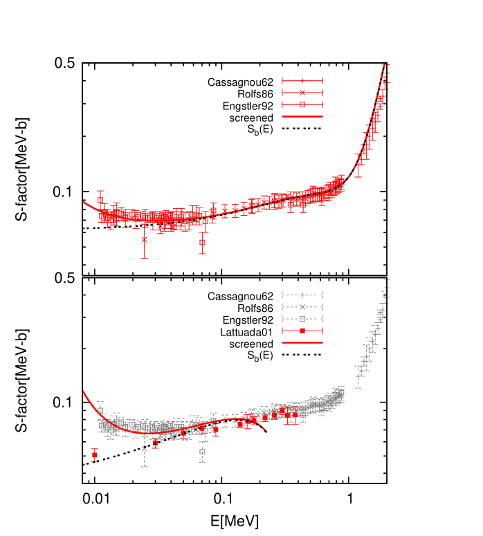
Figure 2: $S$-factor for the reaction ⁷Li($p,\alpha$)⁴He as a function of the incident c.m. energy. In the top panel experimental points are taken from cjmsf (Cassagnou62), from rk86 (Rolfs86), from erag ; erag-b (Engstler92). The solid curve represents our fit by polynomial expression with the adiabatic enhancement. The dashed curve corresponds to the bare $S$-factor. In the bottom panel the data from la01 (Lattuada01) are shown, together with other experimental data in the top panel. The solid curve represents our fit by using Eq.(5), instead of the polynomial expression, and with treating the screening potential as a parameter.

In Fig. 2 experimental data of the $S$-factor of the reaction ⁷Li($p,\alpha$)⁴He from several direct measurements are shown with error bars. We performed the fit of the data in the incident energy region from 0.01 MeV to 1 MeV using a cubic polynomial without enhancement factor. The obtained fitting parameters are shown in the third row of Table 4. This fitting procedure without enhancement factor is quite sensitive to the choice of both the upper and the lower limits of the fitting range.

Table 4: Fitting parameters of the reaction ⁷Li($p,\alpha$)⁴He. The three rows are obtained by using a cubic polynomial and from nacre  (the first row), with the adiabatic approximation(the second row), and without enhancement (the third row).

$S_{b}(0)$(MeVb)	$S_{1}$(b)	$S_{2}$(MeV-1b)	$S_{3}$(MeV-2b)	$U_{e}$(eV)	$\chi^{2}_{\nu}$
0.0593	0.193	-0.355	0.236	300
0.0620 $\pm$ 0.0006	0.15 $\pm$ 0.01	-0.24 $\pm$ 0.03	0.14 $\pm$ 0.03	175	0.41
0.0673 $\pm$ 0.0008	0.10 $\pm$ 0.01	-0.13 $\pm$ 0.04	0.08 $\pm$ 0.03	0	0.62

Table 5: Fitting parameters and the $S_{b}(0)$ of the reaction ⁷Li($p,\alpha$)⁴He using Eq. (5). The first row is obtained by using the screening potential 300 eV, the second row in the adiabatic limit, the third row without enhancement, and the last row is obtained by treating $U_{e}$ as a fitting parameter.

$\Pi_{1f}(0)$	$d_{1}$	$U_{e}$ (eV)	$\chi_{\nu}^{2}$	$S_{b}(0)$(MeVb)
7.1$\times$10-5	4.7	300	1.4	0.033
6.0$\times$10-5	4.9	175	2.1	0.035
5.0$\times$10-5	5.1	0	3.5	0.038
9.6$\times$10-5	4.3	495 $\pm$ 41	1.0	0.031

The experimental data from erag ; erag-b show the enhancement of the $S$-factor in the low-energy region. In the compilation NACRE nacre , authors used the screening potential $U_{e}=$ 300 (eV), which is larger than the adiabatic limit, and a cubic polynomial to obtain the $S$-factor. The fitting parameters in nacre are shown in the first row. However in the experiments erag ; erag-b LiF solid targets and deuteron projectiles as well as deuterium molecular gas targets and Li projectiles are utilized. In the case of LiF target, which is an ionic crystal similar to NaCl and a large band gap insulator, one can approximate the electronic structure of the target ⁷Li state by the ⁷Li⁺ with only two innermost electrons. Thus one expects the screening potential in the adiabatic limit $U^{(AD)}_{e}$ = 371.8-198.2$\sim$174 (eV). The best fit of the experimental data in the form of Eq. (8) and $U_{e}^{(AD)}=$ 175 (eV) kb-icfe gives the fitting parameters in the second row of Table 4 with the reduced $\chi^{2}=0.46$. The corresponding $S$-factor is shown with the dashed curve in Fig. 2. If we fit the same data by varying the screening potential $U_{e}$, we obtain $U_{e}=195\pm 28$ (eV) and $S_{b}(0)=$0.061$\pm$0.001 (MeVb), with $\chi^{2}_{\nu}=0.41$. This is, practically, consistent with the result (the second row of Table 4) in the adiabatic limit. $S_{b}(0)$ in the adiabatic limit is lower than the value obtained by the fit assuming no screening enhancement but higher than the value obtained in nacre where the authors used $U_{e}=$ 300 (eV). We have checked the sensitivity of $S_{b}(0)$ on the degree of the polynomial and the fitting range. Fixing the fitting range from the lowest experimental data 0.011MeV to 1MeV, we obtained $S_{b}(0)$=0.0620$\pm$0.0006 (MeVb) and 0.0617$\pm$0.0009 (MeVb), using a cubic polynomial and using a quartic polynomial, respectively. Both have $\chi_{\nu}^{2}$=0.41. Hence we choose a cubic polynomial for the following fit. In addition to this, assuming the adiabatic enhancement factor, the value $S_{b}(0)$ varies from 0.0620 (MeVb) to 0.0632 (MeVb), as one changes the fitting upper limit from 1 (MeV) to 0.5 (MeV) with fixing the lower limit 0.011 MeV. On the other hand $S_{b}(0)$ varies from 0.0620 (MeVb) to 0.578 (MeVb), as one changes the lower limit from 0.01 (MeV) to 0.04 (MeV). $S_{b}(0)$ obtained by using the polynomial expression is more sensitive to the choice of the lower limit than to the choice of the upper limit.

The fitting procedures of the same data but using Eq. (5) are performed. We have used only the $l=$1 partial-wave, because $l$ must be odd to obtain positive-parity state of ⁸Be barker2000 ; daacv . Using only the $l=$1 component, our fitting procedure gives a steeper incident energy dependence than the case where $l=$0 is used. In passing we mention briefly that the fitting procedure of the reaction ⁶Li($p$,$\alpha$)³He in the next subsection for a comparison. With the screening potential $U_{e}=$300, 175, 0 (eV) we obtain zero energy $S$-factors 0.033, 0.035, 0.038 (MeVb), respectively, as they are shown in Table 5. They are all considerably smaller than the results of polynomial fitting and $\chi_{\nu}^{2}$ of all cases are larger than the results of polynomial fitting. The radial parameters $d_{1}$ for all three cases are considerably larger than 1. This fact suggests that the interaction radius is 5 times larger than the empirical formula for the $l=$1 partial-wave. Again, if we fit the same data by varying the screening potential $U_{e}$, we obtain $U_{e}=495\pm 41$ (eV). The fitting parameters of this procedure are shown in the last row in Table 5. The curve obtained by this fitting procedure is shown in the bottom panel in Fig. 2. The extracted bare $S$-factor data by THM are especially shown with the closed squares la01 but these data are not included in the fitting procedure. Nevertheless the obtained bare $S$-factor curve follows the data by THM, which is thought to give the bare $S$-factor.

In Ref. daacv the $R$-matrix fitting for higher energy region ($E>40$ keV) has been used to determine the $S$-factor. They obtained the zero-energy $S$-factor 0.067 $\pm$ 0.004 (MeVb) and the screening potential $U_{e}=100\pm 25$ (eV), which is less than that within the adiabatic limit. The $S$-factor at zero energy from our results using polynomials $S_{b}(0)$=0.065 $\pm$ 0.005 (MeVb) and 0.0620 $\pm$ 0.0006 (MeVb) are in agreement with this result from the $R$-matrix fitting.

3.3 ⁶Li($p$,$\alpha$)³He

In contrast to the reaction ⁷Li($p$,$\alpha$)⁴He, the reaction ⁶Li($p$,$\alpha$)³He does not have the restriction on the incident partial-wave. For a comparison, we show the fitting curves of this reaction in Fig. 3, where the top panel shows the two curves from a fitting procedure using a polynomial and the bottom panel shows the curves obtained by using Eq. (5), although this reaction is not included in the PP-chains,

The fitting procedures of the experimental data using Eq. (5) are performed. Using the $l=$0 partial-wave alone, we obtain $S_{b}(0)=$ 3.3 (MeV), with $\chi^{2}_{\nu}$ =2.5 with fixing the screening potential $U_{e}$ = 175 (eV) in the adiabatic limit. We obtain $U_{e}$ = 466 $\pm$ 31 (eV) and $S_{b}(0)=$ 3.1 (MeV), with $\chi^{2}_{\nu}$ =1.4 by treating $U_{e}$ as a fitting parameter. The fitting parameters are shown in Table 6. For this reaction the radial parameter $d_{0}$ for all three cases are about unity. Although the screening potentials are different, the difference does not affect either the $S_{b}(0)$ or the fitting parameters, $\Pi_{0f}(0)$ and $d_{0}$. Only the $\chi^{2}_{\nu}$ for $U_{e}$ = 466 $\pm$ 31 (eV) is much smaller than the others. The obtained screening potential from the latter procedure is in agreement with one in the reaction ⁷Li($p$,$\alpha$)⁴He. This fact supports the isotopic independence of the electron screening.

Figure 3: $S$-factor for the reaction ⁶Li($p$,$\alpha$)³He as a function of the incident c.m. energy. The experimental points are from ma56 (Marion56), from ge66 (Gemeinhardt66), from sp71 (Spinka71), from el79 (Elwin79), from sh79 (Shinozuka79), from kw89 (Kwon89) and from erag (Engstler92). In the top panel the solid curve represents our fit by polynomial expression with the adiabatic enhancement. The dashed curve corresponds to the bare $S$-factor. In the bottom panel the solid curve represents our fit by using Eq. (5), instead of the polynomial expression, and with treating the screening potential as a parameter.

Table 6: Fitting parameters and the $S_{b}(0)$ of the reaction ⁶Li($p,\alpha$)³He by using fitting procedure Eq. (5). The first row is obtained by using the screening potential in the adiabatic limit, the second row corresponds to the zero screening potential, the last row is obtained by treating $U_{e}$ as a fitting parameter.

$\Pi_{0f}(0)$	$d_{0}$	$U_{e}$ (eV)	$\chi_{\nu}^{2}$	$S_{b}(0)$(MeVb)
0.11	1.2	175	2.5	3.3
0.11	1.2	0	3.8	3.5
0.12	1.1	466 $\pm$ 31	1.4	3.1

From the tree results of all the transfer reactions considered, ³He(³He,2$p$)⁴He, ⁷Li($p,\alpha$)⁴He, and ⁶Li($p$,$\alpha$)³He, one can say that the enhancement by the screening is crucial, in the sense that the fitting procedure without enhancement gives $\chi_{\nu}^{2}$ larger than the others. However the obtained $S_{b}(0)$ is insensitive to the magnitude of the screening potential.

3.4 D($p$,$\gamma$)³He

The $S$-factor data of the reaction D($p$,$\gamma$)³He from several measurements are shown with error bars in Fig. 4. We performed the fitting procedure of the data in the incident energy region from 0.0025 (MeV) to 1 (MeV) using a quadratic polynomial without enhancement factor. The obtained fitting parameters are shown in the second row of Table 7. In nacre the same polynomial degree has been used but the low-energy data by ca02 were not available at that time.

At the minimum incident energy in Ref. ca02 the screening enhancement is estimated to be 7% at utmost. This enhancement within the adiabatic limit is, again, estimated by using a linear combination of the even and odd states of the electronic wave function, reflecting the charge symmetry of the system as Eq. (15) where $U_{e}^{(AD)1}$ and $U_{e}^{(AD)2}$ are replaced by 40.8 eV and 0.0 eV, respectively.

Figure 4: $S$-factor for the reaction D($p$,$\gamma$)³He as a function of the incident c.m. energy. The experimental points are from gr62 (Griffiths62), from wa63 (Warren63), from be64 (Berman64), from wo67 (Wolfli67), from sc95 (Schmid95) and from ca02 (Casella02). In the top panel the solid curve represents our fit by polynomial expression with the adiabatic enhancement. The dashed curve corresponds to the bare $S$-factor. In the bottom panel the curves are same with ones in the top panel, but using Eq. (5) instead of the polynomial expression.

Table 7: Fitting parameters of the reaction D($p,\gamma$)³He. The three rows are obtained by using a quadratic polynomial and from nacre (the first row), without enhancement (the second row) and with the adiabatic approximation (the third row).

$S_{b}(0)$ (eVb)	$S_{1}$ (b)	$S_{2}$ (eV-1b)	$U_{e}$ (eV)	$\chi_{\nu}^{2}$
0.20$\pm$0.07	5.60$\pm$2.00	3.10$\pm$1.10	0.0	(NACRE)
0.261$\pm$0.006	1.3$\pm$0.2	12.0$\pm$1.0	0.0	2.7
0.256$\pm$0.006	1.4$\pm$0.2	11.8$\pm$1.0	40.8,0.0	3.9

Table 8: Fitting parameters and the $S_{b}(0)$ of the reaction D($p,\gamma$)³He by using the fitting procedure Eq. (5). The first and the second rows are obtained by the fitting without enhancement, and by using the screening potential $U_{e}$ in the adiabatic limit, respectively.

$\Pi_{0f}(0)$	$\Pi_{1f}(0)$	$d_{0}$	$d_{1}$	$U_{e}$ (eV)	$\chi_{\nu}^{2}$	$S_{b}(0)$ (eVb)
2.5$\times$10-8	3.4$\times$10-8	3.4	4.0	0.0	2.7	0.25
2.3$\times$10-8	3.6$\times$10-8	3.7	3.9	40.8, 0.0	2.8	0.25

The fitting parameters obtained using a quadratic polynomial with the adiabatic enhancement are shown in the third row in Table 7 and it is shown with the dashed curve in the top panel in Fig. 4. Because the enhancement is less than 7% even at the lowest measured incident energy, it changes insignificantly the zero-energy $S$-factor: $S(0)$=0.261 $\pm$ 0.006 (eVb) obtained by neglecting the enhancement differs only slightly from the bare $S$-factor at zero-energy $S_{b}(0)$= 0.256 $\pm$ 0.006 (eVb) from our fitting procedure. $S_{b}(0)$= 0.256 $\pm$ 0.006 (eVb) is slightly higher than the result from the $R$-matrix fit $S_{b}(0)$= 0.223$\pm$0.010 (eVb) in Ref. daacv , which is obtained as a sum of M1 and E1 contributions. Limiting the fitting range from 0.0025 MeV to 1 MeV, $S_{b}(0)$ is insensitive to the choice of the degree of the polynomial. However the $S_{b}(0)$ obtained using polynomials is quite sensitive to the choice of both the upper and the lower limits of the fitting range.

We performed the fitting procedures using Eq. (5). This fitting procedure without enhancement and with the adiabatic enhancement factor lead the fitting parameters and the $S_{b}(0)$ in Table 8. We have used the $l=$ 0 and 1 states. The obtained $S_{b}(0)$ are essentially the same for two cases and are in agreement with the extrapolations using quadratic polynomials. The radial parameters $d_{0}$ and $d_{1}$ for both cases are larger than one. This can be interpreted because the effective radius of deuteron is larger than the one given by the empirical formula. The curve obtained by this fitting procedure for the adiabatic enhancement is shown in the bottom panel in Fig. 4.

3.5 ³He($\alpha,\gamma$)⁷Be

The $S$-factor of the reaction ³He($\alpha$,$\gamma$)⁷Be has been investigated recently both by the activation bemmerer:122502 ; gyurky:035805 and the prompt methods confortola:065803 . The latter confirmed that there is no discrepancy between the obtained $S$-factors by two different methods. They have discussed the electron screening enhancement factor in the adiabatic limit in gyurky:035805 , but the $S$-factor data has not been corrected by the effect. The $S$-factor of the reaction ³He($\alpha,\gamma$)⁷Be from several measurements are shown with error bars in Fig. 5. The fitting parameters in nacre are shown in the first row of Table 9. The screening potential for the reaction ³He($\alpha,\gamma$)⁷Be is estimated in the same way with the reaction ³He(³He,2$p$)⁴He. The estimated enhancement at the minimum incident energy within the adiabatic limit is 2% at utmost.

Figure 5: $S$-factor for the reaction ³He($\alpha,\gamma$)⁷Be as a function of the incident c.m. energy. The experimental points are from pa63 (Parker63), from kr82 (Kraewinkel82), from os82 (Osborne82), from hi88 (Hilgemeier88), from bemmerer:122502 (Bemmerer06) and from confortola:065803 (Confortola07). In the top panel the solid curve represents our fit by polynomial expression with the adiabatic enhancement. The dashed curve corresponds to the bare $S$-factor. In the bottom panel the curves are same with ones in the top panel, but using Eq. (5) instead of the polynomial expression.

We performed the fit of the data in the incident energy region from 0.1072 MeV to 1 MeV using quadratic polynomials with the adiabatic enhancement factor. The obtained fitting parameters are shown in the second row of Table 9. We have performed the same fit but without enhancement factor and obtained the same $S_{b}(0)$ as the one with the adiabatic enhancement. The obtained $S_{b}(0)$ coincides with the one in nacre within the error. However $S_{b}(0)$ is rather sensitive to the choice of the fitting range, especially to the choice of the lower limit. $S_{b}(0)$ is insensitive to the choice of the degree of polynomial in the selected fitting range. In the top panel in Fig. 5 we have shown the results of the fitting using the adiabatic enhancement factor. The $S$-factor at zero-energy $S_{b}(0)$=0.49 $\pm$ 0.01 (keVb) from our procedure is in agreement with the result from the $R$-matrix fitting 0.51$\pm$0.04 (keVb) in Ref. daacv .

Table 9: Fitting parameters of the reaction ³He($\alpha,\gamma$)⁷Be. The two rows are obtained by using polynomial expression and from nacre  (the first row), with the adiabatic approximation (the second row).

$S_{b}(0)$ (keVb)	$S_{1}$ (b)	$S_{2}$ (keV-1b)	$U_{e}$ (eV)	$\chi_{\nu}^{2}$
0.54 $\pm$ 0.09	-0.52	-0.52	0.0	(NACRE)
0.50 $\pm$ 0.01	-0.35 $\pm$ 0.04	0.13 $\pm$ 0.03	246.8	0.0014

Table 10: Fitting parameters and the $S_{b}(0)$ of the reaction ³He($\alpha,\gamma$)⁷Be by using the fitting procedure Eq. (5). The first and the second rows are obtained by the fitting without enhancement, and by using the screening potential $U_{e}$ in the adiabatic limit, respectively.

$\Pi_{0f}(0)$	$\Pi_{2f}(0)$	$d_{0}$	$d_{2}$	$U_{e}$ (eV)	$\chi_{\nu}^{2}$	$S_{b}(0)$ (keVb)
5.1$\times$10-7	4.9$\times$10-7	4.0	2.5	0.0	2.3	0.51
5.3$\times$10-7	4.9$\times$10-7	4.0	2.5	246.8	2.3	0.50

The fitting parameters from the fitting procedures with Eq. (5) are shown in Table 10. We have used the $l=$0, 2 partial-wave contributions. This procedure using the enhancement factors with $U_{e}^{(AD)}=$ 246.8, 0.0 (eV) gives zero energy $S$-factors 0.50 and 0.51 (keVb), respectively. Both are in agreement with the result from the polynomial fitting procedure. The radial parameters $d_{0}$ and $d_{2}$ for both cases are larger than one. The curve obtained by this fitting procedure with the adiabatic enhancement is shown in the bottom panel in Fig. 5. The obtained zero energy $S$-factor is smaller than $S(0)=0.560\pm 0.017$ (keV) in confortola:065803 . This is because their result is obtained by a normalization to their data.

3.6 ⁷Be($p$,$\gamma$)⁸B

The reaction ⁷Be($p$,$\gamma$)⁸B is a key process to produce the high energy solar neutrinos through the $\beta$-decay of ⁸B. The $S$-factor of this reaction is investigated intensively by many groups by means of the direct capture (DC) reaction baby:065805 ; ju03 , the indirect Coulomb dissociation (CD) method PhysRevLett.83.2910 ; schumann:015806 and the asymptotic normalization coefficients (ANCs) trache:062801 . It was claimed that the experimental data of the $S$-factor by CD experiments gives a steeper energy dependence than that by DC experiments in the low-energy region and the lower zero-energy $S$-factor as an average ju03 . Recently this inconsistency has been resolved by reanalyzing data by the Coulomb dissociation method schumann:015806 .

Figure 6: $S$-factor for the reaction ⁷Be($p$,$\gamma$)⁸B as a function of the incident c.m. energy. The experimental points are from ju03 (Junghans03) and from schumann:015806 (Schuemann06). In the top panel the solid curve represents our fit by polynomial expression with the adiabatic enhancement. The dashed curve corresponds to the bare $S$-factor. In the bottom panel the curves are same with ones in the top panel, but using Eq. (5) instead of the polynomial expression.

For the purpose of the extrapolation of zero-energy $S$-factor, both the DC and the CD experiments above mentioned use the microscopic cluster model desc and give the zero-energy $S$-factor 22.1 $\pm$ 0.6(expt.) $\pm$ 0.6(theor.) (eVb) [$21.4\pm 0.5$(expt.) $\pm$ 0.6(theor.) (eVb) as a mean of all modern direct measurements] and 20.6 $\pm 0.8$ (stat.) $\pm$ 1.2 (syst.) (eVb), respectively. Let us remind you that the purpose of this paper is not a precise determination of the $S$-factor but to see the effect of the electron screening on the determination of the $S$-factor. So that we rather use the consistent approaches with the other reactions than employ a special treatment for this reaction. However we, at least, need to include the resonances to analyzing the DC data ju03 . For this purpose we use the Breit-Wigner formula Eq. (9). Moreover it is well known that this reaction has a low-energy bound state in the ⁸B PhysRevC.58.3711 ; PhysRevC.61.045801 . To take into account this state, we use

$$S_{b}(E)=\frac{S_{-1}}{E_{B}+E}+S_{0}+S_{1}E,$$ (16)

where $E_{B}=0.1375$ (MeV) PhysRevC.58.3711 , in place of the polynomial expression. We make a special mention of ⁷Be metallic target being used in the experiment ju03 . The experimental data of the $S$-factor in Ref. ju03 is fitted with the Breit-Wigner single-level resonance formula for 1⁺ and 3⁺ resonances plus Eq. (16). We use the resonance parameters in Ref. ju03 and obtained $S_{b}(0)=$ 20.8 (eVb) with $\chi_{\nu}^{2}=$0.3 from the fitting procedure without enhancement factor. Assuming the adiabatic enhancement, the screening enhancement factor is of the order of 1% at the minimum incident energy of the experiment in ju03 . By making use of the enhancement factor with the adiabatic screening potential $U_{e}^{(AD)}=$ 222.0 (eV), we obtain $S_{b}(0)=$ 20.5 (eVb) with $\chi_{\nu}^{2}=$0.3. The corresponding bare $S$-factor is shown with the dashed curve in the top panel in Fig. 6. The difference between two $S_{b}(0)$ using different screening potentials is less than 2%. Considering the isotopic independence of the electron screening, we, tentatively, use the screening potential obtained by the measurement of the reaction ⁹Be($p,\alpha$)⁶Li: $U_{e}$=900$\pm$50 (eV) zahnow . The fitting procedure gives $S_{b}(0)=$ 19.7 (eVb) with $\chi_{\nu}^{2}=$ 0.3. This is 4% smaller than the former two results. We summarize the fitting parameters in above fitting procedures in Table 11.

Table 11: Fitting parameters and $S_{b}(0)$ of the reaction ⁷Be($p$,$\gamma$)⁸B by using the polynomial Eq. (16). The four rows are obtained from nacre (the first row), without enhancement (the second row), with the adiabatic approximation (the third row), and with the screening potential $U_{e}$= 900 (eV) zahnow  (the fourth row).

$S_{-1}$ (eV2b)	$S_{0}$ (eVb)	$S_{1}$ (b)	$S_{2}$	$U_{e}$ (eV)	$\chi^{2}_{\nu}$	$S_{b}(0)$
	21. $\pm$ 2.	18.	38.	0.0	(NACRE)	21. $\pm$ 2.
0.6 $\pm$ 0.2	15.7 $\pm$ 0.6	8.3 $\pm$ 0.4		0.0	0.3	20.8
0.7 $\pm$ 0.2	15.7 $\pm$ 0.6	8.3 $\pm$ 0.4		222.0	0.3	20.5
0.7 $\pm$ 0.2	16.0 $\pm$ 0.6	8.1 $\pm$ 0.4		900.0	0.3	19.7

Table 12: Fitting parameters and the $S_{b}(0)$ of the reaction ⁷Be($p,\gamma$)⁸B by using the fitting procedure Eq. (5) with resonant terms. The three rows are obtained by the fitting without enhancement (the first), and by using the screening potential $U_{e}$ in the adiabatic limit (the second), and with the screening potential $U_{e}$= 900 (eV) (the third), respectively.

$\Pi_{0f}(0)$	$\Pi_{2f}(0)$	$d_{0}$	$d_{2}$	$U_{e}$ (eV)	$\chi_{\nu}^{2}$	$S_{0}$ (eVb)
2.2$\times$10-8	2.5$\times$10-4	0.9	0.2	0.0	0.4	22.4
2.2$\times$10-8	2.3$\times$10-4	0.9	0.2	222.	0.4	22.3
2.2$\times$10-8	2.0$\times$10-4	0.9	0.2	900.	0.5	22.1

We perform the fitting procedures of the experimental data in Ref. ju03 using Eq. (5) including 1⁺ and 3⁺ resonances plus another resonance with negative energy -0.1375 (MeV), which corresponds to the pole term in Eq. (16).

$$S_{b}(E) = \frac{\pi\hbar^{2}}{2\mu}(\Pi_{0f}(E)e^{W_{0}}+5\Pi_{2f}(E)e^{W_{2}})$$ (17)

$$+ \frac{c_{r1}e^{W_{0}}\Pi_{0f}(E)}{(E+0.1375)^{2}}+\frac{c_{r2}e^{W_{0}}\Pi_{0f}(E)}{(E-0.630)^{2}+\Gamma^{2}/4}+\frac{c_{r3}e^{W_{2}}\Pi_{2f}(E)}{(E-2.183)^{2}+\Gamma^{2}/4}$$

where $c_{r1},c_{r2}$ and $c_{r3}$ are scaling factors in Eq. (10). Our fitting procedures using different screening potentials give common $c_{r1}=5.\times 10^{-7}$ (MeV²), $c_{r2}=2.\times 10^{-9}$(MeV²) and $c_{r1}=2.\times 10^{-6}$ (MeV²). In the bottom panel of Fig. 6 the thin dotted and dot-dashed curves show the contributions from resonances, including the negative-energy resonance, and the non-resonant part, respectively. We have used the $l=$ 0 and 2 partial-waves.

The fitting procedure using Eq. (17) without enhancement, with the adiabatic enhancement factor, and with $U_{e}$= 900 (eV) lead the fitting parameters and the $S_{b}(0)$ in Table 12. Despite of the difference of the utilized screening potentials, neither the obtained zero-energy $S$-factor nor $\chi_{\nu}^{2}$ does have much differences. The values $\Pi_{2f}(0)$ are much larger than $\Pi_{0f}(0)$, i.e., the $d$-wave contribution is dominant in the energy region investigated. The radial parameter $d_{0}$ is smaller than one, and $d_{1}$ is smaller than $d_{0}$ for all three cases. The curve obtained by this fitting procedure for the adiabatic enhancement is shown in the bottom panel in Fig. 6. The obtained $S_{b}(0)$ using different screening potentials are in accordance with the result with the microscopic cluster model desc $S_{b}$(0)=22.1 $\pm$ 0.6(expt.) $\pm$ 0.6(theor.) (eVb) in Ref. ju03 within the error-bar.

From the tree results of all the radiative capture reactions considered, D($p$,$\gamma$)³He, ³He($\alpha,\gamma$)⁷Be, and ⁷Be($p,\gamma$)⁸B, one can say that the obtained $S_{b}(0)$ is insensitive if the screening enhancement, within the adiabatic approximation, is taken into account or not. For all the reactions investigated in this paper the fitting procedure with the polynomial expression is more sensitive to the difference of the screening potential than the fitting procedure with Eq. (5).

4 Conclusions

We discussed the bound electron screening corrections to the bare $S$-factors of the reactions in PP-chains. Our approach is based on fitting procedures of the experimental data. For this purpose we employed two different fitting procedures: one is the conventional polynomial expressions and the other includes explicitly the contribution of the nuclear interaction and based on the statistical model to describe exit channels. The later fitting procedure works especially well for the reactions that have a dominant $s$-wave entrance channel component. We have applied different types of screening enhancements: in the adiabatic limit, determined through a fit and larger than adiabatic screening potentials, as well. From the tree results of all the transfer reactions considered, ³He(³He,2$p$)⁴He, ⁷Li($p,\alpha$)⁴He, and ⁶Li($p$,$\alpha$)³He, the enhancement by the screening is crucial, in the sense that the fitting procedure without enhancement gives $\chi_{\nu}^{2}$ larger than the others in which the screening enhancement is taken into account. However the obtained $S_{b}(0)$ is insensitive to the magnitude of the screening potential. Especially for the radiative capture reactions D($p$,$\gamma$)³He and ⁷Be($p,\gamma$)⁸B, the screening correction within the adiabatic approximation has been considered for the first time. However the results suggest that the obtained $S_{b}(0)$ is insensitive whether the screening enhancement, within the adiabatic approximation, is taken into account or not. Making a comparative study of the bare $S$-factors obtained by two-ways of fitting procedures using different screening enhancement factors, we found that all $S_{b}(E)$ coincide within the standard errors. $S_{b}(E)$ is, practically, insensitive to the magnitude of the screening potential.

The authors acknowledge Prof. S. Kubono for the suggestion of the problem and valuable comments. One of us (S. K.) thanks Dr. H. Costantini and Dr. R. G. Pizzone for stimulating discussions and for providing us experimental data.

References

- (1) C. Angulo, M. Arnould, M. Rayet, P. Descouvemont, D. Baye, C. Leclercq-Willain, A. Coc, S. Barhoumi, P. Aguer, C. Rolfs, R. Kunz, J.W. Hammer, A. Mayer, T. Paradellis, S. Kossionides, C. Chronidou, K. Spyrou, S. Degl’Innocenti, G. Fiorentini, B. Ricci, S. Zavatarelli, C. Providencia, H. Wolters, J. Soares, C. Grama, J. Rahighi, A. Shotter, and M. Lamehi Rachti. Nucl. Phys. A, 656:3, 1999.
- (2) D. D. Clayton. Principles of Stellar Evolution and Nucleosynthesis. University of Chicago Press, 1983.
- (3) G. Fiorentini, C. Rolfs, F. L. Villante, and B. Ricci. Phys. Rev. C, 67:014603, 2003.
- (4) J. Kasagi. Prog. Theor. Phys. Sup., 154:365, 2004.
- (5) F. Raiola and P. Migliardi and L. Gang and C. Bonomo and G. Gyürky and R. Bonetti and C. Broggini and N.E. Christensen and P. Corvisiero and J. Cruz and A. D’Onofrio and Z. Fülöp and G. Gervino L. Gialanella and A.P. Jesus and M. Junker K. Langanke and P. Prati and V. Roca C. Rolfs and M. Romano and E. Somorjai and F. Strieder and A. Svane F. Terrasi and J. Winter. Phys. Lett. B, 547:193, 2002.
- (6) F. Raiola and B. Burchard and Z. Fülöp and G. Gyürky and S. Zeng and J. Cruz and A. Di Leva and B. Limata and M. Fonseca and H. Luis and M. Aliotta and H. W. Becker and C. Broggini and A. D’Onofrio and L. Gialanella and G. Imbriani and A. P. Jesus and M. Junker and J. P. Ribeiro and V. Roca and C. Rolfs and M. Romano and E. Somorjai and F. Strieder and F. Terrasi. J. Phys. G, 31:1141, 2005.
- (7) J. Cruz and Z. Fülöp and G. Gyürky and F. Raiola and A. Di Leva and B. Limata and M. Fonseca and H. Luis and D. Schuermann and M. Aliotta and H.W. Becker and A.P. Jesus and K.U. Kettner and J.P. Ribeiro and C. Rolfs and M. Romano and E. Somorjai and F. Strieder. Phys. Lett. B, 624:181, 2005.
- (8) G. Shaviv and N. Shaviv. Astrophys. J, 529:1054, 2000.
- (9) S. Ichimaru. Rev. Mod. Phys., 65:255, 1993.
- (10) Y. Kato and N. Takigawa. Physical Review C, 76:014615, 2007.
- (11) V. N. Kondratyev and A. Bonasera. Phys. Rev. Lett., 74:2824, 1995.
- (12) H. J. Assenbaum, K. Langanke, and C. Rolfs. Z. Phys. A, 327:461, 1987.
- (13) T. D. Shoppa, S. E. Koonin, K. Langanke, and R. Seki. Phys. Rev. C, 48:837, 1993.
- (14) S. Kimura, N. Takigawa, M. Abe, and D.M. Brink. Phys. Rev. C, 67:022801(R), 2003.
- (15) M. Papa, T. Maruyama, and A. Bonasera. Phys. Rev. C, 64:024612, 2001.
- (16) S. Kimura and A. Bonasera. Phys. Rev. A, 72:014703, 2005.
- (17) S. Kimura and A. Bonasera. Phys. Rev. Lett., 93:262502, 2004.
- (18) S. Kimura and A. Bonasera. Nucl. Phys. A, 759:229, 2005.
- (19) C. Angulo and P. Descouvemont. Nucl. Phys. A, 639:733, 1998.
- (20) F. C. Barker. Nucl. Phys. A, 707:277, 2002.
- (21) P. Descouvemont, A. Adahchour, C. Angulo, A. Coc, and E. Vangioni-Flam. Atomic Data and Nuclear Data Tables, 88:203, 2004.
- (22) D. Baye and E. Brainis. Phys. Rev. C, 61:025801, 2000.
- (23) V. Weisskopf. Phys. Rev., 52:295, 1937.
- (24) A. Bonasera, M. Di Toro, and C. Gregoire. Nucl. Phys. A, 483:738, 1988.
- (25) A. Bonasera and G.F. Bertsch. Phys. Lett. B, 195:521, 1987.
- (26) S. Kimura and A. Bonasera. Phys. Rev. C, 76:031602(R), 2007.
- (27) Gy. Gyürky, E. Somorjai, Zs. Fülöp, S. Harissopulos, P. Demetriou, and T. Rauscher. Phys. Rev. C, 64:065803, 2001.
- (28) M. Junker, A. D’Alessandro, S. Zavatarelli, C. Arpesella, E. Bellotti, C. Broggini, P. Corvisiero, G. Fiorentini, A. Fubini, G. Gervino, U. Greife, C. Gustavino, J. Lambert, P. Prati, W.S. Rodney, C. Rolfs, F. Strieder, H.P. Trautvetter, and D. Zahnow. Phys.Rev. C, 57:2700, 1998.
- (29) S. Engstler, G. Raimann, C. Angulo, U. Greife, C. Rolfs, U. Schröder, E. Somorjai, B. Kirch, and K. Langanke. Z. Phys. A, 342:471, 1992.
- (30) S. Engstler, G. Raimann, C. Angulo, U. Greife, C. Rolfs, U. Schröder, E. Somorjai, B. Kirch, and K. Langanke. Phys. Lett. B, 279:20, 1992.
- (31) John N. Bahcall, Walter F. Huebner, Stephen H. Lubow, Peter D. Parker, and Roger K. Ulrich. Rev. Mod. Phys., 54:767, 1982.
- (32) D. Bemmerer, F. Confortola, H. Costantini, A. Formicola, Gy. Gyürky, R. Bonetti, C. Broggini, P. Corvisiero, Z. Elekes, Z. Fülöp, G. Gervino, A. Guglielmetti, C. Gustavino, G. Imbriani, M. Junker, M. Laubenstein, A. Lemut, B. Limata, V. Lozza, M. Marta, R. Menegazzo, P. Prati, V. Roca, C. Rolfs, C. Rossi Alvarez, E. Somorjai, O. Straniero, F. Strieder, F. Terrasi, and H. P. Trautvetter. Phys. Rev. Lett., 97(12):122502, 2006.
- (33) Gy. Gyürky, F. Confortola, H. Costantini, A. Formicola, D. Bemmerer, R. Bonetti, C. Broggini, P. Corvisiero, Z. Elekes, Zs. Fülöp, G. Gervino, A. Guglielmetti, C. Gustavino, G. Imbriani, M. Junker, M. Laubenstein, A. Lemut, B. Limata, V. Lozza, M. Marta, R. Menegazzo, P. Prati, V. Roca, C. Rolfs, C. Rossi Alvarez, E. Somorjai, O. Straniero, F. Strieder, F. Terrasi, and H. P. Trautvetter LUNA Collaboration. Physical Review C, 75:035805, 2007.
- (34) F. Confortola, D. Bemmerer, H. Costantini, A. Formicola, Gy. Gyürky, P. Bezzon, R. Bonetti, C. Broggini, P. Corvisiero, Z. Elekes, Zs. Fülöp, G. Gervino, A. Guglielmetti, C. Gustavino, G. Imbriani, M. Junker, M. Laubenstein, A. Lemut, B. Limata, V. Lozza, M. Marta, R. Menegazzo, P. Prati, V. Roca, C. Rolfs, C. Rossi Alvarez, E. Somorjai, O. Straniero, F. Strieder, F. Terrasi, and H. P. Trautvetter. Physical Review C, 75:065803, 2007.
- (35) L. T. Baby, C. Bordeanu, G. Goldring, M. Hass, L. Weissman, V. N. Fedoseyev, U. Koster, Y. Nir-El, G. Haquin, H. W. Gaggeler, and R. Weinreich. Phys. Rev. C, 67(6):065805, 2003.
- (36) A. R. Junghans, E. C. Mohrmann, K. A. Snover, T. D. Steiger, E. G. Adelberger, J. M. Casandjian, H. E. Swanson, L. Buchmann, S. H. Park, A. Zyuzin, and A. M. Laird. Phys. Rev. C, 68:065803, 2003.
- (37) N. Iwasa, F. Boué, G. Surówka, K. Sümmerer, T. Baumann, B. Blank, S. Czajkowski, A. Förster, M. Gai, H. Geissel, E. Grosse, M. Hellström, P. Koczon, B. Kohlmeyer, R. Kulessa, F. Laue, C. Marchand, T. Motobayashi, H. Oeschler, A. Ozawa, M. S. Pravikoff, E. Schwab, W. Schwab, P. Senger, J. Speer, C. Sturm, and A. Surowiec. Phys. Rev. Lett., 83:2910, 1999.
- (38) H. Esbensen, G. F. Bertsch, and K. A. Snover. Phys. Rev. Lett., 94(4):042502, 2005.
- (39) F. Schumann, S. Typel, F. Hammache, K. Summerer, F. Uhlig, I. Bottcher, D. Cortina, A. Forster, M. Gai, H. Geissel, U. Greife, E. Grosse, N. Iwasa, P. Koczon, B. Kohlmeyer, R. Kulessa, H. Kumagai, N. Kurz, M. Menzel, T. Motobayashi, H. Oeschler, A. Ozawa, M. Ploskon, W. Prokopowicz, E. Schwab, P. Senger, F. St rieder, C. Sturm, Zhi-Yu Sun, G. Surowka, A. Wagner, and W. Walus. Phys. Rev. C, 73:015806, 2006.
- (40) A. D. Backer and T. A. Tombrello. Astrophysical Problems in “Nuclear research with Low-Energy Accelerators. Academic Press, 1967.
- (41) M. R. Dwarakanath and H. Winkler. Phys. Rev. C, 4:1532, 1971.
- (42) H. P. Trautvetter A. Krauss, H. W. Becker and C. Rolfs. Nucl. Phys. A, 467:273, 1987.
- (43) W. Lichten. Phys. Rev., 131:229, 1963.
- (44) Y. Cassagnou, J. M. Jeronymo, G. S. Mani, A. Sadeghi, and P. D. Forsyth. Nucl. Phys., 33:449, 1962.
- (45) C. Rolfs and R. W. Kavanagh. Nucl. Phys. A, 455:179, 1986.
- (46) M. Lattuada, R. G. Pizzone, S. Typel, P. Figuera, D. Miljani, A. Musumarra, M. G. Pellegriti, C. Rolfs, C. Spitaleri, and H. H. Wolter. Astrophys. J., 562:1076, 2001.
- (47) F. C. Barker. Phys. Rev. C, 62:044607, 2000.
- (48) J. B. Marion, G. Weber, and F. S. Mozer. Phys. Rev., 104:1402, 1956.
- (49) W. Gemeinhardt, D. Kamke, and C. von Rhoeneck. Z. Phys., 97:58, 1966.
- (50) H. Spinka, T. Tombrello, and H. Winkler. Nucl. Phys. A, 164:1, 1971.
- (51) A. J. Elwyn, R. E. Holland, C. N. Davids, L. Meyer-Schutzmeister, F. P. Mooring, and W. Ray Jr. Phys. Rev. C, 20:1984, 1979.
- (52) T. Shinozuka, Y. Tanaka, and K. Sugiyam. Nucl. Phys. A, 326:47, 1979.
- (53) J. U. Kwon, J. C. Kim, and B. N. Sung. Nucl. Phys. A, 493:112, 1989.
- (54) C. Casella and H. Costantini and A. Lemut and B. Limata and R. Bonetti and C. Broggini and L. Campajola and P. Corvisiero and J. Cruz and A. D’Onofrio and A. Formicola and Z. Fülöp and G. Gervino and L. Gialanella and A. Guglielmetti and C. Gustavino and G. Gyürky and G. Imbriani and A.P. Jesus and M. Junker and A. Ordine and J. Pinto and P. Prati and J.P.Ribeiro and V. Roca and D. Rogalla and C. Rolfs and M. Romano and C. Rossi-Alvarez and F. Schuemann and E. Somorjai and O. Straniero and F. Strieder and F. Terrasi and H.P. Trautvetter and S. Zavatarelli. Nucl. Phys. A, 706:203, 2002.
- (55) G.M. Griffiths, E.A. Larson, and L.P. Robertson. Can. J. Phys., 40:402, 1962.
- (56) J.B. Warren, K.L. Erdman, L.P. Robertson, D.A. Axen, and J.R. MacDonald. Phys. Rev., 132:1691, 1963.
- (57) B.L. Berman, L.J. Koester Jr., and J.H. Smith. Phys. Rev., 133:B117, 1964.
- (58) W. Wolfli, R. Bosch, J. Lang, R. Muller, and P. Marmier. Helv. Phys. Acta, 40:946, 1967.
- (59) G.J. Schmid, R.M. Chastler, C.M. Laymon, and H.R. Weller. Phys. Rev. C, 52, 1995.
- (60) P.D. Parker and R.W. Kavanagh. Phys. Rev., 131:2578, 1963.
- (61) H. Kraewinkel, H. W. Becker, L. Buchmann, J. Goerres K. U. Kettner, W.E . Kieser, R. Santo, P. Schmalbrock, H. P. Trauttvetter, A. Vielks, C. Rolfs, J. W. Hammer, R. E. Azuma, and W. S. Rodney. Z. Phys. A, 304:307, 1982.
- (62) J. L. Osborne, C. A. Barnes, R. W. Kavanagh, R. M. Kremer, G. J. Mathews, J. L. Zyskind, P. D. Parker, and A. J. Howard. Phys. Rev. Lett., 48:1664, 1982.
- (63) M. Hilgemeier, H. W. Becker, C. Rolfs, H. P. Trautvetter, and J. W. Hammer. Z. Phys. A, 329:243, 1988.
- (64) L. Trache, A. Azhari, F. Carstoiu, H. L. Clark, C. A. Gagliardi, Y.-W. Lui, A. M. Mukhamedzhanov, X. Tang, N. Timofeyuk, and R. E. Tribble. Phys. Rev. C, 67:062801, 2003.
- (65) P. Descouvemont. Phys. Rev. C, 70:065802, 2004.
- (66) B. K. Jennings, S. Karataglidis, and T. D. Shoppa. Phys. Rev. C, 58:3711, 1998.
- (67) M. Ueda, A. J. Sargeant, M. P. Pato, and M. S. Hussein. Phys. Rev. C, 61:045801, 2000.
- (68) D. Zahnow, C. Rolfs, S. Schmidt, and H.P. Trautvetter. Z.Phys.A, 359:211, 1997.