$p_{T}$-fluctuations and multiparticle clusters in heavy-ion collisions

Abstract:

We investigate the centrality dependence of the $p_{T}$-correlations in the event-by-event analysis of relativistic heavy-ion collisions at RHIC made recently by the PHENIX and STAR Collaborations. We notice that $\sigma^{2}_{\rm dyn}$ scales to a very good accuracy with the inverse number of the produced particles, $n$. This scaling can be naturally explained by formation of clusters. We discuss the nature of clusters and provide numerical estimates of correlations coming from resonance decays, which are tiny, and a model where particle are emitted from local thermalized sources moving at the same collective velocity. This ”lumped cluster” model can explain the data when on the average 6-15 particles are contained in a cluster. We also point out simple relations of the popular correlation measures to the covariance, which arise under the assumptions (well holding at RHIC) that the distributions are sharply peaked in $n$ and that the dynamical compared to statistical fluctuations are small.

1 Introduction

We have had very interesting presentations on event-by-event fluctuations during this workshop (see other contributions to these proceedings). This work is based on our recent paper [1] and explores from a theoretical viewpoint the correlation data published by the PHENIX [2, 3], STAR [4, 5], and CERES [6] Collaborations. These measurements contribute to the previously accumulated vast knowledge on event-by-event fluctuations in ultra-relativistic heavy-ion collisions [7, 8, 9, 10, 11, 12, 13, 14, 15, 6, 16, 17, 18, 19, 20, 21, 22, 23, 24, 25, 26, 27, 28, 31, 29, 30].

We bring up some basic and rather striking facts manifest in the data of Refs. [2, 5] and discuss their relevance to the cluster picture of correlations. Let us begin with the PHENIX measurement [2] of the event-by-event fluctuations of the transverse momentum at $\sqrt{s_{NN}}=130$ GeV. In order to simplify the notation, $p$ is used generically to denote the transverse momentum, $|\vec{p}_{T}|$ and $p_{i}$ is the value of $p$ for the $i$th particle. Finally, $M=\sum_{i=1}^{n}p_{i}/n$ is the average transverse momentum in an event of multiplicity $n$. The statistical treatment of the $M$ variable has been presented in detail in the contribution of the speaker to the discussion session (see “Round Table Discussion: Correlations and Fluctuations in Nuclear Collisions” in these proceedings [32]). For the reader’s convenience this material is inluded here in Appendix A.

2 A look at the data

The PHENIX results of Ref. [2] are reminded in Table 1.

Table 1: Data for the event-by-event fluctuations in the transverse momentum. Upper rows: the PHENIX measurement at $\sqrt{s_{NN}}=130$ GeV [2]. Bottom rows: the mixed-event results.

centrality	0-5%	0-10%	10-20%	20-30%
$\bar{n}$	59.6	53.9	36.6	25.0
$\sigma_{n}$	10.8	12.2	10.2	7.8
$\bar{M}$	523	523	523	520
$\sigma_{p}$	290	290	290	289
$\sigma_{M}$	38.6	41.1	49.8	61.1
$\bar{M}^{\rm mix}$	523	523	523	520
$\sigma_{M}^{\rm mix}$	37.8	40.3	48.8	60.0

Several important features of the data are immediately seen: firstly, the quantities $\bar{M}$, the average $p$ in a given centrality class, and $\sigma_{p}$, the inclusive standard deviation of $p$, are practically constant in the reported “fiducial centrality range” $c=0-30$%.

$$\bar{M}=\hbox{const.}\,,\;\;\;\;\;\sigma_{p}=\hbox{const.}~{}~{}(\rm{at~{}low}~{}c).$$ (1)

This allows us to replace the average momentum at each $n$ by $\bar{M}$ and the variance at each $n$ by $\sigma_{p}$ [1]. For distributions sharply peaked in the $n$ variable we derive in [32] the following formula:

$$\sigma_{M}^{\rm mix}\simeq\sigma_{p}/\sqrt{\bar{n}}.$$ (2)

The derivation involves only the statistics and the assumption of sharp distributions, which is sufficiently well satisfied at RHIC. Corrections to Eq. (2) appearing for broader distributions can be obtained. They involve higher moments of $n$, for instance $\sigma^{2}(n)/{\bar{n}}^{2}$. Table 2 shows how well (2) works – at the level of 1-2%, which is no wonder, just the statistical fact.

Table 2: Verification of the statistical result (2.2) holding for sharp distributions.

centrality	0-5%	0-10%	10-20%	20-30%
$\sigma_{M}^{\rm mix}$	37.8	40.3	48.8	60.0
$\sigma_{p}/\sqrt{\bar{n}}$	37.6	39.5	47.9	59.0

3 The cluster scaling

Next, we look at the difference of the measured and mixed-event variances of $M$, which is a measure of dynamical fluctuations,

$$\sigma_{\rm dyn}^{2}\equiv\sigma_{M}^{2}-\sigma_{M}^{2,{\rm mix}}.$$ (3)

Table 3 shows our main observation, namely, that the following scaling holds:

$$\sigma_{\rm dyn}\sim\frac{1}{\sqrt{\bar{n}}}.$$ (4)

It works at the accuracy level of 2% in the available centrality range, as can be inferred from the approximate constancy of numbers displayed in Table 3.

Table 3: Verification of the scaling result (3.2), seen in the approximate constancy of $\sigma_{\rm dyn}\sqrt{\bar{n}}$.

centrality	0-5%	0-10%	10-20%	20-30%
$\sigma_{\rm dyn}\sqrt{\bar{n}}$	$60.3\pm 1.6$	$59.2\pm 1.5$	$59.8\pm 1.2$	$57.7\pm 1.1$

Elementary statistical considerations shown in [32] lead to the result

$$\sigma_{\rm dyn}^{2}=\sum_{n}\frac{P(n)}{n^{2}}\sum_{i,j=1,j\neq i}^{n}{\rm cov}_{n}(p_{i},p_{j})\simeq\frac{1}{\bar{n}^{2}}\sum_{i,j=1,j\neq i}^{\bar{n}}{\rm cov}_{\bar{n}}(p_{i},p_{j}),$$ (5)

where in the second equality we have used the feature of sharp distributions in $n$. The quantity ${\rm cov}_{n}(p_{i},p_{j})$ is the covariance of momenta $p_{i}$ and $p_{j}$ in events of multiplicity $n$.

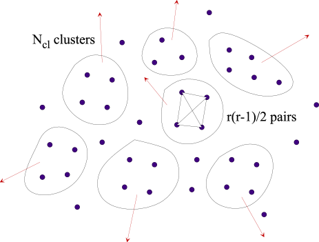
Figure 1: The cluster picture of correlations consistent with scaling (1.4).

Now we come to the physics discussion. The scaling (4) imposes severe constraints on the physics nature of the covariance term. For instance, if all particles were correlated to each other, then $\sum_{i,j=1,j\neq i}^{n}{\rm cov}_{\bar{n}}(p_{i},p_{j})$ would be proportional to the number of all pairs, and $\sigma_{\rm dyn}$ would be independent of $\bar{n}$. Thus we see that the combinatorics is truncated – clearly not all pairs are correlated, or a finite correlation length develops. A natural explanation of the scaling (4) comes from the cluster model, depicted in Fig. 1. The system is assumed to have $N_{\rm cl}$ clusters, each containing (on the average) $\langle r\rangle$ particles. The particles are correlated if and only if they belong to the same cluster, where the average covariance per pair is $2\,{\rm cov}^{\ast}$. The number of correlated pairs within a cluster is $r(r-1)/2$. Some particles may be unclustered, hence the ratio of clustered to all particles is $\langle N_{\rm cl}\rangle\langle r\rangle/{\bar{n}}=\alpha$. If all particles are clustered then $\alpha=1$. With these assumptions Eq. (3) becomes

$$\sigma_{\rm dyn}^{2}=\frac{\alpha\langle r(r-1)\rangle}{\langle r\rangle\bar{n}}{\rm cov}^{\ast}=\frac{\alpha r^{\ast}}{\bar{n}}{\rm cov}^{\ast},$$ (6)

where we have introduced $r^{\ast}=\langle r(r-1)\rangle/\langle r\rangle$, the ratio of the average number of pairs in the cluster to the average multiplicity of the cluster. For a fixed number of particles in each cluster we have $r^{\ast}=\langle r\rangle-1$, for the Poisson distribution $r^{\ast}=\langle r\rangle$, while for wider distributions $r^{\ast}>\langle r\rangle$. Equation (6) complies to the scaling (4) as long as the product $\alpha r^{\ast}{\rm cov^{\ast}}$ does not depend on $\bar{n}$ (in the fiducial centrality range). This is the basic physics constraint that follows from the data. For the reasons discussed above it is appropriate to term the scaling (4) the cluster scaling.

4 Cluster scaling with other correlation measures

There are numerous quantities used as measure of the event-by-event fluctuations. Fortunately, as shown in [32], for sharp distributions and for the case where the dynamical correlations are small compared to the statistical correlations, $\sigma_{\rm dyn}\ll\sigma_{M}$, all the popular measures are simply related to each other, or to the covariance, which is the basic quantity designed to describe correlations. We have

$$\Sigma^{2}_{p_{T}} \equiv {\sigma^{2}_{\rm dyn}}/{\overline{p}^{2}}\simeq\frac{\sum_{i\neq j}{\rm cov}_{\overline{n}}(p_{i},p_{j})}{{\bar{p}}^{2}{\bar{n}}^{2}},$$

$$F_{p_{T}} \equiv \frac{\sigma_{M}}{\sigma^{{\rm mix}}_{M}}-1=\sqrt{1+\frac{\sigma^{2}_{\rm dyn}}{\sigma^{2,{\rm mix}}_{M}}}-1\simeq\frac{1}{2}\frac{\sigma^{2}_{\rm dyn}}{\sigma^{2,{\rm mix}}_{M}}\simeq\frac{\sum_{i\neq j}{\rm cov}_{\overline{n}}(p_{i},p_{j})}{2{\bar{n}}\sigma_{p}^{2}},$$

$$\Phi_{p_{T}} \equiv \sqrt{\frac{\sigma_{S}^{2}}{\overline{n}}}-\sigma_{p}\simeq\frac{\sum_{i\neq j}{\rm cov}_{\overline{n}}(p_{i},p_{j})}{2\overline{n}\sigma_{p}},$$

$$\langle\Delta p_{i}\Delta p_{j}\rangle \equiv \sum_{i\neq j}{\rm cov}_{\overline{n}}(p_{i},p_{j}),$$ (7)

where in the definition of $\Phi_{p_{T}}$ one uses $S_{n}=p_{1}+\dots+p_{n}$. The last equality states the fact that the STAR measure $\Delta p_{i}\Delta p_{j}$ is just the statistical estimator of the covariance, see [1]. The cluster scaling thus manifests itself for the various measures in the following manner:

$$\Sigma_{p_{T}} \sim \frac{1}{\sqrt{\bar{n}}},$$

$$F_{p_{T}} \sim 1,$$

$$\Phi_{p_{T}} \sim 1,$$

$$\bar{n}\langle\Delta p_{i}\Delta p_{j}\rangle \sim 1.$$ (8)

Since this is an important point, we stress again: since at RHIC the distributions are 1) sufficiently sharply peaked in $n$ and 2) the dynamical fluctuations are small compared to the statistical fluctuations, all popular measures of event-by-event fluctuations are all proportional to each other and to the covariance. One may pass from one measure to another without difficulty. If conditions 1) and 2) are not satisfied, as may be the case at lower energies, periferal collisions, etc., then of course the measures remain different and some may be better tuned for certain analyses. Full information on correlations could be acquired by simply evaluating the covariance $\sum_{i\neq j}{\rm cov}_{n}$ separately for each $n$. Even if 1) or 2) are relaxed, the correlation measures are still related to the sum of the weighted covariances at various $n$, with the weights dependent on the particular measure. The necessary formulas can be very straightforwardly derived along the lines of [32]. We urge that such a study of the dependence of covariance on $n$ be made on data with sufficiently large samples.

5 Cluster scaling in various experiments

Now let us have a look at various experiments. The PHENIX results at $\sqrt{s_{NN}}=130$ GeV [2] discussed in Sect. 3 comply nicely to the cluster scaling. The same is true of the STAR data (see Fig. 3 of [5]) at $\sqrt{s_{NN}}=200$ GeV and 62 GeV, where the quantity $dn/d\eta\langle\Delta p_{i}\Delta p_{j}\rangle$ flattens out for large centralities. For $\sqrt{s_{NN}}=130$ GeV and 20 GeV the STAR data seems to somewhat depart from the scaling, with sizeable error bars for 130 GeV. The PHENIX data at $\sqrt{s_{NN}}=200$ GeV shows non-monotonic behavior [3]. The STAR data at $\sqrt{s_{NN}}=200$ GeV also shows non-monotonic behavior at large centralities, but only for the analysis where all produced particles are taken into account. When the analysis is constrained to the in-plane or out-of-plane particles, then the cluster scaling is satisfied remarkably well (see Paul Sorensen’s talk showing the STAR preliminary data). This is a very intriguing phenomenon that needs to be understood. The CERES data [15], using the $\Sigma_{p_{T}}$ variable, also complies to the cluster scaling within the error bars. Recall that according to (8) we look for $\Sigma_{p_{T}}\sim{1}/\sqrt{\bar{n}}$. In conclusion, the cluster scaling is seen in some measurements to a remarkable accuracy, while is other non-monotonous behaviour is apparent. The situation requires careful clarification.

6 Strength of correlations

Before performing the analysis of clusters in a more quantitative manner we need to consider the effects of acceptance and the detector efficiency. This is particularly important in the event-by-event analysis, since the experiments select particles with very clearly identified tracks, hence the detector efficiency $a$ is reduced. The number of observed particles is proportional to $a$, and the number of pairs contributing to the covariance is proportional to $a^{2}$. Thus Eq. (6) may be rewritten as

$$\sigma_{\rm dyn}^{2}=\frac{r^{\ast}}{\bar{n}}_{\rm full}{\rm cov}^{\ast}=a\frac{r^{\ast}}{\bar{n}}_{\!\rm obs}{\rm cov}^{\ast},$$ (9)

where “full” denotes all particles (that would be observed with 100% efficiency), while “obs” stands for the actually observed multiplicity of particles. Thus

$${\rm cov}^{\ast}=\sigma_{\rm dyn}^{2}\frac{\bar{n}_{\!\rm obs}}{ar^{\ast}}.$$ (10)

Our estimate for $a$ in the PHENIX experiment is of the order of 10%, which together with the numbers of Table 1 gives

$${\rm cov}^{\ast}\simeq\frac{0.035~{}{\rm GeV}^{2}}{r^{\ast}}.$$ (11)

In the considered problem the coefficient $0.035~{}{\rm GeV}^{2}$ is not a small number when compared to the natural scale set by the variance $\sigma_{p}^{2}\simeq 0.08~{}{\rm GeV}^{2}$ (we recall that $\mid{\rm cov}^{\ast}\mid\leq\sigma_{p}^{2}$).

Very similar quantitative conclusions are reached with the STAR data. Taking the values from Table I of Ref. [5] and guessing $a=0.75$ we find ${\rm cov}^{\ast}r^{\ast}=0.058,0.043,0.035,0.014~{}{\rm GeV}^{2}$ for $\sqrt{s_{NN}}=200,130,62$ and 20 GeV, respectively. The value at 130 GeV is close to the PHENIX value (11). Interestingly, we note a significant beam-energy dependence, with ${\rm cov}^{\ast}r^{\ast}$ increasing with $\sqrt{s_{NN}}$. This may be due to the increase of the covariance per correlated pair with the increasing energy, and/or an increase of the number of particles within a cluster.

Using the above numbers we find that for $r^{\ast}=1$ (for instance the case where all clusters have just two particles) the value of ${\rm cov}^{\ast}$ assumes almost a half of the maximum possible value, $\sigma_{p}^{2}$. This is very unlikely, as dynamical estimates presented below give ${\rm cov}^{\ast}$ of the order at most $0.01~{}{\rm GeV}^{2}$. Thus a natural explanation of the values in (11) is to take a significantly larger value of $r^{\ast}$ – just put more particles inside the cluster. Of course, the higher value, the easier it is to satisfy (11) even with small values of ${\rm cov}^{\ast}$. This scenario will be elaborated in the next section.

7 The nature of clusters

Several mechanisms can be brought up to describe the formation of clusters in the momentum space. The basic physics question concerns the nature of clusters. Here we discuss a few popular scenarios.

7.1 Jets

The most prominently explored mechanism is the formation of (mini)jets. In Ref. [1] we have discussed this issue, with the conclusion that the explanation of the centrality dependence of the $p_{T}$ fluctuations in terms of jets based solely on scaling arguments is not conclusive. Any mechanism leading to clusters in $p_{T}$ would do. Microscopic realistic estimates of the average number of jets and the magnitude of the covariance of particles originating from a jet are necessary here, including the interplay of jets and the medium. For the current status of this program the user is referred to [31, 33].

Figure 2: The covariance ${\rm cov}^{\ast}_{\rm res}$ of the two pions produced in the decay of the resonance om mass $M$.

7.2 Resonance decays

Another natural mechanism for momentum correlations is provided by resonance decays. Recall that resonances are crucial behind the success of the statistical approach to particle production in relativistic heavy-ion collisions. We have made an estimate of this effect in the thermal model of Ref. [34, 35]. The covariance ${\rm cov}^{\ast}_{\rm res}$ of the two pions produced in a resonance decay is given by the formula

$${\rm cov}^{\ast}_{\rm res}={\!\int\!d^{3}p\!\int{d^{3}p_{1}\over E_{p_{1}}}\!\int{d^{3}p_{2}\over E_{p_{2}}}\,\delta^{(4)}(p-p_{1}-p_{2})\;C\;{dN_{R}\over d^{3}p}\left(p_{1}^{T}\!-\!\langle p^{T}\rangle\right)\left(p_{2}^{T}\!-\!\langle p^{T}\rangle\right)\over\!\int\!d^{3}p\int{d^{3}p_{1}\over E_{p_{1}}}\int{d^{3}p_{2}\over E_{p_{2}}}\,\delta^{(4)}(p-p_{1}-p_{2})\;C\;{dN_{R}\over d^{3}p}},$$ (12)

where $dN_{R}/d^{3}p$ is the resonance distribution in the momentum space (obtained from the Cooper-Frye formula as described in Ref. [36]), $M$ is the mass of the resonance, $p_{1}$ and $p_{2}$ are the momenta of the emitted particles, $E_{p}$ is the energy of a particle with momentum $p$, and the function $C$ represents the appropriate experimental cuts. Here we take $C$ as for the PHENIX experiment, with 0.2 GeV $<p_{1,2}^{T}<1.5$ GeV, and $|y|\leq 0.35$. The average momentum of the pion is $\langle p^{T}\rangle=523$ MeV. The parameters of the model are $T=165$ MeV (the universal freeze-out temperature), $\rho_{\rm max}=7.15$ fm (the transverse size of the system), and $\tau=7.86$ fm (the proper time at freeze-out). The numerical results presented in Fig. 2 show that for the resonance mass between 500 MeV and 1.2 GeV the covariance ${\rm cov}^{\ast}_{\rm res}$ varies between 0.01 GeV² at low masses to $-0.018$ GeV² at $M\sim 1.1$ GeV. These numbers are small compared to the scale $\sigma_{p}^{2}\simeq 0.08$ GeV². Moreover, there is a change of sign around $M=700$ MeV and cancellations between contributions of various resonances are possible. In fact, a full-fledged simulation with Therminator [37] revealed a completely negligible contribution of resonances to the $p_{T}$ correlations with model parameters appropriate for the STAR and PHENIX experiments.

7.3 Lumps of matter

Finally, let us consider a model of momentum correlations which assumes that the particle emission at the lowest scales occurs from local thermalized sources. We call this picture the “lumped clusters”: lumps of matter move at some collective velocities, correlating the momenta of particles belonging to the same cluster, see Fig. 1. Each element of the fluid moves with its collective velocity and emits particles with locally thermalized spectra. This picture was put forward as a mechanism creating correlations in the charge balance function [36, 38] resulting from charge conservation within a local source. The covariance between particles $i$ and $j$ emitted from a cluster moving with a velocity $u$ is given by the equation

$${\rm cov}^{\ast}(i,j)=\frac{\int d\Sigma_{\mu}u^{\mu}\int d^{3}p_{1}(p^{T}_{1}-\langle p^{T}\rangle)f_{i}^{u}(p_{1})\int d^{3}p_{2}(p^{T}_{2}-\langle p^{T}\rangle)f_{j}^{u}(p_{2})}{\int d\Sigma_{\mu}u^{\mu}\int d^{3}p_{1}f_{i}^{u}(p_{1})\int d^{3}p_{2}f_{j}^{u}(p_{2})},$$ (13)

where $f_{i}^{u}(p)=(\exp(p\cdot u/T)\pm 1)^{-1}$ is the thermal distribution in the local reference frame and $d\Sigma_{\mu}$ denotes integration over the freeze-out hypersurface. In this calculation we adjust the average transverse flow velocity $\langle\beta_{T}\rangle$ at each $T$ such that the slope of the pion spectra agrees with the data. Of course, lower $t$ requires higher $\langle\beta_{T}\rangle$. The result turns out to depend strongly on the temperature. For the emission of correlated pion pairs one gets the results shown in Table 4.

Table 4: Predictions of the “lumped cluster” model. The quantity $T$ is the universal freeze-out temperature, $\langle\beta_{T}\rangle$ is the average transverse flow velocity, ${\rm cov}^{\ast}_{\pi\pi}$ is the average covariance of the pion pair, and $r^{\ast}$ is an estimate for the average number of charged particles in the cluster based on the PHENIX results for $\sqrt{s_{NN}}=130$ GeV.

$T$ [MeV]	10	100	120	140	165	200
$\langle\beta_{T}\rangle$	0.94	0.72	0.69	0.58	0.49	0.31
$\sigma_{p}^{2}$ [GeV2]	0.056	0.19	0.15	0.15	0.14	0.12
${\rm cov}^{\ast}_{\pi\pi}$ [GeV2]	0.027	0.011	0.0088	0.0063	0.0034	0.0006
$r^{\ast}=\frac{0.035~{}{\rm GeV}^{2}}{{\rm cov}^{\ast}_{\pi\pi}}$	1.3	3.2	4.0	5.6	10.3	58.3

The last row of the table gives the number of particles based on formula (11), obtained for PHENIX at $\sqrt{s_{NN}}=130$ GeV. We note that for realistic values of thermal freeze-out parameters the experimentally estimated value of the covariance cannot be accounted for, unless the number of charged particles belonging to the same cluster is at least of the order $4-10$ (assuming the Poisson distribution). For wider distributions in the variable $r$ a lower number is requested. Thus the number of all particles (charged and neutral) belonging to a cluster is estimated as

$$r^{\ast}_{\rm all}\sim 6-15,$$ (14)

which is one of our main results.

8 Dependence on maximum transverse momentum

An interesting result is obtained when the upper limit of integration in the transverse momentum, $p_{T}^{\rm max}$, is imposed. Figure 3 shows the dependence of $F_{p_{T}}$ on $p_{T}^{\rm max}$ and compares the result to the PHENIX data. The red points show the model calculation with $T=165$ MeV and $ar^{\ast}=2.1$, while the black points are for $T=130$ MeV and $ar^{\ast}=2.9$. The value of $ar^{\ast}$ is tuned such that the model describes the data well. For realistic values of the acceptance $a$ we get values of $r^{\ast}$ of the same order as in estimate (14).

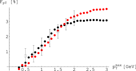
Figure 3: Dependence of $F_{p_{T}}$ on the cut in the transverse momentum. The data points come from Ref. [3]. Red points show the model calculation with $T=165$ MeV, while the black points are for $T=130$ MeV.

A feature of our model is a saturation of $F_{p_{T}}$ at large values of $p_{T}^{\rm max}$. This saturation is a consequence of the thermal model. As a matter of fact, all relevant quantities saturate when integrated over $p_{T}$. Unfortunately, the experimental data do not extend to the saturation region. What is somewhat surprising at the first sight is the rather large value of $p_{T}^{\rm max}$ needed for saturation: about 2 GeV for $T=130$ MeV and about 3 GeV for $T=165$ MeV. Figure 4 shows the results for the average momentum, its variance, and the covariance resulting from the lumped cluster model. We note that all these quantities saturate at rather large values of $p_{T}^{\rm max}$. In that sense in the present context the “soft” thermal physics reaches transverse momenta up to 2-3 GeV!

Figure 4: The dependence of the average momentum (top), its variance (middle), and the covariance (bottom) resulting from the lumped cluster model for $T=130$ MeV (left) and $T=165$ MeV (right) on the cut-off in the transverse momentum, $p_{T}^{\rm max}$.

9 Conclusion

We list our main results:

1. The cluster scaling of $\sigma^{2}_{\rm dyn}$ with $1/{\bar{n}}$ in the fiducial centrality range 0-30% at PHENIX points at the cluster picture of the fireball.

2. Similar scaling can be also seen at STAR [4, 5] (see also Paul Sorensen’s talk) and at CERES [6].

3. Scaling can be found with various correlation measures, which in the limit of sharp distributions and small dynamical compared to statistical fluctuations become equivalent and related in simple ways to the covariance, as discussed in [32].

4. The clusters may a priori originate from very different physics: (mini)jets, droplets of fluid formed in the explosive scenario of the collision, or other mechanisms leading to multiparticle correlations.

5. (Mini)jets just produce clusters, so it is impossible to prove or disprove their existence based solely on the centrality dependence of the correlation data at soft/medium values of $p_{T}$.

6. Resonance decays in a thermal model yield a very small value of the $p_{T}$-covariance.

7. In a model where matter forms lumps moving at similar collective velocity and particles move thermally within a cluster, description of the RHIC data requires on the average 6-15 particles in the cluster. In general, a larger number of particles within a cluster helps to obtain the large (compared to $\sigma_{p}^{2})/{\bar{n}}$) measured value of $\sigma_{\rm dyn}^{2}$.

8. In the “lumped cluster” model the $p_{T}^{\max}$ dependence of $F_{p_{T}}$ grows monotonically and then saturates. It would be interesting to confront this finding to the data.

9. Detailed microscopic modeling would be very useful in order to better understand the problem on transverse momentum correlations in relativistic heavy-ion collisions.

Appendix A Relation of measures of fluctuations to covariance

One difficulty in comparing results of event-by-event momentum fluctuations presented by various experimental groups is the multitude of measures used. Here we briefly show how under assumptions of 1) small dynamical compared to statistical fluctuations and 2) sharp distribution in the multiplicity variable these measures are simply proportional to the covariance. Although these remarks are perhaps obvious to practitioners in the field, they seem worth reminding, as discussions showed confusion.

Suppose we have events of class $n$ (formally, this can be any number chracteristic of the event: the multiplicity of detected particles, the number of participants, the response of a given detector, etc., distributed according to the probability distribution $P_{n}$. Let $\rho_{n}(p_{1},\dots,p_{n})$ denote the $n$-particle distribution of variables $p_{i}$ within events of class $n$, e.g, the distribution of transverse momenta in events of a fixed multiplicity $n$). The subscript _n indicates that $\rho$ depends functionally on $n$. The full probability distribution of obtaining event of class $n$ with momenta $p_{1},\dots,p_{n}$ is

$$P_{n}\rho_{n}(p_{1},\dots,p_{n}).$$ (15)

The marginal probability distributions are obtained from $\rho_{n}(p_{1},\dots,p_{n})$ by integrating over $k$ momenta,

$$\rho_{n}(p_{1},\dots,p_{n-k})=\int dp_{n-k+1}\dots dp_{n}\rho_{n}(p_{1},\dots,p_{n}).$$ (16)

Next, we introduce the relevant moments for the distributions of class $n$:

$$\overline{p_{n}} = \int dp\rho_{n}(p)p,$$

$$\sigma^{2}_{n}(p) = \int dp\rho_{n}(p)(p-\overline{p_{n}})^{2},$$

$${\rm cov}_{n}(p_{1},p_{2}) = \int dp_{1}dp_{2}\rho_{n}(p_{1},p_{2})(p_{1}-\overline{p_{n}})(p_{2}-\overline{p_{n}}),$$ (17)

where $\rho_{n}(p)$ and $\rho_{n}(p_{1},p_{2})$ are the one- and two-particle marginal distributions within the class $n$. Now, in a typical setup we are interested in broader classes, containing $n$ in the range $n_{1}\leq n\leq n_{2}$. We denote for brevity $\sum_{n}=\sum_{n=n_{1}}^{n_{2}}$.

Let us illustrate the basic statistical facts on the example of the measures $\sigma^{2}_{\rm dyn}$ and $F_{p_{T}}$. For other measures the analysis is analogous. Consider the variable $M_{n}=(p_{1}+\dots+p_{n})/n$, i.e. the average value of the variable $p$. Then

$$\overline{M} = \sum_{n}P_{n}\int dp_{1}\dots dp_{n}\rho_{n}(p_{1},\dots,p_{n})\frac{p_{1}+\dots+p_{n}}{n}=\sum_{n}P_{n}\overline{p_{n}},$$

$$\overline{M^{2}} = \sum_{n}P_{n}\int dp_{1}\dots dp_{n}\rho_{n}(p_{1},\dots,p_{n})\frac{1}{n^{2}}\sum_{i,j=1}^{n}\left[(p_{i}-\overline{p_{n}})(p_{j}-\overline{p_{n}})+\overline{p_{n}}^{2}\right],$$

$${\sigma^{2}_{M}} = \overline{M^{2}}-\overline{M}^{2}=\sum_{n}P_{n}\overline{p_{n}}^{2}-\left(\sum_{n}P_{n}\overline{p_{n}}\right)^{2}+\sum_{n}P_{n}\frac{\sigma^{2}_{n}(p)}{n}+\sum_{n}P_{n}\frac{1}{n^{2}}\sum_{i\neq j=1}^{n}{\rm cov}_{n}(p_{i},p_{j}).$$ (18)

Suppose mixing of events is performed. Then, by definition, no correlations are present, i.e., ${\rm cov}^{\rm mix}_{n}(p_{i},p_{j})=0$, and

$${\sigma^{2,{\rm mix}}_{M}}=\sum_{n}P_{n}\overline{p_{n}}^{2}-\left(\sum_{n}P_{n}\overline{p_{n}}\right)^{2}+\sum_{n}P_{n}\frac{\sigma^{2}_{n}(p)}{n}.$$ (19)

By definition, $\sigma^{2}_{\rm dyn}=\sigma^{2}_{M}-{\sigma^{2,{\rm mix}}_{M}}$. With above results

$$\sigma^{2}_{\rm dyn}=\sum_{n}P_{n}\frac{1}{n^{2}}\sum_{i\neq j}{\rm cov}_{n}(p_{i},p_{j}).$$ (20)

Note that all above results are exact, just following from obvious manipulations. Thus $\sigma^{2}_{\rm dyn}$ is a weighted sum of total (summed over particle pairs) covariances at fixed $n$, $\sum_{i\neq j}{\rm cov}_{n}(p_{i},p_{j})$, with weights equal to $P_{n}\frac{1}{n^{2}}$. Moreover, all quantities in Eq.(18) or (19) are possible to obtain experimentally from the given event sample.

Now let us have a look on $F_{p_{T}}\equiv(\sqrt{\omega}-\sqrt{\omega_{\rm mix}})/\sqrt{\omega_{\rm mix}}$, where $\omega=\sigma^{2}_{M}/\overline{M}$. We find immediately

$$F_{p_{T}}=\frac{\sigma_{M}}{\sigma^{{\rm mix}}_{M}}-1=\sqrt{1+\frac{\sigma^{2}_{\rm dyn}}{\sigma^{2,{\rm mix}}_{M}}}-1.$$ (21)

Again, this is an exact relation. At RHIC $\sigma^{2}_{\rm dyn}\ll\sigma^{2,{\rm mix}}_{M}$, hence we can expand

$$F_{p_{T}}\simeq\frac{1}{2}\frac{\sigma^{2}_{\rm dyn}}{\sigma^{2,{\rm mix}}_{M}},$$ (22)

which shows the proportionality of the two measures in the limit of small dynamical correlations.

A further simplification occurs when the distributions $P_{n}$ are sharply peaked around some $\overline{n}$, which again is sufficiently well satisfied at RHIC. Then for a smooth function $f(n)$

$$\sum_{n}\frac{P_{n}}{n^{z}}f(n)\simeq\frac{f(\overline{n})}{\overline{n}^{z}}.$$ (23)

In this sharp limit

$$\sigma^{2}_{\rm dyn} \simeq \frac{1}{\overline{n}^{2}}\sum_{i\neq j}{\rm cov}_{\overline{n}}(p_{i},p_{j}),$$

$$\sigma^{2,{\rm mix}}_{M} \simeq \frac{\sigma^{2}_{\overline{n}}(p)}{\overline{n}}.$$ (24)

For other measures the results are similar. For $\Sigma^{2}_{p_{T}}$ we have from definition $\Sigma^{2}_{p_{T}}\equiv{\sigma^{2}_{\rm dyn}}/{\overline{p}^{2}}$, for $\Phi_{p_{T}}$ under conditions 1) and 2)

$$\Phi_{p_{T}}\equiv\sqrt{\frac{\sigma_{S}^{2}}{\overline{n}}}-\sigma_{\overline{n}}(p)\simeq\frac{\sum_{i\neq j}{\rm cov}_{\overline{n}}}{2\overline{n}\sigma_{\overline{n}}(p)},$$ (25)

where $S_{n}=p_{1}+\dots+p_{n}$.

Conclusion: Since at RHIC conditions 1) and 2) hold, the popular measures of event-by-event fluctuations are proportional to the covariance. Full information on correlations could be acquired by simply evaluating the covariance $\sum_{i\neq j}{\rm cov}_{n}$ for each $n$. If 1) or 2) are relaxed, then, of course, the measures are no longer equivalent, but they are still related to the sum of the weighted covariances at various $n$ in the way dependent on the particular measure.

Finally, we make a digression concerning the inclusive distributions, not used in our derivations but appearing frequently in similar studies. They should not be confused with the marginal distributions, to which they are related as follows:

$$\rho_{\rm in}(p) = \sum_{n}P_{n}\int dp_{1}\dots dp_{n}\sum_{i=1}^{n}\delta(p-p_{i})\rho_{n}(p_{1},\dots,p_{n}),$$

$$\rho_{\rm in}(p,q) = \sum_{n}P_{n}\int dp_{1}\dots dp_{n}\sum_{i\neq j=1}^{n}\delta(p-p_{i})\delta(q-p_{j})\rho_{n}(p_{1},\dots,p_{n}),$$ (26)

with the properties

$$\int dp\rho_{\rm in}(p) = \overline{n},$$

$$\int dpdq\rho_{\rm in}(p,q) = \overline{n(n-1)},$$

$$\overline{p_{\rm in}} = \sum_{n}nP_{n}\overline{p_{n}}.$$ (27)

References

- [1] W. Broniowski, B. Hiller, W. Florkowski and P. Bozek, Phys. Lett. B 635 (2006) 290, nucl-th/0510033.
- [2] PHENIX, K. Adcox et al., Phys. Rev. C66 (2002) 024901, nucl-ex/0203015.
- [3] PHENIX, S.S. Adler et al., Phys. Rev. Lett. 93 (2004) 092301, nucl-ex/0310005.
- [4] STAR, J. Adams et al., Phys. Rev. C71 (2005) 064906, nucl-ex/0308033.
- [5] J. Adams et al. [STAR Collaboration], Phys. Rev. C 72 (2005) 044902, arXiv:nucl-ex/0504031.
- [6] H. Appelshaeuser et al., Nucl. Phys. A752 (2005) 394.
- [7] See these proceedings.
- [8] Proceedings of workshop on CORRELATIONS AND FLUCTUATIONS IN RELATIVISTIC NUCLEAR COLLISIONS, 21-23 April 2005, Massachusetts Institute of Technology, Boston, USA J. Phys.: Conference Series 27 (2005).
- [9] M. Gazdzicki and S. Mrowczynski, Z. Phys. C54 (1992) 127.
- [10] L. Stodolsky, Phys. Rev. Lett. 75 (1995) 1044.
- [11] E.V. Shuryak, Phys. Lett. B423 (1998) 9, hep-ph/9704456.
- [12] S. Mrowczynski, Phys. Lett. B430 (1998) 9, nucl-th/9712030.
- [13] M.A. Stephanov, K. Rajagopal and E.V. Shuryak, Phys. Rev. D60 (1999) 114028, hep-ph/9903292.
- [14] S.A. Voloshin, V. Koch and H.G. Ritter, Phys. Rev. C60 (1999) 024901, nucl-th/9903060.
- [15] NA49, H. Appelshauser et al., Phys. Lett. B459 (1999) 679, hep-ex/9904014.
- [16] O. V. Utyuzh, G. Wilk and Z. Wlodarczyk, J. Phys. G 26, L39 (2000) [arXiv:hep-ph/9906500].
- [17] R. Korus et al., Phys. Rev. C64 (2001) 054908, nucl-th/0106041.
- [18] G. Baym and H. Heiselberg, Phys. Lett. B469 (1999) 7, nucl-th/9905022.
- [19] A. Bialas and V. Koch, Phys. Lett. B456 (1999) 1, nucl-th/9902063.
- [20] E. G. Ferreiro, F. del Moral, and C. Pajares, Phys. Rev. C69 (2004) 034901.
- [21] L. Cunqueiro, E. G. Ferreiro, F. del Moral, and C. Pajares, Phys. Rev. C72 (2005) 024907.
- [22] P. Brogueira and J. Dias de Deus, Acta Phys. Pol. B36 (2005) 307.
- [23] M. Asakawa, U.W. Heinz and B. Muller, Phys. Rev. Lett. 85 (2000) 2072, hep-ph/0003169.
- [24] H. Heiselberg, Phys. Rept. 351 (2001) 161, nucl-th/0003046.
- [25] O. V. Utyuzh, G. Wilk and Z. Wlodarczyk, Phys. Rev. C 64, 027901 (2001) [arXiv:hep-ph/0103158].
- [26] C. Pruneau, S. Gavin and S. Voloshin, Phys. Rev. C66 (2002) 044904, nucl-ex/0204011.
- [27] S. Jeon and V. Koch, in Quark-Gluon Plasma 3, eds. R. C. Hwa and X. N. Wang, p. 430, World Scientific Singapore (2004), hep-ph/0304012.
- [28] S. Gavin, Phys. Rev. Lett. 92 (2004) 162301, nucl-th/0308067.
- [29] M. Abdel-Aziz and S. Gavin, Nucl. Phys. A 774, 623 (2006) [arXiv:nucl-th/0510011].
- [30] M. Abdel-Aziz and S. Gavin, Int. J. Mod. Phys. A 20 (2005) 3786.
- [31] Q.J. Liu and T.A. Trainor, Phys. Lett. B567 (2003) 184, hep-ph/0301214.
- [32] W. Broniowski, contribution “Round Table Discussion: Correlations and Fluctuations in Nuclear Collisions” in these proceedings (here included as Appendix A).
- [33] J. T. Mitchell, J. Phys. Conf. Ser. 27 (2005) 88, arXiv:nucl-ex/0511033.
- [34] W. Broniowski and W. Florkowski, Phys. Rev. Lett. 87 (2001) 272302, nucl-th/0106050.
- [35] W. Broniowski, A. Baran and W. Florkowski, Acta Phys. Polon. B33 (2002) 4235, hep-ph/0209286.
- [36] P. Bozek, W. Broniowski and W. Florkowski, Acta Phys. Hung. A22 (2005) 149, nucl-th/0310062.
- [37] A. Kisiel, T. Taluc, W. Broniowski and W. Florkowski, Comput. Phys. Commun. 174 (2006) 669, arXiv:nucl-th/0504047.
- [38] S. Cheng et al., Phys. Rev. C69 (2004) 054906, nucl-th/0401008.