Overview of Non-Relativistic QCD

Abstract

An overview of recent theoretical progress on Non-Relativistic QCD and related effective theories is provided.

1 Introduction

Heavy quarkonium systems have been a good laboratory to test our theoretical ideas since the early days of QCD (see Brambilla:2004wf for an extensive review). Based on the pioneering work of Caswell and Lepage Caswell:1985ui , a systematic approach to study such systems from QCD has been developed over the years which makes use of effective field theory techniques and is generically known as Non-Relativistic QCD (NRQCD) Bodwin:1994jh . NRQCD has been applied to spectroscopy, decay and production of heavy quarkonium. The NRQCD formalism for spectroscopy and decay is very well understood (this is also so for electromagnetic threshold production) so that NRQCD results may be considered QCD results up to a given order in the expansion parameters (usually $\alpha_{\rm s}(m_{Q})$ and $1/m_{Q}$, $m_{Q}$ being the heavy quark mass). I will restrict myself to review recent progress on these issues and refer the reader to the review Brambilla:2004jw for earlier developments. The NRQCD formalism for production is more controversial. Important work has been carried out recently to which I will devote some time.

2 Heavy Quarkonium

Heavy quarkonia are mesons made out of a heavy quark and a heavy antiquark (not necessarily of the same flavor), whose masses are larger than $\Lambda_{QCD}$, the typical hadronic scale. These include bottomonia ($b\bar{b}$), charmonia ($c\bar{c}$), $B_{c}$ systems ($b\bar{c}$ and $c\bar{b}$) and would-be toponia ($t\bar{t}$). Baryons made out of two or three heavy quarks share some similarities with these systems (see Brambilla:2005yk ; Fleming:2005pd ).

In the quarkonium rest frame the heavy quarks move slowly ($v\ll 1$, $v$ being the typical heavy quark velocity in the center of mass frame), with a typical momentum $m_{Q}v\ll m_{Q}$ and binding energy $\sim m_{Q}v^{2}$. Hence any study of heavy quarkonium faces a multiscale problem with the hierarchies $m_{Q}\gg m_{Q}v\gg m_{Q}v^{2}$ and $m_{Q}\gg\Lambda_{QCD}$. The use of effective field theories is extremely convenient in order to exploit these hierarchies.

3 Effective Field Theories

Direct QCD calculations in multiscale problems are extremely difficult, no matter if one uses analytic approaches (i.e. perturbation theory) or numerical ones (i.e. lattice). We may try to construct a simpler theory (the effective field theory (EFT)), in which less scales are involved in the dynamics and which is equivalent to the fundamental theory (QCD) in the particular energy region where heavy quarkonia states lie. The clues for the construction are: (i) identify the relevant degrees of freedom, (ii) enforce the QCD symmetries and (iii) exploit the hierarchy of scales. Typically one integrates out the higher energy scales so that the lagrangian of the EFT can be organized as a series of operators over powers of these scales. Each operator has a so called matching coefficient in front, which encodes the remaining information on the higher energy scales. The matching coefficients may be calculated by imposing that a selected set of observables coincide when are calculated in the fundamental and in the effective theory.

NRQCD is the (first) effective theory relevant for heavy quarkonium. Out of the four components of the relativistic Dirac fields describing the heavy quarks (antiquarks) only the upper (lower) are relevant for energies lower than $m_{Q}$ (no pair production is allowed anymore). Hence a two component Pauli spinor field is used to describe the quark (antiquark). The hierarchy of scales exploited in NRQCD is $m_{Q}\gg m_{Q}v,m_{Q}v^{2},\Lambda_{QCD}$. The remaining hierarchy $m_{Q}v\gg m_{Q}v^{2}$, may be exploited using a further effective theory called Potential NRQCD (pNRQCD) Pineda:1997bj ; Brambilla:1999xf .

3.1 Non-Relativistic QCD

The part of the NRQCD lagrangian bilinear on the heavy quark fields coincides with the one of Heavy Quark Effective Theory (HQET) (see Neubert:1993mb for a review), and reads

$${\cal L}_{\psi}=\psi^{\dagger}\Biggl{\{}iD_{0}+{1\over 2m_{Q}}{\bf D}^{2}+{1\over 8m_{Q}^{3}}{\bf D}^{4}+{c_{F}\over 2m_{Q}}{\mbox{\boldmath$\sigma$}.g{\bf B}}\,+$$

$$+{c_{D}\over 8m_{Q}^{2}}\left({\bf D}.g{\bf E}-g{\bf E}.{\bf D}\right)+i\,{c_{S}\over 8m_{Q}^{2}}{\mbox{\boldmath$\sigma$}.\left({\bf D}\times g{\bf E}-g{\bf E}\times{\bf D}\right)}\Biggr{\}}\psi$$ (1)

$\psi$ is a Pauli spinor which annihilates heavy quarks. $c_{F}$, $c_{D}$ and $c_{S}$ are short distance matching coefficients which depend on $m_{Q}$ and $\mu$ (factorization scale). Analogous terms exist for $\chi$, a Pauli spinor field which creates antiquarks. Unlike HQET, it also contains four fermion operators,

$${\cal L}_{\psi\chi} = {f_{1}(^{1}S_{0})\over m_{Q}^{2}}O_{1}(^{1}S_{0})+{f_{1}(^{3}S_{1})\over m_{Q}^{2}}O_{1}(^{3}S_{1})+$$

$$+{f_{8}(^{1}S_{0})\over m_{Q}^{2}}O_{8}(^{1}S_{0})+{f_{8}(^{3}S_{1})\over m_{Q}^{2}}O_{8}(^{3}S_{1}),$$

$$O_{1}(^{1}S_{0}) =\psi^{{\dagger}}\chi\,\chi^{{\dagger}}\psi ,\quad O_{1}(^{3}S_{1})=\psi^{{\dagger}}{\mbox{\boldmath$\sigma$}}\chi\,\chi^{{\dagger}}{\mbox{\boldmath$\sigma$}}\psi,$$ (2)

$$O_{8}(^{1}S_{0}) =\psi^{{\dagger}}{\rm T}^{a}\chi\,\chi^{{\dagger}}{\rm T}^{a}\psi ,\quad O_{8}(^{3}S_{1})=\psi^{{\dagger}}{\rm T}^{a}{\mbox{\boldmath$\sigma$}}\chi\,\chi^{{\dagger}}{\rm T}^{a}{\mbox{\boldmath$\sigma$}}\psi.$$

The $f$s are again short distance matching coefficients which depend on $m_{Q}$ and $\mu$, which have imaginary parts when the quark and the antiquark are of the same flavor. This is due to the fact that hard gluons (of energy $\sim m_{Q}$), which remain accessible through annihilation of the quark and antiquark, have been integrated out. The fact that NRQCD is equivalent to QCD at any desired order in $1/m_{Q}$ and $\alpha_{\rm s}(m_{Q})$ makes the lack of unitarity innocuous. In fact, it is turned into an advantage: it facilitates the calculation of inclusive decay rates to light particles.

The lagrangian above can be used as such for spectroscopy, inclusive decays and electromagnetic threshold production of heavy quarkonia. Spectroscopy studies have been carried out on the lattice and are discussed in Vairo:2006nq (see also Gray:2005ur and references therein).

3.1.1 Inclusive decays

Let us just show, as an example, the NRQCD formula for inclusive decays of P-wave states to light hadrons at leading order

$$\Gamma(\chi_{Q}(nJS)\rightarrow LH)={2\over m_{Q}^{2}}\Bigg{(}{\rm Im\,}f_{1}(^{2S+1}P_{J})\times$$

$$\times{\langle\chi_{Q}(nJS)|O_{1}(^{2S+1}P_{J})|\chi_{Q}(nJS)\rangle\over m_{Q}^{2}}$$

$$+{\rm Im\,}f_{8}(^{2S+1}S_{S})\langle\chi_{Q}(nJS)|O_{8}(^{1}S_{0})|\chi_{Q}(nJS)\rangle\Bigg{)},$$

$f_{1}$ and $f_{8}$ are short distance matching coefficients which can be calculated in perturbation theory in $\alpha_{\rm s}(m_{Q})$. $O_{1}$ $(^{2S+1}P_{J})$ is a color singlet dimension 8 operator and $O_{8}(^{1}S_{0})$ is the color octet operator given in (2). Earlier QCD factorization formulas were missing the color octet contribution. They are inconsistent because the color octet matrix element is necessary to cancel the factorization scale dependence which arises in one loop calculations of ${\rm Im\,}f_{1}$ $(^{2S+1}P_{J})$ Bodwin:1992ye . The matrix elements cannot be calculated in perturbation theory of $\alpha_{\rm s}(m_{Q})$. They can however be calculated on the lattice (see for instance Bodwin:2001mk ) or extracted from data. The imaginary parts of the matching coefficients of the dimension 6 and 8 operators are known at NLO Petrelli:1997ge , and those of the electromagnetic decays of dimension 10 at LO Brambilla:2006ph ; Bodwin:2002hg ; Ma:2002ev .

3.1.2 Problems

Unlike HQET, in which each term in the lagrangian (2) has a definite size (by assigning $\Lambda_{QCD}^{n}$ to any operator of dimension $n$), NRQCD does not enjoy a homogeneous counting. This is due to the fact that the scales $m_{Q}v$, $m_{Q}v^{2}$ and $\Lambda_{QCD}$ are still entangled. Even though a counting was put forward in Bodwin:1994jh , the so called NRQCD velocity counting, which has become the standard bookkeeping for NRQCD calculations, there is no guarantee that it holds for all the states, and hence there is a problem on how to make a sensible organization of the calculation for a given state. There are two approaches which aim at disentangling these scales, and hence to facilitate the counting. The first one consist of constructing a further effective theory by integrating out energy scales larger $m_{Q}v^{2}$. This is the pNRQCD approach first proposed in Pineda:1997bj , which will be described in the next section. The second one consist in decomposing the NRQCD fields in several modes so that each one has a homogeneous counting. This is the vNRQCD approach first proposed in Luke:1999kz (see also Griesshammer:1997wz ). The scale $\Lambda_{QCD}$ has not been discussed so far in this approach, and, in fact, a consistent formulation has only become available recently Manohar:2006nz (see also Hoang:2002yy ; Manohar ).

3.2 Potential NRQCD

As mentioned above, pNRQCD is the effective theory which arises from NRQCD after integrating out energy scales largen than $m_{Q}v^{2}$, namely than the typical binding energy. If $\Lambda_{QCD}\lesssim m_{Q}v^{2}$, then $m_{Q}v\gg\Lambda_{QCD}$ and the matching between NRQCD and pNRQCD can be carried out in perturbation theory in $\alpha_{\rm s}(m_{Q}v)$ . This is the so called weak coupling regime. If $\Lambda_{QCD}\gg m_{Q}v^{2}$, the matching cannot be carried out in perturbation theory in $\alpha_{\rm s}(m_{Q}v)$ anymore, but one can still exploit the hierarchy $m_{Q}\gg m_{Q}v,\Lambda_{QCD}\gg m_{Q}v^{2}$. This is the so called strong coupling regime.

3.2.1 Weak Coupling Regime

The lagrangian in this regime reads

$$\!\!\!\!\!\!\!{\cal L}_{\rm pNRQCD}=\int d^{3}{\bf r}\;{\rm Tr}\,\Biggl{\{}{\rm S}^{\dagger}\left(i\partial_{0}-h_{s}({\bf r},{\bf p},{\bf P}_{\bf R},{\bf S}_{1},{\bf S}_{2},\mu)\right){\rm S}+$$

$$\qquad\qquad+{\rm O}^{\dagger}\left(iD_{0}-h_{o}({\bf r},{\bf p},{\bf P}_{\bf R},{\bf S}_{1},{\bf S}_{2},\mu)\right){\rm O}\Biggr{\}}$$

$$\qquad\qquad+V_{A}(r,\mu){\rm Tr}\left\{{\rm O}^{\dagger}{\bf r}\cdot g{\bf E}\,{\rm S}+{\rm S}^{\dagger}{\bf r}\cdot g{\bf E}\,{\rm O}\right\}+$$

$$\qquad\qquad+{V_{B}(r,\mu)\over 2}{\rm Tr}\left\{{\rm O}^{\dagger}{\bf r}\cdot g{\bf E}\,{\rm O}+{\rm O}^{\dagger}{\rm O}{\bf r}\cdot g{\bf E}\right\}$$

where $S$ and $O$ are color singlet and color octet wave function fields respectively. $h_{s}$ and $h_{o}$ are color singlet and color octet hamiltonians respectively, which may be obtained by matching to NRQCD in perturbation theory in $\alpha_{\rm s}(m_{Q}v)$ and $1/m_{Q}$ at any order of the multipole expansion (${\bf r}\sim 1/m_{Q}v$). The static potential terms in $h_{s}$ and $h_{o}$ are known at two loops Peter:1997me ; Schroder:1998vy ; Kniehl:2004rk (the logarithmic contributions at three loops and (for $h_{s}$ only) at four loops are also known Brambilla:1999qa ; Brambilla:1999xf ; Brambilla:2006wp ). The renormalon singularities in the static potentials are also understood in some detail Pineda:2002se ; Bali:2003jq . The $1/m_{Q}$ and $1/m_{Q}^{2}$ terms in $h_{s}$ are known at two and one loop respectively Kniehl:2002br . $V_{A},V_{B}=1+{\cal O}(\alpha_{\rm s}^{2})$ Brambilla:2006wp . This lagrangian has been used to carry our calculations at fixed order in $\alpha_{\rm s}$: an almost complete NNNLO (assuming $\Lambda_{QCD}\ll m_{Q}\alpha_{\rm s}^{2}$) expression for the spectrum is available Penin:2002zv . Most remarkably resummations of logarithms can also be carried out using renormalization group techniques Pineda:2001ra ; Pineda:2001et ; Pineda:2002bv . Thus the $\eta_{b}$ mass and its electromagnetic decay width have been predicted at NNLL and NLL respectively Kniehl:2003ap ; Penin:2004ay .

3.2.2 Strong Coupling Regime

The lagrangian in this regime reads

$$L_{\rm pNRQCD}=\int d^{3}{\bf R}\int d^{3}{\bf r}\;S^{\dagger}\big{(}i\partial_{0}-h_{s}({\bf r},{\bf p},{\bf P_{R}},{\bf S}_{1},{\bf S}_{2})\big{)}S,$$

$$h_{s}({\bf r},{\bf p},{\bf P_{R}},{\bf S}_{1},{\bf S}_{2})={{\bf p}^{2}\over m_{Q}}+{{\bf P_{R}}_{2}^{2}\over 4m_{Q}}+V_{s}({\bf r},{\bf p},{\bf P_{R}},{\bf S}_{1},{\bf S}_{2}),$$

$$V_{s}=V^{(0)}_{s}+{V^{(1)}_{s}\over m_{Q}}+{V^{(2)}_{s}\over m_{Q}^{2}}+\cdots,$$

$V_{s}$ cannot be calculated in perturbation theory of $\alpha_{\rm s}(m_{Q}v)$ anymore, but can indeed be, and most of the terms have been, calculated on (quenched) lattice simulations Koma ; Bali:1997am ; Necco:2001xg ; Koma:2006si ; Koma:2006fw (see Jugeau:2003df for a large $N_{c}$ calculation). The fact that $\Lambda_{QCD}\gg m_{Q}v^{2}$ can now be exploited to further factorize NRQCD matrix elements Brambilla:2001xy ; Brambilla:2002nu ; Brambilla:2003mu , for instance

$$\langle\Upsilon(n)|O_{8}(^{1}S_{0})|\Upsilon(n)\rangle=C_{A}{|R_{n}({0})|^{2}\over 2\pi}\left(-{(C_{A}/2-C_{f})c_{F}^{2}{\cal B}_{1}\over 3m_{Q}^{2}}\right)$$

were $R_{n}({0})$ is the wave function at the origin, ${\cal B}_{1}\sim\Lambda_{QCD}^{2}$ is a universal (independent of $n$) non-perturbative parameter, and $c_{F}$ a (computable) short distance matching coefficient. This further factorization allows to put forward new model independent predictions, for instance the ratios of hadronic decay widths of P-wave states in bottomonium were predicted from charmonium data Brambilla:2001xy , or the ratio of photon spectra in radiative decays of vector resonances GarciaiTormo:2005bs , as we will see below.

3.2.3 Weak or Strong (or else)?

Since $m_{Q}$ , $v$ and $\Lambda_{QCD}$ are not directly observable, given heavy quarkonium state it is not clear to which of the above regimes, if to any , it must be assigned to. The leading non-perturbative ($\sim\Lambda_{QCD}$) corrections to the spectrum in the weak coupling regime scale as a large power of the principal quantum number Voloshin:1978hc ; Leutwyler:1980tn , which suggests that only the $n=1$ states of bottomonium and charmonium may belong to this regime. However if one ignores this and proceeds with weak coupling calculations one finds, for instance, that renormalon based approaches at NNLO Brambilla:2001fw ; Brambilla:2001qk and the NNNLO calculation Penin:2004ay give a reasonable description of the bottomonium spectrum up to $n=3$. It has recently been proposed that precise measurements of the photon spectra in radiative decays, as the ones carried out by CLEO Besson:2005jv , will clarify the assignments GarciaiTormo:2005bs . It turns out that in the strong coupling regime one can work out the following formula, which holds at NLO,

$$\frac{\displaystyle\frac{d\Gamma_{n}}{dz}}{\displaystyle\frac{d\Gamma_{r}}{dz}}=\frac{\langle\mathcal{O}_{1}(^{3}S_{1})\rangle_{n}}{\langle\mathcal{O}_{1}(^{3}S_{1})\rangle_{r}}\left(1+\frac{C_{1}^{\prime}\left[\phantom{}{}^{3}S_{1}\right](z)}{C_{1}\left[\phantom{}{}^{3}S_{1}\right](z)}\frac{1}{m_{Q}}\left(E_{n}-E_{r}\right)\right)$$

$$\frac{\langle\mathcal{O}_{1}(^{3}S_{1})\rangle_{n}}{\langle\mathcal{O}_{1}(^{3}S_{1})\rangle_{r}}=\frac{\Gamma\left(\Upsilon(n)\to e^{+}e^{-}\right)}{\Gamma\left(\Upsilon(r)\to e^{+}e^{-}\right)}\left[\!1\!-\!\frac{\mathrm{Im}g_{ee}\left(\phantom{}{}^{3}S_{1}\right)}{\mathrm{Im}f_{ee}\left(\phantom{}{}^{3}S_{1}\right)}\frac{E_{n}-E_{r}}{m_{Q}}\right]$$

$C_{1}^{\prime}\left[\phantom{}{}^{3}S_{1}\right](z)$, $C_{1}\left[\phantom{}{}^{3}S_{1}\right](z)$, $\mathrm{Im}g_{ee}\left(\phantom{}{}^{3}S_{1}\right)$, $\mathrm{Im}f_{ee}\left(\phantom{}{}^{3}S_{1}\right)$ are matching coefficients computable in perturbation theory, and $E_{n}-E_{r}$ the mass difference between the two states. If data follow this formula it will indicate that both $n$ and $r$ are in the strong coupling regime. For the $n=1,2,3$ of bottomonia, current data disfavor $n=1$ in the strong coupling regime and is compatible with $n=2,3$ in it.

3.3 Soft-Collinear Effective Theory

For exclusive decays and for certain kinematical end-points of semi-inclusive decays, NRQCD must be supplemented with collinear degrees of freedom. This can be done in the effective theory framework of Soft-Collinear Effective Theory (SCET)Bauer:2000ew ; Bauer:2000yr . Exclusive radiative decays of heavy quarkonium in SCET have been addressed in Fleming:2004hc , where results analogous to those of traditional light cone factorization formulas have been obtained Ma:2001tt . Concerning semi-inclusive decays, let me focus on the photon spectrum of $\Upsilon(1S)\rightarrow\gamma X$ when the photon is very energetic. Describing experimental data in this region has been a challenge since the early days of QCD, and the best fits were obtained using a model with a finite gluon mass of the order of the GeV. Field:2001iu . The naive inclusion of color octet contributions in the NRQCD framework seemed to further deepen the discrepancy Wolf:2000pm . In recent years a remarkable improvement in the understanding of this end-point region has been achieved by combining SCET and NRQCD. The following factorization formula has been proved Fleming:2002rv ; Fleming:2002sr

$$\frac{d\Gamma^{e}}{dz}=\sum_{\omega}H(M,\omega,\mu)\int dkS(k,\mu)\mathrm{Im}J_{\omega}(k+M(1-z),\mu)$$

where $H$ is a hard matching coefficient computable in perturbation theory, $J_{w}$ is a jet function (also computable in perturbation theory if z is not too close to $1$) and $S$ is a (soft) shape function which depends on the bound state dynamics. $M$ is the heavy quarkonium mass and $\mu$ a factorization scale. Large (Sudakov) logs have been resummed using renormalization group equations both in the color octet Bauer:2001rh and color singlet Fleming:2004rk contributions. Furthermore, using pNRQCD the shape function $S$ has been calculated GarciaiTormo:2004jw . When all this is put together an excellent description of data is achieved GarciaiTormo:2005ch , see Fig. 1.

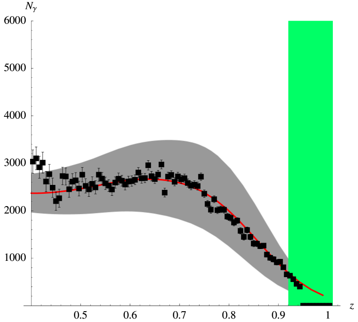
Figure 1: $N_{\gamma}$ is the number of photons and $z$ the energy of the photons normalized to half the $\Upsilon(1S)$ mass. The black squares are CLEO data Besson:2005jv and the (red) solid curve the theoretical result of GarciaiTormo:2005ch with theoretical errors (grey band) displayed. The (green) rectangle on the right displays the region where the theoretical results are not reliable. The plot is taken from Tormo:2006ew .

4 Production

Production of heavy quarkonium is a far more complicated issue than spectroscopy and decay. This is due to the fact that in addition to the several scales which characterize the heavy quarkonium system, further scales due to the kinematics of the production process may also appear.

4.1 Electromagnetic threshold production

This is the simplest and best understood production process in the weak coupling regime, which is relevant for a precise measurement of top quark mass in the future International Linear Collider. The cross-section at NNLO is known for some time Hoang:2000yr and the log resummation at NLL is also available Pineda:2001et ; Hoang:2002yy . The effort is now in calculations at NNNLO, where partial results already exist Kniehl:1999mx ; Hoang:2003ns ; Kniehl:2002yv ; Beneke:2005hg ; Penin:2005eu ; Marquard:2006qi , and in the log resummation at NNLL, where partial results also exist Hoang:2003ns ; Pineda:2006ri . At this level of precision electroweak effect must also be taken into account Hoang:2004tg ; Hoang:2006pd ; Eiras:2006xm (see Hoang:2006pc ; Signer:2006vq for recent reviews).

4.2 Inclusive production

A factorization formula for the inclusive production of heavy quarkonium was put forward in Bodwin:1994jh , which was assumed to hold provided that the tranverse momentum ${\bf p_{\perp}}$ was larger or of the order of the heavy quark mass,

$$\sigma(H)\;=\;\sum_{n}{F_{n}(\mu)\over m_{Q}^{d_{n}-4}}\;{\langle 0|}{\cal O}^{H}_{n}(\mu){|0\rangle},$$

The formula contains a partonic level cross section ($F_{n}(\mu)/$ $m_{Q}^{d_{n}-4}$) in which the heavy quark pair may be produced in color singlet or a color octet state, and long distance production matrix elements (${\langle 0|}{\cal O}^{H}_{n}(\mu){|0\rangle}$) which encode the evolution of the pair to the actual physical state. The production matrix elements have the generic form

$${\cal O}^{H}_{n} = \chi^{\dagger}{\cal K}_{n}\psi\left(\sum_{X}\sum_{m_{J}}{|H+X\rangle}{\langle H+X|}\right)\psi^{\dagger}{\cal K}_{n}^{\prime}\chi$$

where the sums are over the $2J+1$ spin states of the quarkonium $H$ and over all other final-state particles $X$. ${\cal K}_{n}$, ${\cal K}_{n}^{\prime}$ are gluonic operators (including no gluon content and covariant derivatives). The production matrix elements were assigned sizes according to the velocity scaling rules of Bodwin:1994jh , which, as discussed above, correspond to the weak coupling regime. A great success of this formula was the explanation of charmonium production a the Tevatron Braaten:1994vv , and it has been applied to a large number of production processes (see Kramer:2001hh ; Bodwin:2003kc ; Bodwin:2005ec for reviews), including some NLO calculations in photoproduction Klasen:2004tz ; Klasen:2004az . This factorization formalism has received a closer look recently in the framework of fragmentation functions, and has been proved to be correct at NNLO in $\alpha_{\rm s}(m_{Q})$, provided a slight redefinition of the matrix elements is carried out Nayak:2005rw ; Nayak:2005rt ; Nayak:2006fm . The interplay of the scales $m_{Q}v$, $m_{Q}v^{2}$ and $\Lambda_{QCD}$ has not been discussed in detail for production. This may be important in resolving the polarization puzzle at the Tevatron Affolder:2000nn , since the NRQCD prediction that heavy quarkonium must be produced transversely polarized in fragmentation processes Cho:1994ih , sometimes phrased as a smoking gun for NRQCD, depends crucially on the velocity counting used. For instance, in the strong coupling regime one would not expect a sizable polarization Fleming:2000ib .

Near certain kinematical end-points NRQCD production processes must be supplemented with collinear degrees of freedom, in analogy to semi-inclusive decays discussed above. This issue has recently been addressed using SCET Fleming:2003gt ; Hagiwara:2004pf ; Lin:2004eu ; Fleming:2006cd .

4.3 Exclusive production

Although no detailed formalism has been worked out for exclusive production, the basic ideas of NRQCD factorization have indeed been applied to it Braaten:2002fi ; Zhang:2005ch , mostly after the surprisingly large double charmonium cross-section first measured at Belle Abe:2002rb . The traditional light-cone factorization does not seem to have major problems to accommodate this cross-section Ma:2004qf ; Bondar:2004sv ; Braguta:2006py , although some modeling of the light-cone distribution amplitudes has so far been required. Recently, a further factorization of these objects in NRQCD has been presented Ma:2006hc , and a detailed comparison of the NRQCD and light-cone approaches has been carried out Bodwin:2006dm (see also Braguta:2006wr ). The latter suggests that the actual cross-section may well be accommodated into the NRQCD factorization results once higher order contributions in the velocity expansion are taken into account.

5 Conclusions

The NRQCD formalism provides a solid QCD-based framework where heavy quarkonium spectroscopy and inclusive decays can be systematically described starting from QCD. An NRQCD factorization formalism has also been put forward for semi-inclusive decays, inclusive production and, more recently, exclusive production, which, in spite of its successes, is not so well understood theoretically. Nevertheless, remarkable progress has been done recently concerning the structure of the factorization formulas for inclusive processes and the relation to the light-cone formalism for exclusive ones. Certain kinematical end-points both in semi-inclusive decays and production require the inclusion of collinear degrees of freedom in NRQCD. Progress has also occurred here by combining NRQCD and SCET.

References

- (1) N. Brambilla et al., arXiv:hep-ph/0412158.
- (2) W. E. Caswell and G. P. Lepage, Phys. Lett. B 167 (1986) 437.
- (3) G. T. Bodwin, E. Braaten and G. P. Lepage, Phys. Rev. D 51 (1995) 1125 [Erratum-ibid. D 55 (1997) 5853] [arXiv:hep-ph/9407339].
- (4) N. Brambilla, A. Pineda, J. Soto and A. Vairo, Rev. Mod. Phys. 77 (2005) 1423 [arXiv:hep-ph/0410047].
- (5) N. Brambilla, A. Vairo and T. Rosch, Phys. Rev. D 72 (2005) 034021 [arXiv:hep-ph/0506065].
- (6) S. Fleming and T. Mehen, Phys. Rev. D 73 (2006) 034502 [arXiv:hep-ph/0509313].
- (7) A. Pineda and J. Soto, Nucl. Phys. Proc. Suppl. 64 (1998) 428 [arXiv:hep-ph/9707481].
- (8) N. Brambilla, A. Pineda, J. Soto and A. Vairo, Nucl. Phys. B 566 (2000) 275 [arXiv:hep-ph/9907240].
- (9) M. Neubert, Phys. Rept. 245 (1994) 259 [arXiv:hep-ph/9306320].
- (10) A. Vairo, these proceedings, arXiv:hep-ph/0610251.
- (11) A. Gray, I. Allison, C. T. H. Davies, E. Dalgic, G. P. Lepage, J. Shigemitsu and M. Wingate, Phys. Rev. D 72 (2005) 094507 [arXiv:hep-lat/0507013].
- (12) G. T. Bodwin, E. Braaten and G. P. Lepage, Phys. Rev. D 46 (1992) 1914 [arXiv:hep-lat/9205006].
- (13) G. T. Bodwin, D. K. Sinclair and S. Kim, Phys. Rev. D 65 (2002) 054504 [arXiv:hep-lat/0107011].
- (14) A. Petrelli, M. Cacciari, M. Greco, F. Maltoni and M. L. Mangano, Nucl. Phys. B 514 (1998) 245 [arXiv:hep-ph/9707223].
- (15) N. Brambilla, E. Mereghetti and A. Vairo, JHEP 0608 (2006) 039 [arXiv:hep-ph/0604190].
- (16) G. T. Bodwin and A. Petrelli, Phys. Rev. D 66 (2002) 094011 [arXiv:hep-ph/0205210].
- (17) J. P. Ma and Q. Wang, Phys. Lett. B 537, 233 (2002) [arXiv:hep-ph/0203082].
- (18) M. E. Luke, A. V. Manohar and I. Z. Rothstein, Phys. Rev. D 61 (2000) 074025 [arXiv:hep-ph/9910209].
- (19) H. W. Griesshammer, Phys. Rev. D 58 (1998) 094027 [arXiv:hep-ph/9712467].
- (20) A. V. Manohar and I. W. Stewart, arXiv:hep-ph/0605001.
- (21) A. H. Hoang and I. W. Stewart, Phys. Rev. D 67 (2003) 114020 [arXiv:hep-ph/0209340].
- (22) A. Manohar, these proceedings.
- (23) M. Peter, Nucl. Phys. B 501 (1997) 471 [arXiv:hep-ph/9702245].
- (24) Y. Schroder, Phys. Lett. B 447 (1999) 321 [arXiv:hep-ph/9812205].
- (25) B. A. Kniehl, A. A. Penin, Y. Schroder, V. A. Smirnov and M. Steinhauser, Phys. Lett. B 607 (2005) 96 [arXiv:hep-ph/0412083].
- (26) N. Brambilla, A. Pineda, J. Soto and A. Vairo, Phys. Rev. D 60 (1999) 091502 [arXiv:hep-ph/9903355].
- (27) N. Brambilla, X. Garcia i Tormo, J. Soto and A. Vairo, arXiv:hep-ph/0610143.
- (28) A. Pineda, J. Phys. G 29 (2003) 371 [arXiv:hep-ph/0208031].
- (29) G. S. Bali and A. Pineda, Phys. Rev. D 69 (2004) 094001 [arXiv:hep-ph/0310130].
- (30) B. A. Kniehl, A. A. Penin, V. A. Smirnov and M. Steinhauser, Nucl. Phys. B 635 (2002) 357 [arXiv:hep-ph/0203166].
- (31) A. A. Penin and M. Steinhauser, Phys. Lett. B 538 (2002) 335 [arXiv:hep-ph/0204290].
- (32) A. Pineda, Phys. Rev. D 65 (2002) 074007 [arXiv:hep-ph/0109117].
- (33) A. Pineda, Phys. Rev. D 66 (2002) 054022 [arXiv:hep-ph/0110216].
- (34) A. Pineda, Phys. Rev. A 66 (2002) 062108 [arXiv:hep-ph/0204213].
- (35) B. A. Kniehl, A. A. Penin, A. Pineda, V. A. Smirnov and M. Steinhauser, Phys. Rev. Lett. 92 (2004) 242001 [arXiv:hep-ph/0312086].
- (36) A. A. Penin, A. Pineda, V. A. Smirnov and M. Steinhauser, Nucl. Phys. B 699 (2004) 183 [arXiv:hep-ph/0406175].
- (37) Y. Koma, these proceedings.
- (38) G. S. Bali, K. Schilling and A. Wachter, Phys. Rev. D 56 (1997) 2566 [arXiv:hep-lat/9703019].
- (39) S. Necco and R. Sommer, Nucl. Phys. B 622 (2002) 328 [arXiv:hep-lat/0108008].
- (40) Y. Koma, M. Koma and H. Wittig, Phys. Rev. Lett. 97, 122003 (2006) [arXiv:hep-lat/0607009].
- (41) Y. Koma and M. Koma, arXiv:hep-lat/0609078.
- (42) F. Jugeau and H. Sazdjian, Nucl. Phys. B 670 (2003) 221.
- (43) N. Brambilla, D. Eiras, A. Pineda, J. Soto and A. Vairo, Phys. Rev. Lett. 88 (2002) 012003 [arXiv:hep-ph/0109130].
- (44) N. Brambilla, D. Eiras, A. Pineda, J. Soto and A. Vairo, Phys. Rev. D 67 (2003) 034018 [arXiv:hep-ph/0208019].
- (45) N. Brambilla, A. Pineda, J. Soto and A. Vairo, Phys. Lett. B 580 (2004) 60 [arXiv:hep-ph/0307159].
- (46) X. Garcia i Tormo and J. Soto, Phys. Rev. Lett. 96 (2006) 111801 [arXiv:hep-ph/0511167].
- (47) M. B. Voloshin, Nucl. Phys. B 154 (1979) 365.
- (48) H. Leutwyler, Phys. Lett. B 98 (1981) 447.
- (49) N. Brambilla, Y. Sumino and A. Vairo, Phys. Lett. B 513 (2001) 381 [arXiv:hep-ph/0101305].
- (50) N. Brambilla, Y. Sumino and A. Vairo, Phys. Rev. D 65 (2002) 034001 [arXiv:hep-ph/0108084].
- (51) D. Besson et al. [CLEO Collaboration], Phys. Rev. D 74 (2006) 012003 [arXiv:hep-ex/0512061].
- (52) C. W. Bauer, S. Fleming and M. E. Luke, Phys. Rev. D 63, 014006 (2001) [arXiv:hep-ph/0005275].
- (53) C. W. Bauer, S. Fleming, D. Pirjol and I. W. Stewart, Phys. Rev. D 63, 114020 (2001) [arXiv:hep-ph/0011336].
- (54) S. Fleming, C. Lee and A. K. Leibovich, Phys. Rev. D 71, 074002 (2005) [arXiv:hep-ph/0411180].
- (55) J. P. Ma, Nucl. Phys. B 605, 625 (2001) [Erratum-ibid. B 611, 523 (2001)] [arXiv:hep-ph/0103237].
- (56) J. H. Field, Phys. Rev. D 66, 013013 (2002).
- (57) S. Wolf, Phys. Rev. D 63, 074020 (2001).
- (58) S. Fleming and A. K. Leibovich, Phys. Rev. Lett. 90, 032001 (2003) [arXiv:hep-ph/0211303].
- (59) S. Fleming and A. K. Leibovich, Phys. Rev. D 67, 074035 (2003) [arXiv:hep-ph/0212094].
- (60) C. W. Bauer, C. W. Chiang, S. Fleming, A. K. Leibovich and I. Low, Phys. Rev. D 64, 114014 (2001).
- (61) S. Fleming and A. K. Leibovich, Phys. Rev. D 70, 094016 (2004) [arXiv:hep-ph/0407259].
- (62) X. Garcia i Tormo and J. Soto, Phys. Rev. D 69, 114006 (2004) [arXiv:hep-ph/0401233].
- (63) X. Garcia i Tormo and J. Soto, Phys. Rev. D 72, 054014 (2005) [arXiv:hep-ph/0507107].
- (64) X. Garcia i Tormo, arXiv:hep-ph/0610145.
- (65) A. H. Hoang et al., Eur. Phys. J. directC 2, 1 (2000).
- (66) B. A. Kniehl and A. A. Penin, Nucl. Phys. B 577, 197 (2000) [arXiv:hep-ph/9911414].
- (67) B. A. Kniehl, A. A. Penin, M. Steinhauser and V. A. Smirnov, Phys. Rev. Lett. 90, 212001 (2003).
- (68) A. H. Hoang, Phys. Rev. D 69, 034009 (2004).
- (69) M. Beneke, Y. Kiyo and K. Schuller, Nucl. Phys. B 714, 67 (2005) [arXiv:hep-ph/0501289].
- (70) A. A. Penin, V. A. Smirnov and M. Steinhauser, Nucl. Phys. B 716, 303 (2005) [arXiv:hep-ph/0501042].
- (71) P. Marquard, J. H. Piclum, D. Seidel and M. Steinhauser, arXiv:hep-ph/0607168.
- (72) A. Pineda and A. Signer, arXiv:hep-ph/0607239.
- (73) A. H. Hoang and C. J. Reisser, Phys. Rev. D 71, 074022 (2005) [arXiv:hep-ph/0412258].
- (74) A. H. Hoang and C. J. Reisser, Phys. Rev. D 74, 034002 (2006) [arXiv:hep-ph/0604104].
- (75) D. Eiras and M. Steinhauser, Nucl. Phys. B 757, 197 (2006) [arXiv:hep-ph/0605227].
- (76) A. H. Hoang, PoS TOP2006, 032 (2006) [arXiv:hep-ph/0604185].
- (77) A. Signer, PoS TOP2006, 033 (2006) [arXiv:hep-ph/0604032].
- (78) E. Braaten and S. Fleming, Phys. Rev. Lett. 74, 3327 (1995) [arXiv:hep-ph/9411365].
- (79) M. Kramer, Prog. Part. Nucl. Phys. 47, 141 (2001).
- (80) G. T. Bodwin, J. Lee and R. Vogt, arXiv:hep-ph/0305034.
- (81) G. T. Bodwin, Int. J. Mod. Phys. A 21, 785 (2006).
- (82) M. Klasen, B. A. Kniehl, L. N. Mihaila and M. Steinhauser, Nucl. Phys. B 713, 487 (2005) [arXiv:hep-ph/0407014].
- (83) M. Klasen, B. A. Kniehl, L. N. Mihaila and M. Steinhauser, Phys. Rev. D 71, 014016 (2005) [arXiv:hep-ph/0408280].
- (84) G. C. Nayak, J. W. Qiu and G. Sterman, Phys. Lett. B 613, 45 (2005) [arXiv:hep-ph/0501235].
- (85) G. C. Nayak, J. W. Qiu and G. Sterman, Phys. Rev. D 72, 114012 (2005) [arXiv:hep-ph/0509021].
- (86) G. C. Nayak, J. W. Qiu and G. Sterman, Phys. Rev. D 74, 074007 (2006) [arXiv:hep-ph/0608066].
- (87) A. A. Affolder et al. [CDF Collaboration], Phys. Rev. Lett. 85 (2000) 2886 [arXiv:hep-ex/0004027].
- (88) P. L. Cho and M. B. Wise, Phys. Lett. B 346, 129 (1995).
- (89) S. Fleming, I. Z. Rothstein and A. K. Leibovich, Phys. Rev. D 64, 036002 (2001) [arXiv:hep-ph/0012062].
- (90) S. Fleming, A. K. Leibovich and T. Mehen, Phys. Rev. D 68, 094011 (2003) [arXiv:hep-ph/0306139].
- (91) K. Hagiwara, E. Kou, Z. H. Lin, C. F. Qiao and G. H. Zhu, Phys. Rev. D 70, 034013 (2004) [arXiv:hep-ph/0401246].
- (92) Z. H. Lin and G. h. Zhu, Phys. Lett. B 597, 382 (2004).
- (93) S. Fleming, A. K. Leibovich and T. Mehen, arXiv:hep-ph/0607121.
- (94) E. Braaten and J. Lee, Phys. Rev. D 67, 054007 (2003) [Erratum-ibid. D 72, 099901 (2005)] [arXiv:hep-ph/0211085].
- (95) Y. J. Zhang, Y. j. Gao and K. T. Chao, Phys. Rev. Lett. 96 (2006) 092001 [arXiv:hep-ph/0506076].
- (96) K. Abe et al. [Belle Collaboration], Phys. Rev. Lett. 89, 142001 (2002) [arXiv:hep-ex/0205104].
- (97) J. P. Ma and Z. G. Si, Phys. Rev. D 70, 074007 (2004).
- (98) A. E. Bondar and V. L. Chernyak, Phys. Lett. B 612, 215 (2005) [arXiv:hep-ph/0412335].
- (99) V. V. Braguta, A. K. Likhoded and A. V. Luchinsky, Phys. Rev. D 74 (2006) 094004 [arXiv:hep-ph/0602232].
- (100) J. P. Ma and Z. G. Si, arXiv:hep-ph/0608221.
- (101) G. T. Bodwin, D. Kang and J. Lee, arXiv:hep-ph/0603185.
- (102) V. V. Braguta, A. K. Likhoded and A. V. Luchinsky, arXiv:hep-ph/0611021.