Unbound exotic nuclei studied by projectile fragmentation.

Abstract

We present a simple time dependent model for the excitation of a nucleon from a bound state to a continuum resonant state in a neutron-core complex potential which acts as a final state interaction. The final state is described by an optical model S-matrix so that both resonant and non resonant states of any continuum energy can be studied as well as deeply bound initial states. It is shown that, due to the coupling between the initial and final states, the neutron-core free particle phase shifts are modified, in the exit channel, by an additional phase. The effect of the additional phase on the breakup spectra is clarified. As an example the population of the low energy resonances of ¹¹Be and of the unbound ¹³Be is discussed. Finally, we suggest that the excitation energy spectra of an unbound nucleus might reflect the structure of the parent nucleus from whose fragmentation they are obtained.

1 Introduction

In this paper we will call projectile fragmentation the well known elastic breakup (diffraction reaction) of neutron halo nuclei, when the observable studied is the neutron-core relative energy spectrum. This kind of observable has been widely measured in relation to the Coulomb breakup on heavy target. Recently results on light targets have also been presented [1]. These data enlighten the effect of the neutron final state interaction with the core of origin, while observables like the core energy or momentum distributions enlighten the effect of the neutron final state interaction with the target.

Projectile fragmentation has been used experimentally also with two neutron halo projectiles. In this case it has been suggested that the reaction might proceed in one step (simultaneous emission of the two neutrons) or two steps (successive emissions) depending on whether the target is heavy and therefore Coulomb breakup (core recoil) is the dominant mechanism or the target is light and then nuclear breakup is the dominant mechanism [2]. The successive emission can be due to different mechanisms. One possibility is that one neutron is ejected because of the interaction with the target, as in the one-neutron fragmentation case, while the other is left behind, for example in a resonance state, which then decays. This second step has been described by the sudden approximation in Ref.[3] under the hypothesis that the first neutron is stripped and that the transparent limit for the second neutron applies. It corresponds to consider the second neutron emitted at large impact parameters such that the neutron-target interaction can be neglected. The two-step mechanism implies that the two neutrons are not strongly correlated such that the emission can be considered sequential.

However the neutron-target interaction gives rise not only to stripping but also to elastic breakup and in both cases to first order in the interaction the neutron ends-up in a plane wave final state [4]. It can then re-interact with the core which, for example, is going to be ¹⁰Be in the case of the one-neutron halo projectile ¹¹Be, while it will be ¹²Be in the case of the projectile fragmentation of ¹⁴Be, since ¹³Be is not bound. While in the case of ¹¹Be the structure of both its bound and continuum states is well known from other kinds of experiments and therefore projectile fragmentation experiments are useful to enlighten the reaction mechanism and its possible description, in the case of ¹³Be or of other unbound nuclei the interplay between structure and reaction aspects is still to be clarified.

Experiments with a ¹⁴B projectile [5, 6] have also been performed, in which the n-¹²Be relative energy spectra have been reconstructed by coincidence measurements. In such a nucleus the valence neutron is weakly bound, with separation energy S_n=0.969 MeV, while the valence proton is strongly bound with separation energy S_n=17.3 MeV. Thus the neutron will probably be emitted in the first step and then re-scattered by the core minus one proton nucleus. The projectile-target distances at which this kind of mechanism would be relevant are probably not so large to neglect the effect of the neutron-target interaction. One might wonder therefore on how to describe a neutron which breaks up because of the interaction with the target, is left in a plane wave moving with the same velocity of its original core and re-interacts with it in the final state. This mechanism could be at the origin of the coincidence measurements for a one-neutron halo system like ¹¹Be or for a projectile like ¹⁴B. It could be also one of the mechanisms giving rise to ¹³Be in fragmentation measurements of ¹⁴Be. Supposing the two neutrons strongly correlated and being emitted simultaneously due to the interaction with the target, the coincidence measurement of one neutron with the core would evidence the neutron-core final state interaction.

Light unbound nuclei have attracted much attention [7]-[28] in connection with exotic halo nuclei. Besides, a precise understanding of unbound nuclei is essential to determine the position of the driplines in the nuclear mass chart. In two-neutron halo nuclei such as ⁶He, ¹¹Li, ¹⁴Be, the two neutron pair is bound, although weakly, due to the neutron-neutron pairing force, while each single extra neutron is unbound in the field of the core. In a three-body model these nuclei are described as a core plus two neutrons. The properties of core plus one neutron system are essential and structure models rely on the knowledge of angular momentum and parity as well as energies and corresponding neutron-core effective potential, therefore spectroscopic strength for neutron resonances in the field of the core. Ideally one would like to study the neutron elastic scattering at very low energies on the ”core” nuclei. This is however not feasible at the moment as many such cores, like ⁹Li, ¹²Be or ¹⁵B are themselves unstable and therefore they cannot be used as targets. Other indirect methods instead have been used so far, mainly aiming at the determination of the energy and angular momentum of the continuum states.

Unbound nuclei have been created in several different ways besides the projectile fragmentation [2, 5, 6, 8]-[17] mentioned above: multiparticle transfer reactions [18]-[23] or just one proton [24, 25] stripping. In a few other cases the neutron transfer from a deuteron [26]-[28] has been induced and the neutron has undergone a final state interaction with the projectile of, for example ¹²Be. In this way the ¹³Be resonances have been populated in what can be defined a “transfer to the continuum reaction” [29]-[33]. Thus the neutron-core interaction could be determined in a way which is somehow close in spirit to the determination of the optical potential from the elastic scattering on normal nuclei. In both the projectile fragmentation or the transfer method the neutron-core interaction that one is trying to determine appears in the reaction as a ”final state” interaction and therefore reliable information on its form and on the values of its parameters can be extracted only if the primary reaction is well under control from the point of view of the reaction theory.

In a recent paper [7] we showed that among the methods discussed above to perform spectroscopy in the continuum, the neutron transfer method looks very promising since the reaction theory exists and it has been already tested in many cases [7], [29]-[33]. It is important to remember that the final state interaction of the neutron with the target (or with the projectile, in the case of inverse kinematics reactions) is contained in the transfer to the continuum method developed in Refs.[29]-[33].

In this paper and in particular in Sec. 2 the basic formalism to describe projectile fragmentation, an inelastic-like excitation to the neutron-core continuum [34, 35], is presented and the effect of final state interaction of the neutron with the projectile core is studied. The model is a theory which would then be relevant to the interpretation of neutron-core coincidence measurements in nuclear elastic breakup reactions. In the present work we apply it to the breakup of the halo nuclei ¹¹Be, ¹⁴B but also ¹⁴Be. In the case of two nucleon breakup we try to describe here only the step in which a neutron is knocked out from the projectile by the neutron-target interaction to first order and then re-interacts in the final state with the core. The case in which a resonance is populated by a sudden process while the other neutron is stripped has been already discussed in Ref.[3] and we will show that there is a simple link with the model presented here. The present model is therefore partially related to Ref.[3]. We assume that the neutron which is not detected has been stripped while the other suffers an elastic scattering on the target. But while in Ref.[3] the so-called transparent limit was used for the second neutron, corresponding to no interaction at all between the neutron and the target, we will consider here explicitly the effect of such an interaction on the n-core relative energy spectrum. This will result into a core-target impact parameter dependence for the fragmentation form factor. However, in most of our calculations, we shall also use the no-recoil approximation for the core (cf. Fig.1). On the other hand the influence of a possible second nucleon, when appropriate, is taken into account only by a modification of the neutron-core interaction in the final state. A simple idea for relating the present work to its future development into a two nucleon breakup model is presented in Sec. 3. Section 4 contains the results of our numerical calculations for ¹¹Be which, being already well understood, has been used here as a test case. It also summarizes experimental results and the present theoretical understanding of ¹³Be. Furthermore details on our assumptions for the potentials needed in the calculations are presented. Numerical results for ¹³Be are contained in Sec. 5. Finally our conclusions are contained in Sec. 6.

2 Inelastic excitation to the continuum.

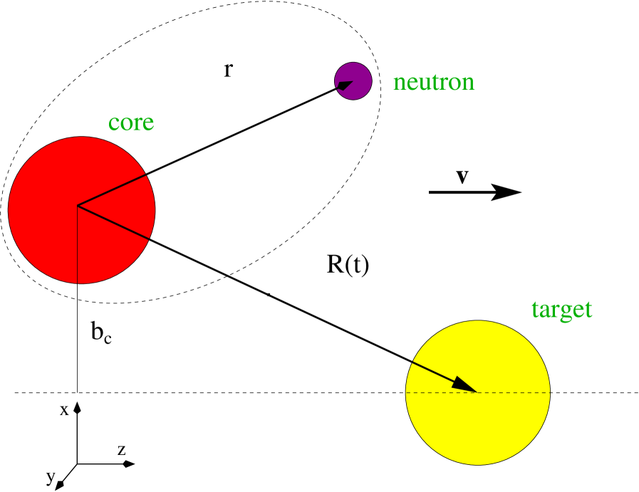
Figure 1: Coordinate system used in the calculations

To first order the inelastic-like excitations can be described by the time dependent perturbation amplitude [4, 34, 35]:

$$A_{fi}={1\over i\hbar}\int_{-\infty}^{\infty}dt\langle\psi_{f}({\bf r},t)|V_{2}({\bf{r-R}}(t))|\psi_{i}({\bf r},t)\rangle,$$ (1)

for a transition from a nucleon bound state $\psi_{i}$ to a final state $\psi_{f}$ which can be a bound state or a continuum state. In this paper we shall treat only continuum final states. $V_{2}$ is the interaction responsible for the neutron transition (cf. Eq. (2.15) of [4]). The potential $V_{2}({\bf{r-R}}(t))$ moves past on a constant velocity path with velocity $v$ in the z-direction with an impact parameter $b_{c}$ in the x-direction in the plane $y=0$. These assumptions and the other discussed in Sec. 2.4 make our semiclassical model valid at beam energies well above the Coulomb barrier. This is in fact the regime in which projectile fragmentation experiments are usually performed (cf. Sec. 4). The coordinate system used in the calculations is shown in Fig.1 and it corresponds to the no-recoil approximation for the core. In the case of the very weakly bound ¹¹Be we will drop this approximation and explicitly take into account core recoil by defining R(t) as the projectile-target relative motion coordinate.

Let $\psi_{i}({\bf r},t)=\phi_{i}({\bf r})e^{-{i\over\hbar}\varepsilon_{i}t}$ be the single particle initial state wave function. Its radial part $\phi_{i}({\bf r})$ is calculated in a potential $V_{WS}(r)$ (cf. Sec. 4) which is fixed in space. In the special case of exotic nuclei the traditional approach to inelastic excitations needs to be modified. For example the final state can be eigenstate of a potential $V_{1}$ modified with respect to $V_{WS}$ because some other particle is emitted during the reaction process as discussed in the introduction. The final state interaction might also have an imaginary part which would take into account the coupling between a continuum state and an excited core. For these reasons our treatment is closer to the formalism used in Ref.[35] to treat rearrangement collisions between heavy ions than to the inelastic excitation formalism of [34]. For initial and final states of different angular momentum our wave functions are trivially orthogonal due to the orthonormality of their angular parts. For transitions conserving the angular momentum of the single particle states we can orthogonalise the initial and final states as suggested by Eq. (8), pag. 303, Ch.V.3, of Ref. [35]. Then

$${\phi_{f}}^{orth}=\phi_{f}-\langle\phi_{i}|\phi_{f}\rangle\phi_{i},$$ (2)

and the first order time dependent perturbation amplitude reads

$$A_{fi}={1\over i\hbar}\int_{-\infty}^{\infty}dtd{\bf r}~{}\phi^{*}_{f}({\bf r})\phi_{i}({\bf r}){e^{i\omega t}}V_{2}({\bf{r-R}}(t))-\Delta A_{fi},$$ (3)

where $\hbar\omega$ is the energy difference between the initial and final states and

$$\Delta A_{fi}={1\over i\hbar}\langle\phi_{f}|\phi_{i}\rangle\int_{-\infty}^{\infty}dtd{\bf r}~{}\phi^{*}_{i}({\bf r})\phi_{i}({\bf r}){e^{i\omega t}}V_{2}({\bf{r-R}}(t)).$$ (4)

Because of the displacement of V₂ with respect to $\phi_{i}$ and in particular for the choice of a $\delta$-potential discussed below, it is expected that the correction due to $\Delta A_{fi}$ will be small. Therefore we shall neglect it in the following.

Now change variables and put $z-vt=z^{\prime}$ or $t=(z-z^{\prime})/v$. The excitation amplitude becomes

$$A_{fi}={1\over i\hbar v}\int_{-\infty}^{\infty}dxdydzdz^{\prime}~{}\phi^{*}_{f}(x,y,z)\phi_{i}(x,y,z){e^{iq(z-z^{\prime})}}V_{2}(x-b_{c},y,z^{\prime}),$$ (5)

where

$$q={{\varepsilon_{f}-\varepsilon_{i}}\over{\hbar v}}.$$ (6)

Then

$$A_{fi}={1\over i\hbar v}\int_{-\infty}^{\infty}dxdydz~{}\phi^{*}_{f}(x,y,z)\phi_{i}(x,y,z){e^{iqz}}\tilde{V}_{2}(x-b_{c},y,q),$$ (7)

where

$$\tilde{V}_{2}(x-b_{c},y,q)=\int_{-\infty}^{\infty}dzV_{2}(x-b_{c},y,z)e^{iqz}.$$ (8)

In our approach the presence of the target represented by this interaction has the effect of perturbing the initial bound state wave function and allow the transition to the continuum by transferring some momentum to the neutron. For this purpose, although the potential $V_{2}(r)$ has a radius of the order of the potential of the target, it is enough to choose a simplified form of the interaction. Therefore we choose $V_{2}(r)$ to be a delta-function potential $V_{2}(r)=v_{2}\delta(x)\delta(y)\delta(z)$, with $v_{2}\equiv$ [MeV fm³]. Then the integrals over x and y can be calculated giving

$$A_{fi}={v_{2}\over i\hbar v}\int_{-\infty}^{\infty}dz~{}\phi^{*}_{f}(b_{c},0,z)\phi_{i}(b_{c},0,z){e^{iqz}}.$$ (9)

The value of the strength $v_{2}$ used in the calculation is discussed in Sec. 5 and in Appendix A. From the above equation it is clear what the effect of the n-target $\delta$-interaction is in a time dependent approach: while in the sudden approach the initial and final state overlap is taken in the whole coordinate space, irrespective of the target and of the beam velocity, here the overlap of the initial and final wave functions is taken at the core-target impact parameter distance on the x-direction which is along the distance of closest approach. The y component is zero (neutron emitted on the reaction plane preferentially) and the z-component, being along the relative velocity axis is boosted by a momentum $q$.

The delta-function potential should be a good approximation if $\gamma{\rm R}_{T}<<1$ and ${\rm kR}_{T}<<1$ where R_T is the radius of the target, $\gamma={\sqrt{-2m\varepsilon_{i}}/\hbar}$ is the decay length of the initial single particle wave function corresponding to the nucleon binding energy $\varepsilon_{i}$ and $k={\sqrt{2m\varepsilon_{f}}/\hbar}$ is the nucleon final momentum in the continuum state. In this case the initial and final wave functions are rather constant over the volume of the target and can be replaced by their values at the center. The second condition is related to the first because the cross section becomes small if $k$ is large compared to $\gamma$ (see Sec. 2.3). We also require that the reaction should be peripheral in the sense that ${\rm R}_{c}+{\rm R}_{T}<{\rm b}_{c}$ where R_c is the projectile core radius. The first condition $\gamma{\rm R}_{T}<<1$ means that the projectile should be a good halo nucleus. Another situation where the delta-function potential is a good approximation is when $\gamma{\rm R}_{T}>>1$. That is the initial state should be strongly bound and the initial state wave function decays rapidly inside the target. Then the $\delta$-potential should be located at the surface of the target. If, for example, V₂(r) is a square well potential with radius R_T and if $\gamma{\rm R}_{T}>>1$, then Eq.(9) can still be used to estimate the breakup with the following changes:

• b_c is replaced by b${}_{c}-{\rm R}_{T}$ i.e. the interaction is located at the surface of the target.

• $v_{2}$ is replaced by $\bar{v}_{2}$ where

  $$\bar{v}_{2}={3\over 2}{v_{2}\over(\gamma-ik)^{2}R_{T}^{2}}.$$ (10)

Thus the strength is reduced and there is an extra phase. The derivation of Eq. (10) is presented in Appendix A.

First we study the simple case where the initial bound state and the final continuum state have $l_{i}=l_{f}=0$, then

$$\phi_{i}(b_{c},0,z)=-{C_{i}\over\sqrt{4\pi}}{e^{-\gamma r}\over r},$$ (11)

$$\phi_{f}(b_{c},0,z)={{C_{f}\over\sqrt{4\pi}}i{k\over 2}}(h^{(-)}_{0}(kr)-Sh^{(+)}_{0}(kr)).$$ (12)

These expressions are the asymptotic forms of the initial and final state wave functions. Their use can be justified when the impact parameter is sufficiently large [3] and $r=\sqrt{b_{c}^{2}+z^{2}}$. $\gamma$ and $k$ are the neutron momenta in the initial and final states already defined. $C_{i}$ is the asymptotic normalization constant of the initial state wave function while $C_{f}=\sqrt{2/L}$ is the normalization constant for the final state. L is a large box radius used to normalize the continuum wave function (cf. Eq. (2.5) of Ref. [29]). The quantity S is the S-matrix representing the final state interaction of the neutron with the projectile core. Then

$$A_{fi}=-{v_{2}\over\hbar v}{C_{i}C_{f}\over 8\pi}\int_{-\infty}^{\infty}dz~{}{e^{-(\gamma-ik)r}-S^{*}e^{-(\gamma+ik)r}\over r^{2}}\cos qz.$$ (13)

Let us define

$$I_{R}=Re\int_{-\infty}^{\infty}dz~{}{e^{-(\gamma-ik)r}\over r^{2}}\cos qz,$$ (14)

and

$$I_{I}=Im\int_{-\infty}^{\infty}dz~{}{e^{-(\gamma-ik)r}\over r^{2}}\cos qz,$$ (15)

such that:

$$I(k,q)=I_{R}+iI_{I}=|I|e^{i\nu}$$ (16)

while

$$\bar{S}=Se^{2i\nu}=e^{2i(\delta+\nu)}$$ (17)

then

$$A_{fi}=C(I-S^{*}I^{*})$$ (18)

and

$$|A_{fi}|^{2}=C^{2}|I|^{2}|1-\bar{S}|^{2}.$$ (19)

Where now $C=-{v_{2}\over\hbar v}{C_{i}C_{f}\over 8\pi}$.

2.1 Wave functions for general $l$

In the general case of a $l_{i}>0$ initial state the amplitude Eq.(1) has to be calculated numerically using, for example, the following forms for the wave functions. For the initial bound state

$$\phi_{i}({\bf r})=-C_{i}i^{l_{i}}\gamma h^{(1)}_{l_{i}}(i\gamma r)Y_{{l_{i}},{m_{i}}}(\theta,\phi).$$ (20)

Due of the strong core absorption discussed in Sec. 2.4 and to get a simple insight at the physics of unbound nuclei, we use in this paper the asymptotic form of the initial state wave function, however the exact wave function, numerical solution of the bound state Schrödinger equation can be used without introducing further complexity in the calculations.

For the final continuum state

$$\phi_{f}({\bf r})=C_{f}k{i\over 2}(h^{(-)}_{l_{f}}(kr)-S_{l_{f}}h^{(+)}_{l_{f}}(kr))Y_{{l_{f}},{m_{f}}}(\theta,\phi).$$ (21)

As it was shown in Ref.[29], in the case of narrow isolated resonances the treatment of the continuum states via the S-matrix is equivalent to the R-matrix formalism.

2.2 Probability spectrum

The probability to excite a final continuum state of energy $\varepsilon_{f}$ is an average over the initial state

$$P_{in}={1\over 2l_{i}+1}\Sigma_{m_{i},m_{f}}|A_{fi}|^{2}$$ (22)

and a sum over the final states. Introducing the quantization condition

$$kL=n\pi,$$ (23)

and the density of final states, according to Ref. [29]

$$\rho(\varepsilon_{f})d\varepsilon_{f}={L\over\pi}{m\over\hbar^{2}k}d\varepsilon_{f},$$ (24)

the probability spectrum reads

$${dP_{in}\over d\varepsilon_{f}}={2\over\pi}{v_{2}^{2}\over\hbar^{2}v^{2}}{C_{i}^{2}}{m\over\hbar^{2}k}{1\over 2l_{i}+1}\Sigma_{m_{i},m_{f}}|1-\bar{S}_{m_{i},m_{f}}|^{2}|I_{m_{i},m_{f}}|^{2},$$ (25)

where now

$$|I_{m_{i},m_{f}}|^{2}=\left|\int_{-\infty}^{\infty}dze^{iqz}i^{l_{i}}\gamma h^{(1)}_{l_{i}}(i\gamma r)Y_{{l_{i}},{m_{i}}}(\theta,0)k{i\over 2}h^{(-)}_{l_{f}}(kr)Y_{{l_{f}},{m_{f}}}(\theta,0)\right|^{2}.$$ (26)

For simplicity the equations in this section are obtained without spin variables in the initial and final states. The generalization including spin is given in Appendix B.

2.3 Approximate evaluation of the integral $I(k,q)$

In order to study the qualitative effects of the final state interaction we proceed now to an approximate evaluation of the integral $I(k,q)$ for $l_{i}=l_{f}=0$. However the calculations presented in Sec. 5 use the exact integrals. For large impact parameters $b_{c}$, write $r=\sqrt{b_{c}^{2}+z^{2}}\approx b_{c}+z^{2}/2b_{c}$. Then

$$I(k,q) \approx {1\over b_{c}^{2}}e^{-(\gamma-ik)b_{c}}\int_{-\infty}^{\infty}dz~{}e^{-(\gamma-ik)z^{2}/2b_{c}}\cos(qz)$$ (27)

$$= {1\over b_{c}^{2}}\sqrt{2\pi b_{c}\over(\gamma-ik)}e^{-(\gamma-ik)b_{c}}\exp\left(-{b_{c}q^{2}\over 2(\gamma-ik)}\right).$$

Hence the phase $\nu$ will be given by

$$\nu = -{1\over 2}arg(\gamma-ik)+kb_{c}-{kb_{c}q^{2}\over 2(\gamma^{2}+k^{2})}$$ (28)

$$= -\footnotesize{1\over 2}arg(\gamma-ik)+kb_{c}\left(1-{\gamma^{2}+k^{2}\over 8{\bar{k}}^{2}}\right)$$

where ${\bar{k}}=mv/\hbar$ and we have used Eq.(6) to obtain $q=(\gamma^{2}+k^{2})/2\bar{k}$. The estimated value of $|I|^{2}$ is

$$|I|^{2} = {1\over b_{c}^{4}}{2\pi b_{c}\over\sqrt{\gamma^{2}+k^{2}}}e^{-2\gamma b_{c}}\exp\left(-\gamma b_{c}{\gamma^{2}+k^{2}\over 4{\bar{k}}^{2}}\right)$$ (29)

$$= {1\over b_{c}^{3}}{2\pi\over\sqrt{\gamma^{2}+k^{2}}}\exp\left(-2\gamma b_{c}\left(1+{q\over 4{\bar{k}}}\right)\right).$$

The above analytical expressions are accurate to within 10$\%$ for impact parameters around the strong absorption radius and for neutron-core energies less that 1.5MeV. The agreement improves for larger impact parameters.

The approximate formulae give rise to simple physical interpretations. The first is that we have an explicit expression for the dependence of $\nu$ on the neutron wave number $k$, the core-neutron impact parameter $b_{c}$ and the adiabaticity parameter $q/{\bar{k}}$. We will discuss some of the effects of the new phase $\nu$ in Sec. 5. $|I|^{2}\sim{e^{-2\gamma b_{c}}\over b_{c}^{3}}$ can be interpreted as an inelastic-like form factor and it is interesting to compare it to the transfer to the continuum form factor ${e^{-2\eta b_{c}}\over b_{c}}$ given in Ref.[29]. The inelastic form factor decreases with the impact parameter much faster than the transfer form factor. This is a well known characteristic for final bound states [35] and it is interesting to see that it persists for final continuum states. Furthermore the slope parameters are in both cases given in lowest order by the initial state decay length $\gamma$.

Finally we make connection with the sudden approximation formula Eq.(20) of Ref.[3] which describes the second step of a two neutron breakup reaction as a resonance decay, when the first neutron has been stripped. In our notation it reads

$${d\sigma\over{d{{\varepsilon_{f}}}}} \sim {1\over k(\gamma^{2}+k^{2})}\left({{k\cos\delta+\gamma\sin\delta}\over\sqrt{\gamma^{2}+k^{2}}}\right)^{2}$$ (30)

$$\sim {1\over k}{|\sin(\delta+\beta)|^{2}\over(\gamma^{2}+k^{2})}$$

where $\beta=arctan(k/\gamma)$. This formalism also predicts the presence of an extra phase shift $\beta$ with respect to the free particle scattering determined by $\delta$ since $|\sin(\delta+\beta)|^{2}={1\over 4}|1-\tilde{S}|^{2}$ and $\tilde{S}=e^{2i(\delta+\beta)}$. Similarly to our case the effect of $\beta$ would be to modify the resonance-like structures. In both cases then $\bar{S}$ and $\tilde{S}$ could be interpreted as off-the-energy-shell S-matrices. On the other hand our additional phase $\nu$ contains an explicit dependence on the impact parameter and we calculate the potential phase shift and S-matrix by an optical model code. Our S-matrix can in principle be complex to allow for core excitation effects. Also it can consistently, and in the same formalism, describe resonant and non-resonant final continuum states of angular momentum $l_{f}=0$ but also $l_{f}>0$. In the latter case, the Breit-Wigner assumption for the line shape of the resonances used in other approaches, is naturally given by the optical model calculation of the factor $|1-\bar{S}|^{2}$ in Eq.(25).

2.4 Cross section

In [35] it was shown that the semiclassical treatment of peripheral quasi-elastic reactions is valid for transfer reactions as well as for (inelastic) projectile excitation and therefore we will apply it in the following by simply substituting $P_{in}(b_{c})$ to $P_{t}(b_{c})$ in the well known formula which gives the cross section in terms of the neutron excitation probability and the core elastic scattering probability. A full description of the treatment of the scattering equation for a nucleus which decays by single neutron breakup following its interaction with another nucleus, can also be found in Refs. [4, 29, 33, 38] where the cross section differential in $\varepsilon_{f}$, the final, continuum, neutron energy is given as

$${d\sigma_{-1n}\over{d{{\varepsilon_{f}}}}}=C^{2}S\int d{\bf b_{c}}{dP_{in}(b_{c})\over d{{\varepsilon_{f}}}}P_{ct}(b_{c}),$$ (31)

(see Eq. (2.3) of [33]) and C²S is the spectroscopic factor for the initial state.

The core survival probability $P_{ct}(b_{c})=|S_{ct}|^{2}$ [33] in Eq.(31) takes into account the peripheral nature of the reaction and naturally excludes the possibility of large overlaps between projectile and target. $P_{ct}$ is defined in terms of a S-matrix function of the core-target distance of closest approach $b_{c}$. A simple parameterisation is $P_{ct}(b_{c})=e^{(-\ln 2exp[(R_{s}-b_{c})/a])}$ [33], where the strong absorption radius R${}_{s}\approx 1.4(A_{p}^{1/3}+A_{t}^{1/3})$ fm is defined as the distance of closest approach for a trajectory that is 50% absorbed from the elastic channel and a=0.6 fm is a diffuseness parameter. The values of R_s thus obtained agree within a few percent with those of the Kox parameterization [36].

Because $P_{in}(b_{c})$ depends on $b_{c}$ trough the form factor $I_{m_{i},m_{f}}$, the final cross sections will get the main contribution from a limited range of impact parameters around the strong absorption radius. As we shall see in the following (cf. figs.7 and 8) this localization makes the tails of the spectra from Eqs.(25) and (31) to decay faster than Eq.(30) towards neutron-core high energies.

3 Two-nucleon breakup

This section introduces the basis for a generalization of Eq.(31) which will be further expanded elsewhere. The goal is to take into account explicitly the presence of a second, stripped, nucleon as in the cases of projectiles like ¹⁴Be which have a two-neutron halo or ¹⁴B in which a proton can also emitted.

We start from hypothesis similar to those leading to Eq.(7) of Ref.[3] which gives, in the case of two-neutron breakup, the one-neutron-core relative momentum distribution when the other neutron is stripped. Let us call (1) the stripped neutron and (2) the neutron detected in coincidence with the core. Following the approximations proposed by Ref.[3] for the coordinate variables, shown in Fig.2, of the core and neutrons with respect to the target one gets: R_1⟂=r_1⟂+b_c and R_2⟂=r_2⟂+b_c, where the heavy-core approximation has been used. r₁ and r₂ are the coordinates of neutron (1) and (2) with respect to the core, while R₁ and R₂ are with respect to the target.

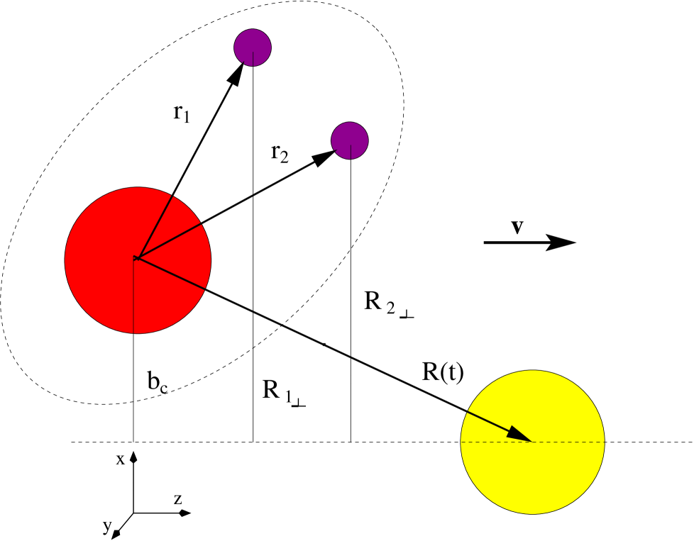
Figure 2: Coordinate system used in the calculations of two-nucleon breakup.

Suppose the initial two-neutron wave function to be given by a product of single particle wave-functions, as in the shell model: $\Psi({\bf r}_{1},{\bf r}_{2})=a_{1}[\phi_{1}({\bf r}_{1})\phi_{2}({\bf r}_{2})]$ with spectroscopic factor $a_{1}^{2}=C^{2}S$. For simplicity we consider here only a $l_{i}=l_{f}=0$ transition and thus we do not include spin wave functions. Then the neutron-core cross section differential in the relative energy is:

$$\frac{d\sigma_{-2n}}{d\varepsilon_{f}}=2C^{2}S\int d^{2}{\bf b}_{c}|S_{ct}(b_{c})|^{2}\frac{dP_{in}(b_{c})}{d\varepsilon_{f}}\int d^{2}{\bf r}_{1\perp}(1-|S_{1}({\bf R}_{1\perp})|^{2})\int dz|\phi_{1}({\bf r}_{1\perp},z)|^{2}.$$ (32)

Where $dP_{in}(b_{c})/{d\varepsilon_{f}}$ is given by Eq.(25) and, similarly to Eq.(31), we are treating the core-target interaction in the eikonal approximation. The $d^{2}{\bf r}_{1\perp}$ integral above gives the neutron (1) stripping probability. For the S₁-matrix we consider a sharp cut-off approximation such that $S_{1}({\bf R}_{1\perp})=0$ if $0<{\rm R}_{1\perp}<{\rm R}_{T}$, while $S_{1}({\rm R}_{1\perp})=1$ if R${}_{1\perp}>{\rm R}_{T}$ and R_T is the target radius.

Thus we obtain a simple expression for the two nucleon breakup cross section, in which one is stripped by the target while the other is elastically scattered and interacts with the core in the final state

$$\frac{d\sigma_{-2n}}{d\varepsilon_{f}}=2C^{2}S\int d^{2}{\bf b_{c}}|S_{ct}(b_{c})|^{2}\frac{dP_{in}(b_{c})}{d\varepsilon_{f}}\int d^{2}{\bf r}_{1\perp}\int dz|\phi_{1}({\bf r}_{1\perp},z)|^{2},$$ (33)

as a product of the neutron (2)-core relative energy distribution and a factor depending on the stripped neutron (1) wave function. For each core-target impact parameter b_c the limits of the integral on r_1⟂ are: b${}_{c}-{\rm R}_{T}<r_{1\perp}<{\rm b}_{c}$.

4 Applications

4.1 The reaction ¹¹Be $\to$ n+¹⁰Be

As a test of our model we calculate the relative energy spectrum n+¹⁰Be obtained by the authors of Ref.[1] in the breakup reaction of ¹¹Be on ¹²C at 70 A.MeV. The structure of ¹¹Be is well known: the valence neutron is bound by 0.503 MeV; the wave function is mainly a 2s state with a spectroscopic factor around 0.8 and there is also a small d_5/2 component. The main d_5/2 strength is in the continuum centered around 1.25 MeV [37]. We have calculated the initial wave function for the s-state in a simple Woods-Saxon potential with strength fitted to the experimental separation energy and whose parameters are: r₀=1.25 fm, a=0.8 fm. As possible final states we have considered only the s, p and d partial waves calculated in the $l$-dependent potentials of Table 1. The delta-function potential strength has been chosen as -4057.59 MeV fm³. The authors of Ref.[1] have shown that the effect of Coulomb breakup is noticeable in their n+¹⁰Be spectrum. We have also included this contribution, calculating it with the method of Margueron et al. [38] which explicitly takes into account the recoil of the core.

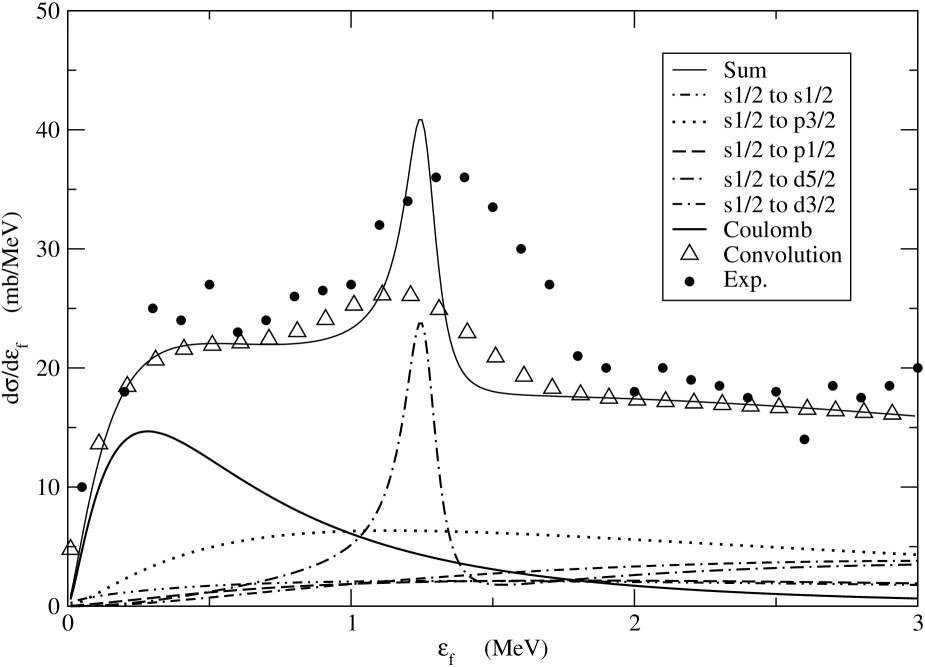
Figure 3: n-¹⁰Be relative energy spectrum, including Coulomb and nuclear breakup for the reaction ¹¹Be+¹²C $\to$ n+¹⁰Be+X at 69 A.MeV. Only the contributions from an s initial state with spectroscopic factor C²S= 0.84 are calculated. The triangles are the total calculated result after convolution with the experimental resolution function. The dots are the experimental points from [1].

Table 1: Woods-Saxon potential parameters for the s, p and d states in the ¹¹Be continuum.

	$l$=0	$l$=1	$l$=2	Vso(MeV)	a (fm)	R (fm)
V0(MeV)	-62.52	-39.74	-63.57	5.25	0.6	2.585

The spectrum of Fig.3 is very similar to the spectrum obtained in Ref.[39] by solving the time-dependent Schrödinger equation numerically, expanding the projectile wave function upon a three-dimensional spherical mesh. Similarly to the present model, a classical, straight line trajectory for the core-target scattering was used in Ref.[39]. Also our n-core potentials are very close to those of Ref.[39] and our $\delta$-interaction strength is consistent with the volume integral of their neutron-target interaction.

We have then folded the calculated spectrum througth the experimental resolution function of Fukuda et al. [1], as given in Ref.[39]

$${d\sigma_{-1n}^{conv}\over{d\varepsilon}}=\int{d\sigma_{-1n}^{theo}\over{d\varepsilon_{f}}}g(\varepsilon_{f}-\varepsilon)d\varepsilon_{f}$$

$$g(\varepsilon_{f}-\varepsilon)={{1}\over{0.48\sqrt{\varepsilon_{f}}}}\exp{\left(-{(\varepsilon-\varepsilon_{f})^{2}\over 0.073\varepsilon_{f}}\right)}$$ (34)

with $\varepsilon_{f}$ the energy in the theoretical calculation. The result is shown in Fig.3 by the triangles. The full curve is the total spectrum, sum of Coulomb and nuclear breakup. Each individual transition, due to the nuclear interaction only, is also shown. The dots are the experimental points from [1]. Our calculations include an initial state spectroscopic factor C²S=0.84. The kind of discrepancy between our calculation and the data in the range 1-2 MeV is very similar to that of the calculations in Ref.[39].

Encouraged by the good agreement of our results with those of Refs.[1] and [39], we conclude that our model is quite reliable to calculate projectile fragmentation including final state interaction with the core and we turn now to the study of more challenging reactions.

4.2 The reactions ¹⁴Be$\to$¹³Be +n and ¹⁴B$\to$¹³Be +p

An interesting unbound nucleus which has recently attracted much attention is ¹³Be. It has been obtained in several different type of experiments with normal and exotic beams but its structure is not clear yet.

One of the aims of this paper is to see whether the neutron-¹²Be relative energy spectra obtained from fragmentation of ¹⁴Be or ¹⁴B would show differences predictable in a theoretical model. Therefore we start by describing briefly the present knowledge of ¹³Be.

4.3 Structure of ¹³Be

The first experimental evidence of ¹³Be was recorded in Ref.[18]. It was the unobserved particle in the two-body reaction ¹⁴C(⁷Li,⁸B) at 82 MeV. A narrow resonance at 2 MeV above the neutron emission threshold was observed in the spectrum of the measured ⁸B ions and it was interpreted as being due to the ground state of ¹³Be. Later on it was identified as a d_5/2 state in the double-charge exchange experiment ¹³C(¹⁴C,¹⁴O) at E_inc=337 MeV [22] and in an inverse kinematics (d,p) transfer reaction at 55 A.MeV [26]: both the missing mass method, from the detected proton spectrum, and the invariant mass spectroscopy, from the measurement of all the decay products from the unbound state were used. The d_5/2 resonance was considered as the ground state of ¹³Be until the experiment of Ref. [23]. This experiment used a stable beam multi-nucleon transfer process ¹⁴C(¹¹B,¹²N)¹³Be in which a lower state, unbound by 800 keV was observed. A spin J=1/2 was suggested but without parity assignment. More recently a broad peak has been obtained in several projectile fragmentation experiments [5, 14, 15, 16] and tentatively identified as a 1/2⁺ state. The experiment of Ref.[14] used fragmentation of ¹⁸O at 80 A.MeV. Neutrons in coincidence with ¹²Be were detected and the broad peak was observed in their relative velocity spectrum. The spectrum was fitted with a virtual s-state of energy 60 keV while in Ref.[5], which used fragmentation of ¹⁴B a virtual s-state could not fit the experimental neutron spectrum. The assumption of an s-resonance of energy 700keV and width 1.3 MeV leads to a good agreement. In Refs.[5, 6, 15, 16] these unbound states of ¹³Be have been populated by breakup of ¹⁴Be or ¹⁴B. Both types of experiments show a low energy peak but only in the breakup of ¹⁴B [5, 6] the other peak at 2 MeV corresponding to the d_5/2 state, is seen clearly. Finally Simon et al. [15] have fitted their spectrum from ¹⁴Be breakup with s, p and d components.

On the other hand the ¹³Be structure is the crucial input of any three-body model describing ¹⁴Be as two neutrons outside an inert ¹²Be core [40, 41, 42]. One then needs to know the n-¹²Be interaction. Assuming in ¹²Be a normal order of shells and an unbound s-ground state of ¹³Be, the d_5/2 resonance, experimentally at 2 MeV, has to be lowered in order to get the experimental two-neutron separation energy in ¹⁴Be [41, 42]. An inversion of 2s-1p_1/2 shells, similar to the inversion in ¹¹Be and ¹⁰Li, was shown to solve this discrepancy [5, 43]. This inversion is due in part to the coupling of the neutron with core collective excited states, inducing in the wave function a component with one neutron coupled to the 2⁺ state of the core. Descouvemont, made a GCM calculation [44, 45]. He expands the ¹³Be and ¹⁴Be wave functions as a superposition of one and two neutrons plus a core of ¹²Be, thus having contributions of components on excited states of the core. He gets an agreement with experimental values of the binding energy of ¹⁴Be and of the d_5/2 resonance energy. His model gives a s-ground state in ¹³Be very weakly bound (100 keV). However due to the uncertainties inherent to any model, this result may not be inconsistent with the experimental evidence for a weakly unbound ¹³Be. These results were confirmed later on by Baye and collaborators in a Lagrange-mesh calculation [46, 47]. Recently Tarutina et al. [48] studied ¹³Be and ¹⁴Be as one and two neutrons outside a deformed core using a hyperspherical harmonics expansion method. They found that both ¹⁴Be and ¹³Be (with an unbound s-ground state) are well described with a large and positive quadrupole deformation. Therefore to disentangle the various theoretical descriptions of ¹³Be and ¹⁴Be one needs more precise experimental information on the structure of both and in particular on their spectroscopic factors.

4.4 Structure of ¹⁴Be and ¹⁴B

These uncertainties in the interpretation of experimental results as compared to structure calculations were at the origin of our motivations to try to understand whether the neutron-¹²Be relative energy spectra obtained from fragmentation of ¹⁴Be or ¹⁴B would show differences predictable in a theoretical model. It is likely that if differences will be found in the experimental results with ¹⁴B and ¹⁴Be beams they could be due to an interplay between structure and reaction effects.

The ground state of ¹⁴Be has spin $J^{\pi}=0^{+}$. In a simple model assuming two neutrons added to a ¹²Be core in its ground state the wave function is:

$$|^{14}Be>=[b_{1}(2s_{1/2})^{2}+b_{2}(1p_{1/2})^{2}+b_{3}(1d_{5/2})^{2}]\otimes|^{12}Be,0^{+}>$$ (35)

Then the bound neutron can be in a 2s, 1p_1/2 or 1d_5/2 state. However, as it has been discussed in the previous section, the situation is much more complicated [40]-[47] and in particular the calculations of Ref. [48] show that there is a large component $(2s_{1/2},1d_{5/2})\otimes|^{12}Be,2^{+}>$ with the core in its low energy 2⁺ state which can modify the neutron distribution.

The ground state of ¹⁴B has spin $J^{\pi}=2^{-}$. In a model where it is described as a neutron-proton pair added to a ¹²Be core in its 0⁺ground state with the proton in the 1p_3/2 shell, its wave function may be written as:

$$|^{14}B>=[a_{1}(p_{3/2},2s_{1/2})+a_{2}(p_{3/2},d_{5/2})]\otimes|^{12}Be,0^{+}>$$ (36)

The present experimental information [49] on ¹⁴B is that the neutron is in a state combination of s and d-components with weights 66% and 30% respectively, while shell model calculations show a similar mixture and no component with an excited state of the core. There are two possibilities for the reaction mechanism. One is that a proton is knocked out in the reaction with the target. The remaining ¹³Be would be left in an unbound s-state with probability $|a_{1}|^{2}$, in a d_5/2-state with probability $|a_{2}|^{2}$. These unbound states would decay showing the s-wave threshold and d-wave resonance effects. As mentioned in the introduction, the second possibility is that the neutron is knocked out first due to its small separation energy and that the proton is stripped from the remaining ¹³B. We show in Sec. 5 that this can also lead to resonance-like effects in the cross section.

4.5 One neutron average potential

The link between reaction theory and structure model is made by the neutron-core potential determining the S-matrix in Eq.(12). Then if the theory fits the position and shape of the continuum n-nucleus energy distribution, obtained for example by a coincidence measurement between the neutron and the core, the parameters of a model potential can be deduced. Our initial bound states are obtained in a simple Woods-Saxon with R= r${}_{0}A^{1/3}$

$$V_{WS}(r)={V_{0}\over{1+e^{(r-R)/a}}}-\left({\hbar\over m_{\pi}c}\right)^{2}{V_{so}\over ar}{e^{(r-R)/a}\over{(1+e^{(r-R)/a})^{2}}}{\mathbf{l\cdot\sigma}}$$ (37)

The depth is adjusted to fit the binding energies given in Table 2 and Fig.10. Other parameters are also given in Table 2.

Table 2: Asymptotic normalization constants C_i(fm^-1/2) for the initial state wave functions of the bound neutron. Potential parameters are: V₀ fitted to give the two energies -0.97 MeV and -1.85 MeV, which are the known neutron binding energies in ¹⁴B and in ¹⁴Be respectively [50]. The other potential parameters are r₀=1.27fm, a=0.75fm, V_so=5.25MeV.

$\varepsilon_{i}$(MeV)	-0.97    -1.85
$l_{i},~{}~{}j_{i}$	Ci(fm-1/2)
0 $~{}~{}{1/2}$	1.31    1.99
1 $~{}~{}{1/2}$	0.55    0.88
2 $~{}~{}{5/2}$	0.17    0.34

To describe the valence neutron in the ¹³Be continuum we assume that the single neutron hamiltonian with respect to ¹²Be has the form

$$h=t+U+iW$$ (38)

where $t$ is the kinetic energy and

$$U(r)=V_{WS}+\delta V$$ (39)

is the real part of the neutron-core interaction. For the time being the imaginary part is taken equal to zero. V_WS is again a Woods-Saxon potential plus spin-orbit whose parameters are given in Table 3, and $\delta$V is a correction [42]:

$$\delta V(r)=16\alpha{e^{{{2(r-R)}/a}}/({1+e^{{{(r-R)}/a}}})^{4}}$$ (40)

which originates from particle-vibration couplings. They are important for low energy states but can be neglected at higher energies. The above form is suggested by a calculation of such couplings using Bohr and Mottelson collective model of the transition amplitudes between zero and one phonon states. Therefore our structure model is not a simple single-particle in a potential model but contains in it the full complexity of single-particle vs. collective couplings. However the fact that such a complexity can be put in a form like Eq.(40) is an added value to our approach. If simple fittings of experimental data will be obtained, then the parameters of a semi-phenomenological potential can be deduced and linked to a more microscopic model. A more realistic treatment would require the description of both bound and unbound states in a three-body model such as in Refs.[51] and [52].

Table 3: Woods-Saxon and spin-orbit potential parameters for the continuum final states.

V0	r0	a	Vso	aso
(MeV)	(fm)	(fm)	(MeV)	(fm)
-39.8	1.27	0.75	6.9	0.75

Table 4 gives the energies and widths of the 1p_1/2 and 1d_5/2 states, chosen according to Ref.[42] with different values of the strength $\alpha$. The widths are obtained from the phase shift variation near resonance energy, according to $d\delta_{j}/d\varepsilon_{f}|_{\varepsilon_{res}}=2/\Gamma_{j}$, once that the resonance energy is fixed [53]. We stress here that while the position of our d_5/2 resonance agrees with the experimental evidences discussed in Sec. 4.3, the position of our 1p_1/2 resonance is only an hypothesis [42, 54].

Table 4: Energies and widths of unbound p- and d-states in ¹³Be and corresponding strength parameters for the $\delta$V potential.

		$\varepsilon_{res}$	$\Gamma_{j}$	$\alpha$
		(MeV)	(MeV)	(MeV)
	1p1/2	0.67	0.28	8.34
	1d5/2	2.0	0.40	-2.36

5 Results

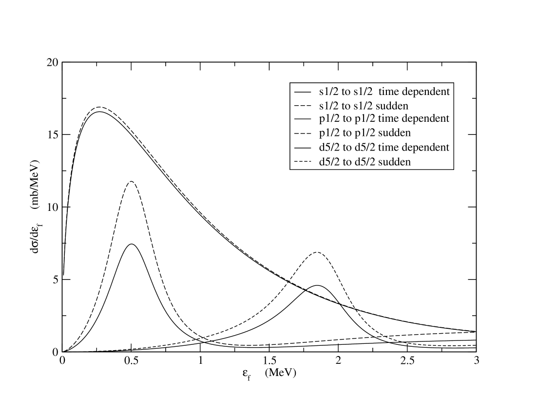
Figure 4: Population of resonances in the n-¹²Be relative energy spectrum. Comparison of sudden (dashed line) and non-sudden (solid line) results for an s $\to$ s transition with peak at 0.25 MeV, p$\to$ p with peak at 0.5 MeV and d$\to$ d transition with peak around 2 MeV. See text for details.

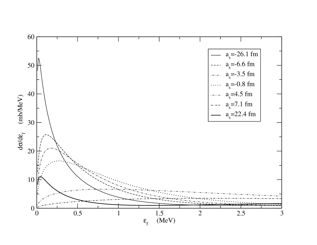
Figure 5: Comparison of results obtained considering a final s-state for the n-¹²Be relative energy spectrum with positive and negative scattering lengths. Scattering lengths are given on the figure and their corresponding $\delta$V potential strengths in Table 5.

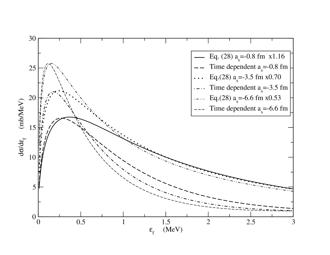
Figure 6: Comparison of time dependent calculation for an s to s transition with results of Eq.(28) using the same optical model phase shifts corresponding to scattering lengths as indicated. For each case we give in the legenda the normalization factor between the two calculations.

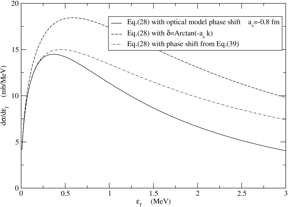
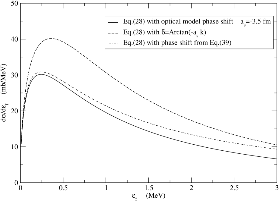
Figure 7: Results of Eq.(28) using three different prescriptions for the phase shifts corresponding to scattering lengths as indicated.

Results obtained with the model outlined in Secs. 2 and 4 will now be discussed. We describe the reaction corresponding to a neutron initially bound in ¹⁴Be or ¹⁴B which is then excited into an unbound state of ¹³Be, assuming that another nucleon has been emitted and stripped by the target, thus not detected in coincidence with the core. The sudden approximation studied in Ref.[3], similar to our q=0 case, was found to be excellent for energy distributions like those discussed in this work.

One of the goals of the present calculations, as far as the reaction model is concerned, is to understand the incident energy dependence of the breakup cross-section and the dependence on the neutron initial binding energy. Related to this is the investigation of the validity of the sudden approximation and the accuracy necessary in calculating the phase shifts. Finally we wish to understand how the presence of p- and d-wave resonances, besides a threshold s-state in the final state, can affect the results.

As a preliminary to a future, more accurate, study of the breakup of ¹⁴Be and ¹⁴B in a fully time dependent method, we consider the knockout of a single neutron from a bound state in a potential, similarly to the previous calculation for ¹¹Be. The calculations in the present section are made with different potentials for the initial and final state. The initial state is bound with a separation energy in the range 1-2 MeV and the final state is unbound. The continuum energies can be adjusted by varying the parameter $\alpha$ in the potential. By changing the strength $\alpha$ of the $\delta$V potential in Eq.(40) we will make also the 2s-state just bound near threshold and see what would be the effect on the continuum spectrum. The delta-interaction strength used in Eq.(8), is $v_{2}$=-8625 MeV fm³. It has been obtained by imposing that this interaction gives the same volume integral as a n-¹²C Woods-Saxon potential of strength -50.5MeV, radius 2.9 fm and diffuseness 0.75 fm. With a diffuseness of 0.5 fm one would obtain $v_{2}$=-6717 MeV fm³. The value $v_{2}$=-7481 MeV fm³ would be obtained from a Woods-Saxon with the same geometry and a depth fitted to give the experimental neutron separation energy in ¹³C.

First we study the differences between results from Eqs.(25) and (31), the sudden approximation limit q=0 of those equations and Eq.(30). In Fig.4 we show the calculation of the differential probability for the transition from a bound s-state to an unbound s-state, a bound p-state to an unbound p-state and a bound d-state to an unbound d-state. The initial state parameters are given in Table 2. The full lines correspond to the case $\varepsilon_{i}$=-1.847 MeV, E_inc=70 A.MeV corresponding to v=11.35 (fm$\times$10²² sec^-1) and q in the range (0.025 $\to$ 0.065) fm^-1. The dashed lines give the q=0 calculations of Eqs.(25) and (31). There is a small difference in the absolute value of the probability and the sudden calculation results have slightly different widths in the s to s case. In the other two cases the differences are noticeable. We have considered only the three transitions keeping $j_{i}=j_{f}$ as it would happen in an extreme sudden transition. Then we studied the effect of the extra phase in Eqs.(25) and (30) on the position of the resonance peaks, and we found that the shift is negligible and would not be noticeable for the range of neutron-core energies discussed here. Also we have calculated for several velocities ranging from 10 to 23 (fm$\times$10²² sec^-1) and found no noticeable differences. On the other hand changing the initial binding energy from -0.97 MeV to -1.85 MeV gives a widening of the distribution and a slight shift of the peak value, as shown in Fig. 10. These two energies are the known neutron binding energies in ¹⁴B and in ¹⁴Be respectively [50]. In this work we have kept the initial separation energy fixed at the value 1.85 MeV, unless otherwise stated. Our conclusion is that for fragmentation reactions such as those discussed here, the sudden approximation q=0 in Eqs.(25) and (31), is well justified from the point of view of the independence from the beam velocity. On the other hand the value of the $\varepsilon_{f}-\varepsilon_{i}$ difference has an important effect on the results when the final energy increases and for states with $l_{f}>0$.

The first peak shown by the experimental spectra of ¹³Be needs to be studied in great detail as it would help determining the ground state angular momentum and parity. In particular, if it is due to an s-state its characteristics will depend on its closeness to threshold. Therefore we study now such a point.

5.1 Low energy s-states

Using the effective range formula [53]

$$k\cot\delta_{0}=-{1\over a_{s}}+{1\over 2}r_{e}k^{2},$$ (41)

in the case of a bound state of small binding energy $\gamma\to 0$ one has

$$-{1\over a_{s}}=-|\gamma|+{1\over 2}r_{e}\gamma^{2}.$$ (42)

Equation (42) has been used [55] also to define an energy of unbound s-states of near zero energy. Such a procedure is reliable when $\gamma R$ is smaller than about 0.5, where $R$ is the radius of the potential. Therefore the effective range formula is accurate only for very low energies. Thus we have fitted the behavior of our s-state phase shifts from the optical model calculation, to Eqs.(41) and (42) and the corresponding parameters are given in Table 5. In the case of a bound state, the effective range values can also consistently be obtained from Eq. (42).

Table 5: Strengths of the s-state $\delta$V potential in Eq.(40) and corresponding scattering lengths, effective range parameter and energy parameter $\epsilon$. The strength of the central Woods-Saxon part is V₀=-39.8 MeV in all cases (cf. Table 3).

	$\alpha$	as	re	$|\epsilon|$
	(MeV)	(fm)	(fm)	(MeV)
	8.0	-0.8	117.0
	4.0	-3.5	17.9
	2.0	-6.6	11.8
	-1.0	-26.1	7.58
	-5.0	22.4	5.9	0.06
	-15.0	7.1	3.8	1.34
	-35.0	4.5	2.7	6.49

Figure 5 shows the influence of the phases $\delta$ and $\nu$ (cf. Eq.(17)) on the breakup cross sections. The results shown correspond to final s-states with positive and negative scattering lengths. Several cases are considered and the corresponding potentials, scattering lengths, and effective ranges are given in Table 5. The scattering length values were obtained from the phase shifts as $a_{s}=-\mathrel{\mathop{lim}\limits_{k\to 0\hskip 1.95999pt}}{tan\delta_{0}\over k}$, and also cross-checked by solving the Schrödinger equation at zero energy. The bound state energies in the last column were obtained from the solution of the Schrödinger equation in each given potential. Notice that the breakup cross sections for potentials with negative scattering lengths are much larger than those with positive scattering lengths. This effect is mainly due to the influence of the phase $\nu$.

The effective phase in Eq.(17) is $\bar{\delta}=\delta+\nu$ and there are interference effects which are especially important for an s-state final state. When $k$ is small $\delta\approx-ka_{s}$ and it depends on the sign of the scattering length, while $\nu\approx k(b_{c}+1/\gamma)$ and it is always positive. The part of the cross section Eq.(31) with the probability Eq.(25) for $l_{f}=0$ and small $k$, depends on the relative sign of a_s and $\nu$ as

$${d\sigma\over{d{{\varepsilon_{f}}}}}\propto|\delta+\nu|^{2}\approx|-ka_{s}+\nu|^{2}.$$ (43)

When a${}_{s}<0$ the cross section is increased relative to the value at $\nu=0$, while for a${}_{s}>0$ it is reduced. This effect is seen clearly in Fig.5. These interference effects can also explain why the cross section for a_s=4.8 fm is larger than for a_s=7.1 fm. Also, the decrease in the positive values of a_s shown in Table 5 corresponds to an increase in the depth of the potential $\delta$V. Fig. 5 shows that the cross section increases for the smallest values of a_s. As the attraction becomes ever stronger the scattering length changes sign and the cross section becomes larger. This effect is due to the influence of a continuum s-state coming close to threshold. When the final potential has a very weakly bound 2s-state with a_s=22.4 fm one sees a very narrow peak close to threshold (thick solid line) while for a_s= 4.5 fm, corresponding to a more strongly bound state, no peak at all, rather a kind of flat bump (double-dotdashed line).

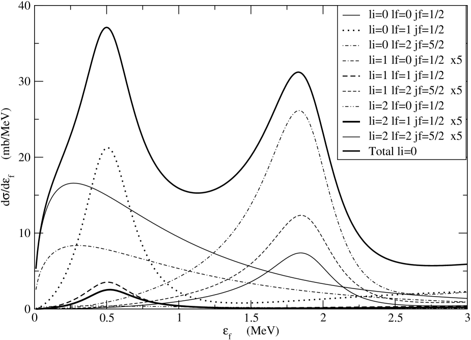
Figure 8: Results obtained including the s, p and d states. Each curve corresponds to just one transition as indicated. The solid curve is the sum of all transitions from the s-bound state. To make them visible some curves have been multiplied by a factor of five as indicated in the legenda.

The calculations presented in Fig. 5 of Ref.[7], did not include the extra phase $\nu$ because the final state interaction with the core of origin was neglected while the final state interaction with respect to the other nucleus was included. In that case the neutron behaved as a free particle in the scattering on the other nucleus. Breakup cross sections depended quite strongly on the magnitude of the scattering length but had a weak dependence on its sign. The reaction mechanism discussed in this paper is instead an inelastic-type of excitation in which the final state interaction is with the core of the projectile and therefore the present formalism shows that the S-matrix in Eq.(19) as well as in Eq.(30) is effectively off-the-energy-shell. In the s $\to$ s case we show also in Fig.6, a comparison between the results just discussed and those obtained using the optical model phase shifts in Eq.(30) and whose absolute values have been normalized to our peaks. As anticipated in Sec. 2.3 and 2.4, the curves from the time dependent model show a faster decrease towards high energies. This is because the form factors in Eq.(25) decrease rapidly and they have large values only for impact parameters close to the strong absorption radius.

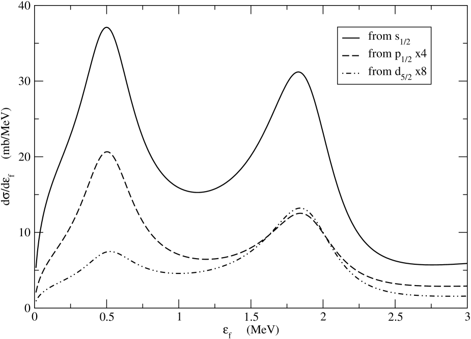
Figure 9: Check of the dependence from the initial state angular momentum. Full curve: sum of transitions from s-initial state. Dashed and dotdashed lines: sum of transitions from p and d-initial states respectively. To make them visible these curves have been multiplied by a factor of four and eight respectively.

Since Eq.(30) is quite simple to implement in an fit to experimental spectra, we have also studied its sensitivity to the choice of the phase shift. Fig.7 shows, for two scattering lengths, results obtained using optical model phase shifts, the second order effective range approximation Eq.(41) with values from Table 5, and the first order phase shift $\delta\simeq-a_{s}k$, as indicated. As expected, the latter approximation is reliable only for extremely small values of the final energy. The second order, effective range parametrization works much better, in particular as the scattering length increases.

5.2 p and d-resonances

Fig. 8 shows results obtained considering three different possibilities for the initial state: the s, p and d orbitals. For each initial state a unit spectroscopic factor is assumed.

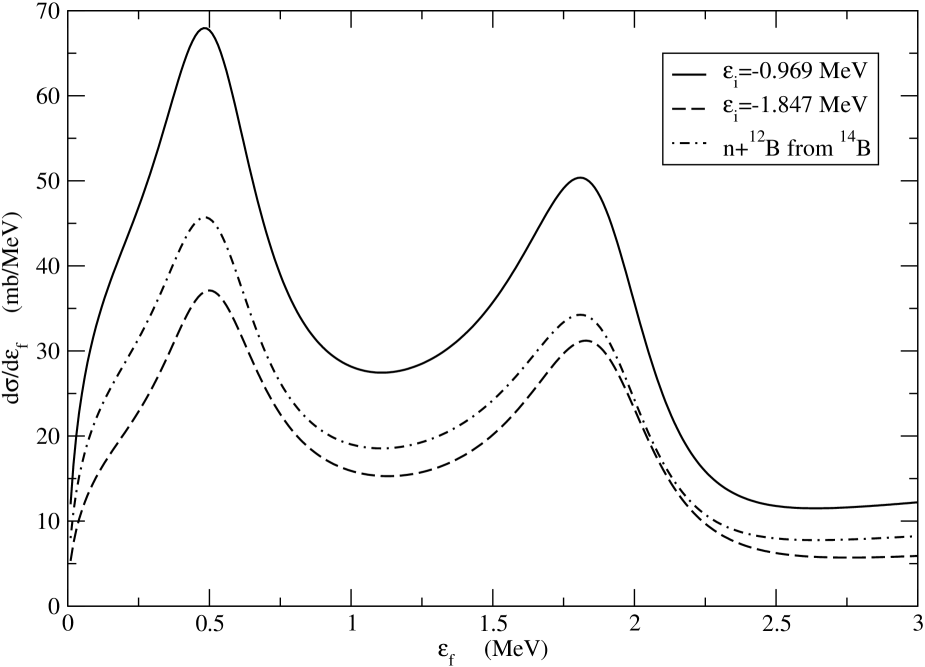
Figure 10: Check of the dependence from the initial binding energy of the sum of transitions from s-initial state. Full curve: $\varepsilon_{i}$= -0.97 MeV as in ¹⁴B; dashed curve: $\varepsilon_{i}$=-1.85 MeV as in ¹⁴Be [50]. Dotdashed line: sum of transitions from s, p and d-initial states including spectroscopic factors of 0.66, 0.04. 0.30 respectively as in ¹⁴B [49] with $\varepsilon_{i}$= -0.97 MeV.

We show the results of the transition bound to unbound from each initial state to each possible unbound state as indicated. Available experimental spectra [23, 26] show that the next group of resonances is located around 4-5 MeV. For this reason higher partial waves have not been included. We have checked that if the d_3/2 and p_3/2 states are calculated in the same potentials as those of the d_5/2 and p_1/2, they would give a noticeable, non resonant, contribution only for a transition from the s initial state. This contribution, not shown in the figures, would constitute a smooth background. The overall effect would be an increase the cross section value of about 10$\%$ around the 0.5 MeV peak and of about 25$\%$ around 2 MeV in Fig.8. The spectrum for Coulomb breakup has also been calculated and found negligible, compared to the other transitions, for the separation energies in ¹⁴Be and ¹⁴B. Therefore it is not included in the figures.

The p and the d-resonance peaks are clearly seen because of the effect of the angular momentum enhancement factor in Eq.(57). As indicated some transition strengths have been multiplied by a factor five to make them visible. It is clear from this figure that the dominant components in the neutron knockout spectrum from ¹⁴Be and ¹⁴B come from the s-wave component in the ground states of those nuclei. Therefore the full curve is the sum of the contributions from the initial s-state alone with unit spectroscopic factor. There can be large peaks due to transitions to the p_1/2 and d_5/2 final state, provided they are centered around the energies we have choosen. The results of Fig. 9 are shown to check the dependence of the transition probability on the initial state angular momentum. The full curve is the sum of transitions from s-initial state. Dashed and dotdashed lines are the sum of transitions from p and d-initial states respectively. Since the transitions from p and d orbitals are negligible, then components in the wave functions of ¹⁴Be or ¹⁴B with a neutron in such angular momentum states will not play much role in the reaction. Thus it is unlikely that any difference in the neutron breakup spectrum due to different mixtures of these configurations in the two parent nuclei will be seen.

To clarify further the latter point, the sum of all transitions from the s-bound state, is shown again in Fig. 10 for two initial binding energies (solid and dashed lines as indicated). Very small changes in the initial binding energy do not give appreciable differences in the final continuum spectra, in particular in the positions of the peaks. They however give differences in the absolute cross section value and in the relative height of the s- and d-state peak. The dotdashed line is the result obtained using the neutron initial binding energy in ¹⁴B, which is -0.969 MeV, and summing transitions from s, p and d-initial states including experimental spectroscopic factors [49] of 0.66, 0.04. 0.30 respectively. According to the simple model for two nucleon breakup presented in Sec. 3, the presence of a 1p_3/2 proton in the initial state would give the same contribution to the breakup of each neutron component and therefore the shape of the spectra should not be modified. On the other hand in the case of ¹⁴Be the two neutrons are in the same state for each component of the initial wave function. Therefore since the p and d wave functions have less pronounced tails, the last integral of Eq.(33), which gives the stripping probability of one of the two neutrons, will naturally diminish the absolute value of the p and d resonances peaks with respect to the final s-state peak.

We notice also that there is a shift between the peaks of the energy spectra and the resonance energies obtained from the phase shifts and given in Table 4. The shift is due to a combined effect of the 1/k factor in Eq.(25), of the matching between initial separation energy, peak energy of the resonance and relative beam energy per nucleon and only in a small measure to the presence of the extra phase $\nu$. The matching effect is manly contained in the slope of the form factor, which to first order is equal to the decay length of the initial state wave function (cf. Eq.(29)). In the ¹¹Be case it is less noticeable because the initial separation energy is very small. The resonance energy was 1.27 MeV while the peak is at 1.25 MeV. For ¹³Be the resonance energies are 0.67 MeV (p-state) and 2 MeV (d-state) while the peaks are at 0.5 MeV and 1.8 MeV respectively. One notices also that the shift increases increasing the resonance energy.

Therefore two differences might be expected in the experimental energy spectra of ¹³Be when produced by ¹⁴Be rather than ¹⁴B projectile fragmentation: a first peak at energy smaller than 0.5 MeV due to the s-continuum state. The s-continuum peak below 0.5MeV, as given by our calculations, can be seen better in Fig.8 and it is due to the s to s transition. If the s initial component would contribute in reality more than the p and d components (we have taken them with equal weights) such a peak could be more evident in the data. Then two more diffuse bumps if the projectile is ¹⁴Be. Two well definite peaks of not too different strength, one centered at 0.5 MeV due to the p_1/2 resonance and another around 2 MeV due to the d_5/2 resonance if the projectile is ¹⁴B. Such an hypothesis agrees also with the conclusion of Ref.[14] of a s-state very close to threshold. The three different experiments [5, 14, 15] would therefore be complementary and allow to determine the characteristics of ¹³Be low energy continuum.

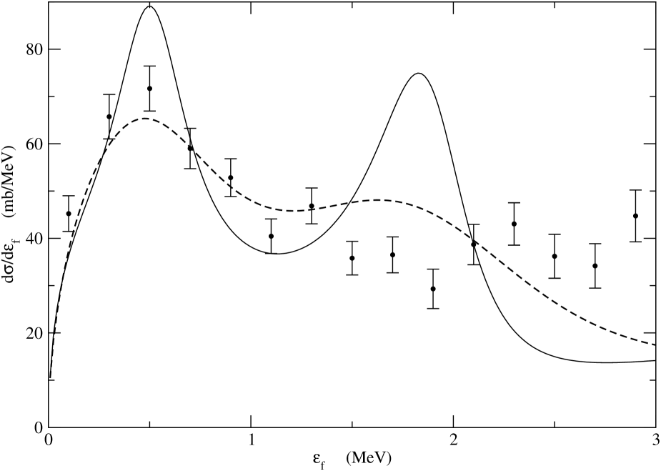
Figure 11: Sum of all transitions from the s initial state with $\varepsilon_{i}$=-1.85 MeV (solid line). Experimental points from H. Simon et al. [56] for the reaction ¹⁴Be+¹²C $\to$ n+¹²Be+X at 250 A.MeV. Dashed line is the folding of the calculated spectrum with the experimental resolution curve.

To give another example of a possible comparison with available data, we show in Fig. 11 the experimental points from H. Simon et al. [56] for the reaction ¹⁴Be+¹²C $\to$ n+¹²Be+X at 250 A.MeV. The normalization factor of the data to mb/MeV is 0.843. The solid line gives the sum of all transitions from the s initial state with $\varepsilon_{f}$=-1.85 MeV (solid line), as in previous figures, renormalized with a factor 2.4. The dashed line is the folding of the calculated spectrum with the experimental resolution curve. Therefore the calculation underestimate the absolute experimental cross section by a factor of 2. In view of the incertitude in the strength of our n-target $\delta$-potential and on the initial state spectroscopic factor which has been taken as unit, we can consider our absolute cross sections quite reasonable.

Finally we wanted to address the issue of possible core excitation effects which in Ref.[48] have been shown to be of fundamental importance for reproducing simultaneously the ¹³Be and ¹⁴Be characteristics. Those effects can be modeled in the present approach by considering a small imaginary part in the neutron-core final optical potential (cf. Eq.(38)). This is a standard procedure for continuum states where most often the potential is also energy dependent [57]. A surface potential of Woods-Saxon derivative form has been taken with strengths W₀ equal to -0.5, -1.0 and -1.5 MeV for the d-state only. The results are shown in Fig. 12. The effect of the imaginary potential is to wash out the d-resonance peak. Several structure models predict indeed the d_5/2 resonance coupled to an excited ¹²Be core. We have found the same smoothing off effect if the s-state is calculated including an imaginary potential. It seems therefore that the spectrum of unbound nuclei could partially reflect the structure of the bound parent nucleus and that reaction mechanism models used to extract structure information should carefully include the effects discussed above. The model presented here seems to be quite promising in this respect.

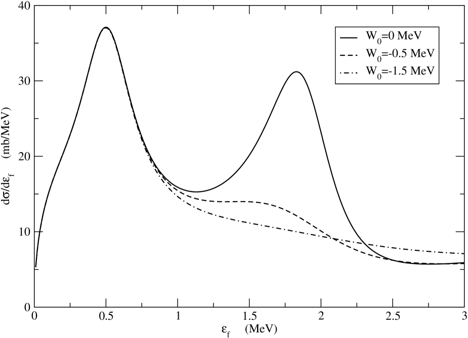
Figure 12: Sum of all transitions from the s initial state with $\varepsilon_{f}$=-1.85 MeV including core excitation via an imaginary part of the optical potential for the d-resonance only.

6 Conclusions and outlook

In this paper we have presented a model to study one neutron excitations from a bound initial state to an unbound resonant state in the neutron-core low energy continuum. This is the process by which unbound nuclei are created and studied via projectile fragmentation experiments [5]-[17, 56].

The model is based on a time dependent perturbation theory amplitude and the final state is described by an optical model S-matrix. It can be considered an evolution with respects to sudden and/or R-matrix theory models. The advantages are that the model can be applied to fragmentation from deeply bound states and to resonant and non resonant, large energy, continuum final states. Also core excitation effects can be modeled by an imaginary part of the neutron-core optical potential.

A related approach has been developed some time ago and applied to the treatment of transfer to the continuum in which, following the interaction between two passing-by nuclei, a neutron from one of them goes from a bound to an unbound state with final state interaction with the other nucleus. Comparison of the present formalism to the transfer to the continuum model shows that in principle projectile fragmentation does not reflect directly the properties of the neutron-core resonances because the reaction mechanism induces an extra phase with respect to the free particle neutron-core phase shift. It means that the measurements would probe an off-the-energy-shell S-Matrix. The distortion effects seem however small and negligible for the cases discussed in this work.

One neutron breakup can be studied in this way but also one step of two neutron breakup of a borromean nucleus. In this paper we have presented some applications to both cases to study the properties of ¹¹Be continuum and of ¹³Be. Our results are in agreement with the conclusions of Ref.[1, 39] for ¹¹Be. Due to the structure inputs we use, in particular the position of the p_1/2 resonance, the ¹³Be continuum spectrum obtained from fragmentation of ¹⁴B or ¹⁴Be shows essentially the effect of the continuum p and d-resonances. The s-state although present in the calculations almost disappears inside the tail of the p-state but it would still determine the ground state spin and parity of ¹³Be. Obviously we cannot be conclusive on the structure of ¹³Be because at the moment we have not attempted to fit experimental data but simply to develop a good reaction model. Furthermore our structure inputs, although reasonable, are extremely simple compared to the complexity of the nucleus under study. However preliminary comparisons seem to indicate the reliability of our model.

We have also shown that the excitation energy spectra of an unbound nucleus might reflect the structure of the parent nucleus from whose fragmentation they are obtained. In particular, in the case of ¹⁴Be fragmentation, the initial state spectroscopic factors are not known experimentally, and the information from structure calculations indicate an important configuration mixing with components coupled to an excited ¹²Be core. Thus the analysis of such spectra is expected to be even more complicated.

However from the point of view of reaction theory, the results obtained here seem promising and we hope to use such a procedure to implement a fit of experimental data on unbound nuclei. At the same time we intend to construct an accurate, second order, fully time dependent theory of two neutron breakup, incorporating properly the time ordering between the two neutrons. In this way we hope to clarify the question of sequential versus simultaneous mechanism implicit in the formation of neutron-core resonance states in reactions like ${}^{11}{\rm Li+X}\to^{10}$Li $\to^{9}$Li+2n [5] or ${}^{14}{\rm Be+X}\to^{13}$Be^∗+n + X$\to^{12}$Be+2n + X, or ${}^{14}{\rm B+X}\to^{13}$ Be^∗+p + X$\to^{12}$Be+n +p + X.

Acknowledgments

We wish to thank Björn Jonson and his collaborators, in particular Leonid Chulkov and Haik Simon, for communicating their results previous to publication, for folding our calculations with their experimental resolution and for an enlightening correspondence. Further discussions with T. Aumann, G. Bertsch, U. Datta-Pramanik, K. Jones, N. Orr, and S. Shimoura, are gratefully acknowledged. This work was inspired by discussions with Takashi Nakamura and the late P. Gregers Hansen at the Spectroscopic Factors workshop, ECT*, Trento, 2004.

Appendix A Modifications to the ${\mathbf{\delta}}$-interaction

Figure 13: Graph of variables used in the calculation of appendix A.

The purpose of this appendix is to justify the use of a $\delta$-interaction as an approximation for the finite range n-target interaction and to derive Eq.(10). We then calculate

$$J=\int_{-\infty}^{\infty}dxdydzdz^{\prime}~{}{e^{-(\gamma-ik)r}\over r^{2}}e^{-iq(z-z^{\prime})}V_{2}(x-b_{c},y,z^{\prime}).$$ (44)

If $\gamma$ is large the integral is concentrated near the surface of V₂(r). To simplify the discussion put $q=0$. Also, as in Sec. 2.3 put

$$e^{-(\gamma-ik)r} \approx e^{-\alpha x}e^{-\alpha(y^{2}+z^{2})/2x}$$ (45)

$$\approx e^{-\alpha x}e^{-\alpha z^{2}/2R_{0}},$$

where $\alpha=\gamma-ik$ and we used the fact that the gaussian term $e^{-\alpha(y^{2}+z^{2})/2x}$ gives the largest contribution at ${\rm R}_{0}={\rm b}_{c}-{\rm R}_{T}$ which is the position of the surface of V₂(r). To simplify further the calculation we have neglected the y-dependence in Eq.(45) but kept the z-dependence so that the integral J will converge. Indicate ${\bar{x}}=x-{\rm R}_{0}=x-({\rm b}_{c}-{\rm R}_{T})$. Take V₂(r) to be a square well potential of depth V₀ and radius R_T. Then

$$\int_{-\infty}^{\infty}~{}V_{2}(x-b_{c},y,z^{\prime})~{}dydz^{\prime}=\pi V_{0}\beta^{2}=2\pi V_{0}R_{T}\bar{x}$$ (46)

where the upper limit of the two dimensional integral is given by $\beta^{2}+(\bar{x}-{\rm R}_{T})^{2}={\rm R}_{T}^{2}$ and $\beta^{2}\approx 2\bar{x}{\rm R}_{T}$.

So that

(47)

The ratio of the integral J to the integral I of Eq.(27) is

$${J\over I}=\left({b_{c}-R_{T}\over b_{c}}\right)^{{1\over 2}}e^{(\gamma-ik)R_{T}}{3\over 2}{v_{2}\over R_{T}^{2}(\gamma-ik)^{2}},$$ (48)

Where we imposed that the strength of the $\delta$-interaction be equal to the volume integral of the square well potential ${v}_{2}={4\over 3}\pi V_{0}R_{T}^{3}$. Thus to represent the effect of a finite range potential by a $\delta$-interaction when $\gamma{\rm R}_{T}>>1$, replace

• (1) ${\rm b}_{c}\to{\rm b}_{c}-{\rm R}_{T}$ i.e. the interaction is at the surface of the target.

• (2) Multiply the strength of the interaction by ${3\over 2}{1\over{\rm R}_{T}^{2}(\gamma-ik)^{2}}$.

This factor is less than one. The change (1) increases the breakup integral, the factor (2) decreases it.

Appendix B Including spin

To include spin variables in the initial and final states is mainly an angular momentum coupling problem. The angle-spin wave function of the initial and final states are

$$\Psi_{i}(j_{i},n_{i},l_{i},\theta,\phi)=\sum_{m_{i}\sigma_{i}}\langle j_{i}n_{i}|l_{i}m_{i}{\frac{1}{2}}\sigma_{i}\rangle Y_{l_{i}m_{i}}(\theta,\phi)\chi_{\sigma_{i}}(\rho)$$ (49)

$$\Psi_{f}(j_{f},n_{f},l_{f},\theta,\phi)=\sum_{m_{f}\sigma_{f}}\langle j_{f}n_{f}|l_{f}m_{f}{\footnotesize{1\over 2}}\sigma_{f}\rangle Y_{l_{f}m_{f}}(\theta,\phi)\chi_{\sigma_{f}}(\rho).$$ (50)

We choose the quantization axis along the y-direction, such that $\phi=0$. Then after integration over $\rho$, the angle spin part of the overlap Eq.(9) is:

$${\cal D}(j_{f}n_{f},j_{i}n_{i}) = \sum_{m_{f}m_{i}\sigma}\langle j_{f}n_{f}|l_{f}m_{f}{\footnotesize{1\over 2}}\sigma\rangle\langle j_{i}n_{i}|l_{i}m_{i}{\footnotesize{1\over 2}}\sigma\rangle Y^{*}_{l_{f}m_{f}}(\theta,0)Y_{l_{i}m_{i}}(\theta,0)$$

$$=\sum_{m_{f}m_{i}\sigma}(-1)^{m_{f}}\langle j_{f}n_{f}|l_{f}-m_{f}{\footnotesize{1\over 2}}\sigma\rangle\langle j_{i}n_{i}|l_{i}m_{i}{\tiny 1\over 2}\sigma\rangle Y_{l_{f}m_{f}}(\theta,0)Y_{l_{i}m_{i}}(\theta,0),$$ (51)

where we have put $Y^{*}_{lm}=(-1)^{m}Y_{l-m}$. Next we use the relation for coupling two spherical harmonics of the same argument and introduce the notation $\hat{i}=\sqrt{2i+1}$

$$Y_{l_{i}m_{i}}(\theta,0)Y_{l_{f}m_{f}}(\theta,0)=\sum_{LM}\langle LM|l_{i}m_{i}l_{f}m_{f}\rangle\langle L0|l_{i}0l_{f}0\rangle{\frac{{\hat{l}_{i}}{\hat{l}_{f}}}{\sqrt{4\pi}{\hat{L}}}}Y_{LM}(\theta,0).$$ (52)

Substituting into the relation for ${\cal D}(j_{f}n_{f},j_{i}n_{i})$ there is a sum of products of three Clebsch-Gordan coefficients which reduces to a product of a Clebsch-Gordan coefficient and a 6-j symbol. Collecting together the terms evaluated above we get:

$${\cal D}(j_{f}n_{f},j_{i}n_{i})=(-)^{f}\sum_{LM}\langle LM|j_{i}n_{i}j_{f}-n_{f}\rangle\langle L0|l_{i}0l_{f}0\rangle\frac{{\hat{l}_{i}}{\hat{l}_{f}}{\hat{j}_{i}}{\hat{j}_{f}}}{\sqrt{4\pi}{\hat{L}}}Y_{LM}(\theta,0)\left\{\begin{array}[]{ccc}l_{i}&l_{f}&L\\ j_{f}&j_{i}&{\footnotesize{1\over 2}}\end{array}\right\}.$$

With the phase $f=n_{f}+l_{f}-j_{f}$

In this scheme the integral Eq.(26)

$$I_{l_{i}m_{i},l_{f}m_{f}}=\int_{-\infty}^{\infty}dze^{iqz}i^{l_{i}}\gamma h^{(1)}_{l_{i}}(i\gamma r)Y_{{l_{i}},{m_{i}}}(\theta,0)k{i\over 2}h^{(-)}_{l_{f}}(kr)Y_{{l_{f}},{m_{f}}}(\theta,0)$$ (55)

is substituted by a new integral $I_{LM}$ defined as

$$I_{LM}=\int_{-\infty}^{\infty}dze^{iqz}i^{l_{i}}\gamma h^{(1)}_{l_{i}}(i\gamma r)k{i\over 2}h^{(-)}_{l_{f}}(kr)Y_{{L,M}}(\theta,0).$$ (56)

Summing over $n_{f}$ and averaging over $n_{i}$ and using the orthogonality of the $\langle LM|j_{i}n_{i}j_{f}n_{f}\rangle$ coefficients while calculating $|{A}(j_{f}n_{f},j_{i}n_{i})|^{2}$ as in Eq.(22) we find that Eq.(25) can be replaced by:

$${dP_{in}\over d\varepsilon_{f}}={2\over\pi}{v_{2}^{2}\over\hbar^{2}v^{2}}{C_{i}^{2}}{m\over\hbar^{2}k}\sum_{LM}C(l_{i},j_{i},l_{f},j_{f};L)|\langle L0|l_{i}0l_{f}0\rangle|^{2}|1-\bar{S}_{LM}|^{2}|I_{LM}|^{2},$$ (57)

where

$$C(l_{i},j_{i},l_{f},j_{f};L)=\frac{(2j_{f}+1)(2l_{i}+1)(2l_{f}+1)}{4\pi(2L+1)}\left\{\begin{array}[]{ccc}l_{i}&l_{f}&L\\ j_{f}&j_{i}&{\footnotesize{1\over 2}}\end{array}\right\}^{2}.$$ (60)

A sum rule for $6-j$ symbols gives

$$\sum_{j_{f}}C(l_{i}j_{i},l_{f},j_{f};L)=\frac{(2l_{f}+1)}{4\pi(2L+1)}.$$ (61)

On the other hand, if in Eq.(25) and (26) or (55) we use the angular momentum coupling formula for spherical harmonics

$$\sum_{m_{i}m_{f}}\langle LM|l_{i}m_{i}l_{f}m_{f}\rangle Y_{l_{i}m_{i}}(\theta,0)Y_{l_{f}m_{f}}(\theta,0)=\langle L0|l_{i}0l_{f}0\rangle\frac{\hat{l_{i}}\hat{l_{f}}}{\sqrt{4\pi}\hat{L}}Y_{LM}(\theta,0),$$ (62)

then the relation between $I_{m_{i}m_{f}}$ and $I_{LM}$ is

$$I_{l_{i}m_{i},l_{f}m_{f}}=\sum_{LM}(-1)^{m_{f}}\langle LM|l_{f}-m_{f}l_{i}m_{i}\rangle\langle L0|l_{i}0l_{f}0\rangle\frac{\hat{l_{i}}\hat{l_{f}}}{\sqrt{4\pi}\hat{L}}I_{LM}$$ (63)

and Eq.(25) is replaced by

$${dP_{in}\over d\varepsilon_{f}}={2\over\pi}{v_{2}^{2}\over\hbar^{2}v^{2}}{C_{i}^{2}}{m\over\hbar^{2}k}\sum_{LM}\frac{(2l_{f}+1)}{4\pi(2L+1)}|\langle L0|l_{i}0l_{f}0\rangle|^{2}|1-\bar{S}_{LM}|^{2}|I_{LM}|^{2},$$ (64)

which could also be obtained using Eq.(61) in (57).

References

- [1] N. Fukuda et al., Phys. Rev. C70, (2004) 054606.
- [2] F. M. Marqués et al., Phys. Rev. C64 (2001) 061301(R). N.Orr, nucl-ex/0201017, Prog. Theor. Phys. Suppl. 146 (2003) 201.
- [3] G. F. Bertsch, K. Hencken and H. Esbensen, Phys. Rev. C57 (1998) 1366.
- [4] A. Bonaccorso and D. M. Brink, Phys. Rev. C43 (1991) 299.
- [5] J. L. Lecouey, Ph. D. thesis, University of Caen, (2002), unpublished and nucl-ex/0310027.
- [6] U. Datta-Pramanik et al., ENAM04 conference, https://www.phy.ornl.gov/enam04/WebTalks/
- [7] G. Blanchon, A. Bonaccorso and N. Vinh Mau, Nucl. Phys. A739 (2004) 259.
- [8] B. Jonson, Phys. Rep. 389 (2004) 1.
- [9] M. Thoennessen, Proceedings the International School of Heavy-Ion Physics, 4th Course: Exotic Nuclei, Erice, May 1997, Eds. R. A. Broglia and P. G. Hansen, (World Scientific, Singapore 1998), pag.269.
- [10] M. Labiche et al. Phys. Rev. Lett. 86 (2001) 600.
- [11] K. Jones, Ph. D. thesis, University of Surrey, (2000), unpublished.
- [12] M. Zinser et al., Nucl. Phys. A619 (1997) 151.
- [13] M. Thoennessen et al., Phys. Rev. C59 (1999) 111.
- [14] M. Thoennessen, S. Yokoyama, and P.G. Hansen, Phys. Rev. C60 (1999) 027303.
- [15] H. Simon et al., Nucl. Phys. A734 (2004) 323.
- [16] T. Nakamura, private communication.
- [17] L. V. Chulkov et al, Phys. Rev. Lett. 79 (1997) 201. L. V. Chulkov and G. Schrieder, Z. Phys. A359 (1997) 231. D. V. Aleksandrov et al., Nucl. Phys. A669 (2000) 51 and references therein.
- [18] D.V. Aleksandrov et al., Sov. J. Nucl. Phys. 37(3) (1983).
- [19] H. G. Bohlen et al. Nucl. Phys. A616 (1997) 254c.
- [20] J. A. Caggiano et al., Phys. Rev. C60 (1999) 064322.
- [21] B. M. Young et al. Phys. Rev. C49 (1994) 279.
- [22] A. N. Ostrowski et al., Z. Phys. A343 (1992) 489.
- [23] A. V. Belozyorov et al., Nucl. Phys. A636 (1998) 419; Phys. Rev. C63 (2000) 014308.
- [24] S. Pita, Thesis University Paris 6 (2000), IPN Orsay IPNO-T-00-11. S. Fortier, Proc. Int. Symposium on Exotic Nuclear Structures ENS 2000, Debrecen (Hungary), Heavy Ion Physics 12 (2001) 255.
- [25] M. Chartier et al., Phys. Lett. B510 (2001) 24.
- [26] A. A. Korsheninnikov et al., Phys. Lett. B343 (1995) 53.
- [27] P. Santi, Ph. D. thesis, University of Notre Dame, (2000), unpublished. P. Santi et al., Phys. Rev. C67 (2003) 024606.
- [28] H. B. Jeppesen for the ISOLDE and REX-ISOLDE collaboration, Nucl. Phys. A 748, (2005) 374.
- [29] A. Bonaccorso and D. M. Brink, Phys. Rev. C38 (1988) 1776.
- [30] A. Bonaccorso and D. M. Brink, Phys. Rev. C44 (1991) 1559.
- [31] A. Bonaccorso, I. Lhenry and T. Suomijärvi, Phys. Rev. C49 (1994) 329.
- [32] A. Bonaccorso, Phys. Rev. C51 (1995) 822.
- [33] A. Bonaccorso, Phys. Rev. C60 (1999) 054604.
- [34] K. Adler, A. Bohr, T.Huus, B. Mottelson and A. Winther, Rev. Mod. Phys. 28 (1956) 432. K. Alder and A. Winther, Electromagnetic Excitation (North-Holland, Amsterdam, 1975).
- [35] R. A. Broglia, and A. Winther, , Addison-Wesley Publ., Redwood City, CA. 1991. Ch.V.
- [36] S. Kox et al., Phys. Rev. C35 (1987) 1678.
- [37] S. Fortier et al., Phys. Lett. B461 (1999) 22 ; T. Aumann et al., Phys. Rev. Lett. 84 (2000) 35 and references therein.
- [38] J. Margueron, A. Bonaccorso and D. M. Brink, Nucl. Phys. A720 (2003) 337.
- [39] P. Capel, D. Baye, Phys. Rev. C70 (2004) 064605.
- [40] G. F. Bertsch and H. Esbensen, Ann. Phys. (N.Y.) 209 (1991) 327.
- [41] I. J. Thompson and M. V. Zhukov, Phys. Rev. C53 (1996) 708.
- [42] N. Vinh Mau and J. C. Pacheco, Nucl. Phys. A607 (1996) 163.
- [43] J. C. Pacheco and N. Vinh Mau, Phys. Rev. C65 044004 (2002).
- [44] P. Descouvemont, Phys. Lett. B331 (1994) 271.
- [45] P. Descouvemont, Phys. Rev. C52 (1995) 704.
- [46] A. Adachour, D. Baye and P. Descouvemont, Phys. Lett. B356 (1995) 445
- [47] D. Baye, Nucl. Phys. A627 (1997) 305.
- [48] T. Tarutina, I. J. Thompson, J. A. Tostevin, Nucl. Phys. A733 (2004) 53.
- [49] V. Guimarães et al., Phys. Rev. C61 (2000) 064609.
- [50] http://nucleardata.nuclear.lu.se/database/masses/
- [51] M. Rodriguez-Gallardo et al, Phys. Rev. C72, (2005) 024007.
- [52] I. J. Thompson et al, Phys. Rev. C47, (1993) R1364.
- [53] C. J. Joachain, Quantum Collision Theory, North-Holland Publishing Company, Amsterdam-Oxford, 1975.
- [54] M. Labiche, F. M. Marques, O. Sorlin, and N. Vinh Mau, Phys. Rev. C60 (1999) 027303.
- [55] J. M. Blatt and V. F. Weisskopf, Theoretical Nuclear Physics, Springer-Verlag, Berlin, 1979.
- [56] H. Simon et al., private communication.
- [57] C. Mahaux and R. Sartor, Adv. Nucl. Phys. 20 (1991) 1.