Beyond the relativistic mean-field approximation (II): configuration mixing of mean-field wave functions projected on angular momentum and particle number

Abstract

The framework of relativistic self-consistent mean-field models is extended to include correlations related to the restoration of broken symmetries and to fluctuations of collective variables. The generator coordinate method is used to perform configuration mixing of angular-momentum and particle-number projected relativistic wave functions. The geometry is restricted to axially symmetric shapes, and the intrinsic wave functions are generated from the solutions of the relativistic mean-field + Lipkin-Nogami BCS equations, with a constraint on the mass quadrupole moment. The model employs a relativistic point-coupling (contact) nucleon-nucleon effective interaction in the particle-hole channel, and a density-independent $\delta$-interaction in the pairing channel. Illustrative calculations are performed for ²⁴Mg, ³²S and ³⁶Ar, and compared with results obtained employing the model developed in the first part of this work, i.e. without particle-number projection, as well as with the corresponding non-relativistic models based on Skyrme and Gogny effective interactions.

I Introduction

In the first part of this work NVR.06 we have extended the theoretical framework of relativistic self-consistent mean-field models to include correlations related to the restoration of broken symmetries and to fluctuations of collective coordinates. In the specific model which has been developed in NVR.06 , the generator coordinate method (GCM) is employed to perform configuration mixing calculations of angular momentum projected wave functions, calculated in a relativistic point-coupling model. The geometry is restricted to axially symmetric shapes, and the mass quadrupole moment is used as the generating coordinate. The intrinsic wave functions are generated from the solutions of the constrained relativistic mean-field + BCS equations in an axially deformed oscillator basis. In order to test the implementation of the GCM and angular momentum projection, a number of illustrative calculations were performed for the nuclei ¹⁹⁴Hg and ³²Mg, in comparison with results obtained in non-relativistic models based on Skyrme and Gogny effective interactions.

In this work we develop the model further by including the restoration of particle number in the wave functions of GCM states, i.e. we restore a symmetry which is broken on the mean-field level by the treatment of pairing correlations either in the BCS approximation, or in the Hartree-Fock-Bogoliubov (HFB) framework. We perform a GCM configuration mixing of angular-momentum and particle-number projected relativistic wave functions. Projection on particle number is crucial whenever the number of correlated pairs becomes small and the density of levels close to the Fermi energy is low, a situation typical for the description of phenomena related to the evolution of shell structure BHR.03 ; VALR.05 : reduction of spherical shell gaps and modifications of magic numbers in nuclei far from stability, occurrence of islands of inversion and coexistence of shapes with different deformations, moments of inertia of superdeformed bands, etc. We thus plan to build a self-consistent relativistic mean-field model in which rotational symmetry and particle-number are restored, and fluctuations of the quadrupole deformation are explicitly taken into account. Such a model can be applied in a quantitative description of shell evolution, and particularly in the treatment of shape coexistence phenomena in nuclei with soft potential energy surfaces.

In Sec. II we outline the relativistic point-coupling model and the Lipkin-Nogami approximate particle number projection, which are used to generate the intrinsic mean-field wave functions with axial symmetry, and introduce the formalism of configuration mixing of angular-momentum and particle-number projected wave functions. In Sec. III the model is tested in a detailed analysis of the spectra of ²⁴Mg, ³²S and ³⁶Ar. In order to illustrate the effects of particle-number projection, we compare the results with those obtained employing the model developed in the first part of this work  NVR.06 , in which the intrinsic wave functions are generated from the solutions of the constrained relativistic mean-field + BCS equations, without particle-number projection. The results are also discussed in comparison with the corresponding nonrelativistic GCM models based on Skyrme and Gogny effective interaction. A brief summary and an outlook for future studies are included in Sec. IV.

II Theoretical framework

II.1 Implementation of the Lipkin-Nogami pairing scheme

In the model that we have developed in Ref. NVR.06 , the intrinsic wave functions are generated from constrained self-consistent solutions of the relativistic mean-field (RMF) equations for the point-coupling (PC) Lagrangian of Ref. BMM.02 . Only basic features of the RMF-PC model are outlined in NVR.06 , and we refer the reader to BMM.02 and references therein, for a complete discussion of the framework of relativistic point-coupling nuclear models. The specific choice of the PC Lagrangian NVR.06 ; BMM.02 defines the mean-field energy of a nuclear system

$${{E}}_{RMF} = \int d{\bm{r}}~{}{\mathcal{E}_{RMF}}(\bm{r})$$ (1)

$$= \sum_{k}{\int d\bm{r}~{}v_{k}^{2}~{}{\bar{\psi}_{k}(\bm{r})\left(-i\bm{\gamma}\bm{\nabla}+m\right)\psi_{k}(\bm{r})}}$$

$$+ \int d{\bm{r}}~{}{\left(\frac{\alpha_{S}}{2}\rho_{S}^{2}+\frac{\beta_{S}}{3}\rho_{S}^{3}+\frac{\gamma_{S}}{4}\rho_{S}^{4}+\frac{\delta_{S}}{2}\rho_{S}\triangle\rho_{S}+\frac{\alpha_{V}}{2}j_{\mu}j^{\mu}+\frac{\gamma_{V}}{4}(j_{\mu}j^{\mu})^{2}+\frac{\delta_{V}}{2}j_{\mu}\triangle j^{\mu}\right.}$$

$$+ \left.\frac{\alpha_{TV}}{2}j^{\mu}_{TV}(j_{TV})_{\mu}+\frac{\delta_{TV}}{2}j^{\mu}_{TV}\triangle(j_{TV})_{\mu}+\frac{\alpha_{TS}}{2}\rho_{TS}^{2}+\frac{\delta_{TS}}{2}\rho_{TS}\triangle\rho_{TS}+\frac{e}{2}\rho_{p}A^{0}\right),$$

where $\psi$ denotes the Dirac spinor field of a nucleon, and the the local isoscalar and isovector densities and currents

$$\rho_{S}({\bm{r}}) = \sum_{k}v_{k}^{2}~{}\bar{\psi}_{k}({\bm{r}})\psi_{k}({\bm{r}})~{},$$ (2)

$$\rho_{TS}({\bm{r}}) = \sum_{k}v_{k}^{2}~{}\bar{\psi}_{k}({\bm{r}})\tau_{3}\psi_{k}({\bm{r}})~{},$$ (3)

$$j^{\mu}({\bm{r}}) = \sum_{k}v_{k}^{2}~{}\bar{\psi}_{k}({\bm{r}})\gamma^{\mu}\psi_{k}({\bm{r}})~{},$$ (4)

$$j^{\mu}_{TV}({\bm{r}}) = \sum_{k}v_{k}^{2}~{}\bar{\psi}_{k}({\bm{r}})\gamma^{\mu}\tau_{3}\psi_{k}({\bm{r}})~{},$$ (5)

are calculated in the no-sea approximation: the summation runs over all occupied states in the Fermi sea, i.e. only occupied single-nucleon states with positive energy explicitly contribute to the nucleon self-energies. $v_{k}^{2}$ denotes the occupation factors of single-nucleon states. In Eq. (1) $\rho_{p}$ is the proton density, and $A^{0}$ denotes the Coulomb potential.

In addition to the self-consistent mean-field potential, for open-shell nuclei pairing correlations have to be included in the energy functional. In this work we do not consider nuclear systems very far from the valley of $\beta$-stability, and therefore a good approximation for the treatment of pairing correlations is provided by the BCS formalism. Following the prescription from Ref. BMM.02 , we use a $\delta$-interaction in the pairing channel, supplemented with a smooth cut-off determined by the Fermi function of single-particle energies $\epsilon_{k}$ KBF.90 :

$$f_{k}^{2}=\frac{1}{1+e^{(\epsilon_{k}-\lambda_{\tau}-\Delta E_{\tau})/\mu_{\tau}}}\;,$$ (6)

where $\lambda_{\tau}$ is the Fermi energy for neutrons ($\tau=n$) or protons ($\tau=p$). $f^{2}_{k}$ is used in the evaluation of the pairing density

$$\kappa_{\tau}(\bm{r})=-2\sum_{k>0}f_{k}u_{k}v_{k}\psi_{k}(\bm{r})^{\dagger}\psi_{k}(\bm{r})\;,$$ (7)

where the summation runs for $\tau=n(p)$ over neutron (proton) single-particle states. The cut-off parameters $\Delta E_{q}$ and $\mu_{q}=\Delta E_{q}/10$ are adjusted to the density of single-particle levels in the vicinity of the Fermi energy. In particular, the sum of the cut-off weights approximately includes one additional shell of single-particle states above the Fermi level

$$\sum_{k>0}2f_{k}=N_{\tau}+1.65N_{\tau}^{2/3}\;,$$ (8)

where $N_{\tau}$ denotes number of neutrons (protons) in a specific nucleus. The pairing contribution to the total energy is given by

$${E}_{pair}^{\tau}=\int{\mathcal{E}_{pair}^{\tau}(\bm{r})d\bm{r}}=\frac{V_{\tau}}{4}\int{\kappa_{\tau}^{*}(\bm{r})\kappa_{\tau}(\bm{r})d\bm{r}}\;,$$ (9)

where $V_{n(p)}$ denotes the strength parameter of the pairing interaction for neutrons (protons). Finally, the expression for the total energy reads

$$E_{tot}=\int{\left[\mathcal{E}_{RMF}(\bm{r})+\mathcal{E}_{pair}^{p}(\bm{r})+\mathcal{E}_{pair}^{n}(\bm{r})\right]d\bm{r}}\;,$$ (10)

and the center-of-mass correction is included by adding the expectation value

$$E_{cm}=-\frac{\langle\hat{\bm{P}}_{cm}^{2}\rangle}{2mA}\;,$$ (11)

to the total energy, where $\bm{P}_{cm}$ denotes the total momentum of the nucleus.

The principal disadvantage of describing pairing correlations in the BCS approximation is that the resulting wave function is not an eigenstate of the particle number operator. More precisely, the BCS ground state contains admixtures of particle-number eigenstates with a relative spread of order $1/\sqrt{N}$, where $N$ denotes the average number of valence particles. The ideal solution, of course, is to perform particle number projection from the BCS state before variation. This procedure is technically rather complicated and very much time consuming, and therefore it is usual to employ the Lipkin-Nogami (LN) approximation to the exact particle number projection Lip.60 ; Nog.64 ; FO.97 . In this work the LN method is implemented in terms of local density functionals of the effective interaction, as developed in Refs. RNB.96 ; VER.96 ; VER.97 ; BRR.00 .

The Lipkin-Nogami equations are obtained from the variation of the functional

$$\mathcal{K}=\mathcal{E}_{tot}-\sum_{\tau=n,p}{\lambda_{1,\tau}\langle\hat{N}_{\tau}\rangle+\lambda_{2,\tau}\langle\hat{N}_{\tau}^{2}\rangle}\;,$$ (12)

with respect to the single-particle states $\bar{\psi}_{k}$ and the occupation amplitudes $v_{k}$. $\mathcal{E}_{tot}$ is the total energy functional of Eq. (10). The resulting expression for the occupation probabilities can be cast into the standard BCS formula

$$v_{k}^{2}=\frac{1}{2}\left[1-\frac{\epsilon^{\prime}_{k}-\lambda_{\tau}}{\sqrt{(\epsilon^{\prime}_{k}-\lambda_{\tau})^{2}+f_{k}^{2}\Delta_{k}^{2}}}\right]\;,$$ (13)

where $\epsilon^{\prime}_{k}=\epsilon_{k}+4\lambda_{2,\tau}v_{k}^{2}$ denotes the renormalized single-particle energy, and $\lambda_{\tau}=\lambda_{1,\tau}+4\lambda_{2,\tau}(N_{\tau}+1)$ is the generalized Fermi energy. $\lambda_{1,\tau}$ is determined by a particle number subsidiary condition such that the expectation value of the particle number operator equals the given number of nucleons. The state-dependent single-particle gaps are defined as the matrix elements

$$\Delta_{k}=\int{d\bm{r}\psi_{k}^{\dagger}(\bm{r})\Delta_{\tau}(\bm{r})\psi_{k}(\bm{r})}\;,$$ (14)

of the local pair potential

$$\Delta_{\tau}(\bm{r})=\frac{1}{2}V_{\tau}\kappa_{\tau}(\bm{r})\quad\quad(\tau\equiv n,p)\;.$$ (15)

While the quantities $\lambda_{1,\tau}$ represent the Lagrange multipliers used to constrain the average particle numbers, the value of the parameters $\lambda_{2,\tau}$ are determined from

$$\lambda_{2,\tau}=\frac{\langle\hat{H}\Delta\hat{N}_{2,\tau}^{2}\rangle}{\langle\hat{N}_{\tau}^{2}\Delta\hat{N}_{2,\tau}^{2}\rangle}\;,$$ (16)

where $\hat{N}_{2,\tau}$ is the term of the particle number operator which projects onto two-quasiparticle states

$$\hat{N}_{2,\tau}=2\sum_{k>0}{u_{k}v_{k}(\alpha_{k}^{\dagger}\alpha_{\bar{k}}^{\dagger}+\alpha_{\bar{k}}\alpha_{k})}\;,$$ (17)

and $\Delta\hat{N}_{2,\tau}^{2}=\hat{N}_{2,\tau}^{2}-\langle\hat{N}_{2,\tau}^{2}\rangle$ denotes its variance. The evaluation of the parameters $\lambda_{2,\tau}$ is described in the Appendix.

After approximate particle-number projection the total binding energy reads

$${E}_{LN}={E}_{tot}-\sum_{\tau=n,p}\lambda_{2,\tau}\langle(\Delta\hat{N}_{2,\tau})^{2}\rangle\;.$$ (18)

The strength of the pairing interaction can be determined by comparing the average pairing gaps with empirical gaps obtained from nuclear masses. The average gap is given by the summation over occupied states with either the occupation probability $v_{k}^{2}$ as the weighting factor DFT.84

$$\langle v^{2}\Delta\rangle_{\tau}=\frac{\sum_{k>0}f_{k}v_{k}^{2}\Delta_{k}}{\sum_{k>0}f_{k}v_{k}^{2}}\;,$$ (19)

or the factor $u_{k}v_{k}$ BRR.00

$$\langle uv\Delta\rangle_{\tau}=\frac{\sum_{k>0}f_{k}u_{k}v_{k}\Delta_{k}}{\sum_{k>0}f_{k}u_{k}v_{k}}\;.$$ (20)

The corresponding expressions for the (approximately) particle-number projected average pairing gaps read CDH.96 ; BRR.00 :

$$\langle v^{2}\Delta\rangle_{\tau}^{LN}=\langle v^{2}\Delta\rangle_{\tau}+\lambda_{2,\tau}\;,$$ (21)

$$\langle uv\Delta\rangle_{\tau}^{LN}=\langle uv\Delta\rangle_{\tau}+\lambda_{2,\tau}\;.$$ (22)

The local densities and currents which define the energy functional refer to the intrinsic state, and are therefore computed from the Eqs. (2) – (5). On the other hand, the densities used to evaluate physical observables, such as the mass quadrupole moment, must correspond to the (approximately) particle-number projected state. The LN density is simply computed by replacing the occupation probabilities $v_{k}^{2}$, with the LN occupation coefficients BHB.89 ; QRM.90

$$w_{k}=v_{k}^{2}+\frac{u_{k}^{2}v_{k}^{2}\overline{u^{2}v^{2}}\left[(v_{k}^{2}-u_{k}^{2})\overline{u^{2}v^{2}}-\overline{u^{2}v^{2}(v^{2}-u^{2})}\right]}{\overline{u^{2}v^{2}}\;\overline{u^{2}v^{2}(v^{2}-u^{2})^{2}}-[\overline{u^{2}v^{2}(v^{2}-u^{2})}]^{2}+2\overline{u^{2}v^{2}}[(\overline{u^{2}v^{2}})^{2}-\overline{u^{4}v^{4}}]}\;,$$ (23)

where $\overline{x}$ denotes half of the trace

$$\overline{x}=\sum_{k>0}x_{k}\;.$$ (24)

We note that LN-corrected quadrupole moments will be used in the constrained self-consistent relativistic mean-field calculations (see Eq. 26).

In this work we only consider even-even nuclei that can be described by axially symmetric shapes. In addition to axial symmetry and parity, symmetry with respect to the operator $e^{-i\pi\hat{J}_{y}}$, and time-reversal invariance are imposed as self-consistent symmetries. The single-nucleon Dirac eigenvalue equation is solved by expanding the large and small components of the nucleon spinor $\psi_{i}$ in terms of eigenfunctions of an axially symmetric harmonic oscillator potential (see Ref. GRT.90 for details).

II.2 Configuration mixing of mean-field solutions projected on angular momentum and particle number

Correlation effects related to the restoration of broken symmetries and to fluctuations of collective coordinates can be taken into account by performing configuration mixing calculations of projected states. The generator coordinate method (GCM), which uses a set of mean-field states $\left|\phi(q)\right\rangle$ that depend on a collective coordinate $q$, provides a very efficient procedure for the construction of the trial wave function RS.80 :

$$\left|\Psi_{\alpha}\right\rangle=\sum_{j}{f_{\alpha}(q_{j})\left|\phi(q_{j})\right\rangle}\;.$$ (25)

In this work the basis states $\left|\phi(q)\right\rangle$ are Slater determinants of single-nucleon states generated by solving the constrained relativistic mean-field + LNBCS equations, with the quadrupole moment as the generating coordinate $q$. For an axially deformed nucleus the map of the energy surface as a function of deformation is obtained by imposing a constraint on the mass quadrupole moment. The method of quadratic constraint uses an unrestricted variation of the function

$$\langle\mathcal{K}\rangle~{}+~{}\frac{C}{2}\left(\langle\hat{Q}\rangle-~{}q\right)^{2}\;,$$ (26)

where $\langle\mathcal{K}\rangle$ is the energy functional of Eq. (12), $\langle\hat{Q}\rangle$ denotes the expectation value of the mass quadrupole operator, $q$ is the deformation parameter, and $C$ is the stiffness constant.

The axially deformed mean-field breaks rotational symmetry, and the particle number is only approximately restored with the Lipkin-Nogami procedure, i.e. the basis states $\left|\phi(q)\right\rangle$ are not eigenstates of the total angular momentum and particle number operators. Therefore, in order to be able to compare model predictions with data, we must construct states with good angular momentum and particle number, by performing projections from the mean-field plus LNBCS solutions

$$\left|\Psi_{\alpha}^{JM}\right\rangle=\sum_{j,K}{f_{\alpha}^{JK}(q_{j})\hat{P}_{MK}^{J}\hat{P}^{Z}\hat{P}^{N}\left|\phi(q_{j})\right\rangle}~{}.$$ (27)

The particle-number projection operators read

$$\hat{P}^{N}=\frac{1}{2\pi}\int_{0}^{2\pi}{d\varphi_{n}e^{i(\hat{N}-N)\varphi_{n}}}~{},\quad\hat{P}^{Z}=\frac{1}{2\pi}\int_{0}^{2\pi}{d\varphi_{p}e^{i(\hat{Z}-Z)\varphi_{p}}}~{}.$$ (28)

where $\hat{N}(\hat{Z})$ is the number operator for neutrons (protons), and $N(Z)$ denotes the number of neutrons (protons).

The angular momentum projection operator is defined by

$$\hat{P}^{J}_{MK}=\frac{2J+1}{8\pi^{2}}\int{d\Omega D_{MK}^{J*}(\Omega)\hat{R}(\Omega)}\;,$$ (29)

where the integration is performed over the three Euler angles $\alpha$, $\beta$, and $\gamma$. $D_{MK}^{J}(\Omega)=e^{-iM\alpha}d^{J}_{MK}(\beta)e^{-iK\gamma}$ is the Wigner function VMK.88 , and $\hat{R}(\Omega)=e^{-i\alpha\hat{J}_{z}}e^{-i\beta\hat{J}_{y}}e^{-i\gamma\hat{J}_{z}}$ is the rotation operator.

The weight functions $f_{\alpha}^{JK}(q_{j})$ are determined by requiring that the expectation value of the energy is stationary with respect to an arbitrary variation $\delta f_{\alpha}^{JK}$:

$$\delta E^{J}=\delta\frac{\left\langle\Psi_{\alpha}^{JM}\right|\hat{H}\left|\Psi_{\alpha}^{JM}\right\rangle}{\left\langle\Psi_{\alpha}^{JM}\right|\Psi_{\alpha}^{JM}\rangle}=0\;.$$ (30)

This leads to the Hill-Wheeler equation HW.53 :

$$\sum_{j,K}f_{\alpha}^{JK}(q_{j})\left(\left\langle\phi(q_{i})\right|\hat{H}\hat{P}_{MK}^{J}\hat{P}^{N}\hat{P}^{Z}\left|\phi(q_{j})\right\rangle-E^{J}_{\alpha}\left\langle\phi(q_{i})\right|\hat{P}_{MK}^{J}\hat{P}^{N}\hat{P}^{Z}\left|\phi(q_{j})\right\rangle\right)=0\;.$$ (31)

The restriction to axially symmetric configurations ($\hat{J}_{z}\left|\phi(q)\right\rangle=0$) simplifies the problem considerably, because in this case the integrals over the Euler angles $\alpha$ and $\gamma$ can be performed analytically. In addition, the symmetry with respect to the operator $e^{-i\pi\hat{J}_{y}}$ reduces the integration interval over the Euler angle $\beta$ from $[0,\pi]$ to $[0,\pi/2]$. For an arbitrary multipole operator $\hat{Q}_{\lambda\mu}$ one thus finds

$$\left\langle\phi(q_{i})\right|\hat{Q}_{\lambda\mu}\hat{P}_{MK}^{J}\hat{P}^{N}\hat{P}^{Z}\left|\phi(q_{j})\right\rangle=(2J+1)\frac{1+(-1)^{J}}{2}\delta_{M-\mu}\delta_{K0}\times\frac{1}{(2\pi)^{2}}$$

$$\int_{0}^{2\pi}d\varphi_{n}\int_{0}^{2\pi}d\varphi_{p}\int_{0}^{\pi/2}\sin\beta d_{-\mu 0}^{J*}(\beta)\left\langle\phi(q_{i})\right|\hat{Q}_{\lambda\mu}e^{-i\beta\hat{J}_{y}}e^{i(\hat{N}-N)\varphi_{n}}e^{i(\hat{Z}-Z)\varphi_{p}}\left|\phi(q_{j})\right\rangle d\beta\;.$$ (32)

We note that this expression is defined only for even values of the angular momentum $J$. The norm overlap kernel

$$\mathcal{N}^{J}(q_{i},q_{j}) = \left\langle\phi(q_{i})\right|\hat{P}_{MK}^{J}\hat{P}^{N}\hat{P}^{Z}\left|\phi(q_{j})\right\rangle=$$ (33)

$$(2J+1)\frac{1+(-1)^{J}}{2}\delta_{M0}\delta_{K0}\frac{1}{(2\pi)^{2}}\int_{0}^{2\pi}d\varphi_{n}\int_{0}^{2\pi}d\varphi_{p}\times$$

$$\int_{0}^{\pi/2}{\sin{\beta}d_{00}^{J*}(\beta)\left\langle\phi(q_{i})\right|e^{-i\beta\hat{J}_{y}}e^{i(\hat{N}-N)\varphi_{n}}e^{i(\hat{Z}-Z)\varphi_{p}}\left|\phi(q_{j})\right\rangle d\beta}\;,$$

can be evaluated by using the fact, that $\left|\phi(q_{j})\right\rangle$ is a product of a neutron- and a proton Slater determinant and the generalized Wick theorem OY.66 ; BB.69 ; BDF.90 ; VHB.00 :

$$n(q_{i},q_{j};\beta,\varphi_{\tau}) \equiv \left\langle\phi(q_{i})\right|e^{-i\beta\hat{J}_{y}}e^{i\hat{N}_{\tau}\varphi_{\tau}}\left|\phi(q_{j})\right\rangle=\pm\sqrt{det~{}\mathcal{N}_{ab}(q_{i},q_{j};\beta,\varphi_{\tau})}\;,$$ (34)

for $\tau=n,p$. The overlap matrix is defined as

$$\mathcal{N}_{ab}(q_{i},q_{j};\beta,\varphi_{\tau})=u_{a}(q_{i})R_{ab}(q_{i},q_{j};\beta)u_{b}(q_{j})+v_{a}(q_{i})R_{ab}(q_{i},q_{j};\beta)v_{b}(q_{j})e^{2i\varphi_{\tau}}\;,$$ (35)

where $u$ and $v$ denote the BCS occupation probabilities, and the elements of the matrix $R$ read

$$R_{ab}(q_{i},q_{j};\beta)=\int{\psi_{a}^{\dagger}(\bm{r};q_{i})e^{-i\beta\hat{J}_{y}}\psi_{b}(\bm{r};q_{j})d\bm{r}}\;.$$ (36)

We note that the global phase of the overlap in Eq. (34) is determined by using the procedure described in Ref. VHB.00 . The details of the evaluation of the matrix $R$ can be found in Ref. NVR.06 .

The Hamiltonian kernel

$$\mathcal{H}^{J}(q_{i},q_{j}) = \left\langle\phi(q_{i})\right|\hat{H}\hat{P}_{MK}^{J}\hat{P}^{N}\hat{P}^{Z}\left|\phi(q_{j})\right\rangle=$$ (37)

$$(2J+1)\frac{1+(-1)^{J}}{2}\delta_{M0}\delta_{K0}\frac{1}{(2\pi)^{2}}\int_{0}^{2\pi}d\varphi_{n}\int_{0}^{2\pi}d\varphi_{p}\times$$

$$\int_{0}^{\pi/2}\sin{\beta}d_{00}^{J*}(\beta)\left\langle\phi(q_{i})\right|\hat{H}e^{-i\beta\hat{J}_{y}}e^{i(\hat{N}-N)\varphi_{n}}e^{i(\hat{Z}-Z)\varphi_{p}}\left|\phi(q_{j})\right\rangle d\beta\;,$$

can be calculated from the mean-field energy functional Eq. (1), provided the modified densities OY.66 ; BB.69 ; BDF.90 ; VHB.00

$$\tau^{\tau}(\bm{r};q_{i},q_{j},\beta,\varphi_{\tau}) = \sum_{a,b}v_{a}(q_{i})v_{b}(q_{j})e^{2i\varphi_{\tau}}\mathcal{N}_{ba}^{-1}(q_{i},q_{j};\beta)\times$$ (38)

$$\bar{\psi}_{a}(\bm{r};q_{i})(-i\bm{\gamma}\bm{\nabla}+m)e^{-i\beta\hat{J}_{y}}\psi_{b}(\bm{r};q_{j})\;,$$

$$\rho_{S}^{\tau}(\bm{r};q_{i},q_{j},\beta,\varphi_{\tau}) = \sum_{a,b}v_{a}(q_{i})v_{b}(q_{j})e^{2i\varphi_{\tau}}\mathcal{N}_{ba}^{-1}(q_{i},q_{j};\beta)\bar{\psi}_{a}(\bm{r};q_{i})e^{-i\beta\hat{J}_{y}}\psi_{b}(\bm{r};q_{j})\;,$$ (39)

$$j_{\mu}^{\tau}(\bm{r};q_{i},q_{j},\beta,\varphi_{\tau}) = \sum_{a,b}v_{a}(q_{i})v_{b}(q_{j})e^{2i\varphi_{\tau}}\mathcal{N}_{ba}^{-1}(q_{i},q_{j};\beta)\bar{\psi}_{a}(\bm{r};q_{i})\gamma_{\mu}e^{-i\beta\hat{J}_{y}}\psi_{b}(\bm{r};q_{j})\;,$$ (40)

are used when evaluating the expression

$$h(q_{i},q_{j};\beta,\varphi_{n},\varphi_{p}) \equiv \left\langle\phi(q_{i})\right|\hat{H}e^{-i\beta\hat{J}_{y}}e^{i\hat{N}\varphi_{n}}e^{i\hat{Z}\varphi_{p}}\left|\phi(q_{j})\right\rangle=\int{\mathcal{E}_{tot}(\bm{r};q_{i},q_{j},\beta,\varphi_{n},\varphi_{p})d\bm{r}}.$$ (41)

The computational task of evaluating the Hamiltonian and norm overlap kernels can be reduced significantly if one realizes that states with very small occupation probabilities give negligible contributions to the kernels, and hence such states can be excluded from the calculation BDF.90 ; VHB.00 .

For an even number of particles, the integration interval in Eq. (28) can be reduced to $[0,\pi]$ using the symmetries of the integrand. Furthermore, the integrals can be discretized by using the Fomenko’s expression Fom.70

$$\hat{P}^{N}=\frac{1}{L}\sum_{n=1}^{L}e^{i(\hat{N}-N)\varphi_{n}},\qquad\varphi_{n}=\frac{\pi}{L}n~{},$$ (42)

with $L$ points in the expansion. In order to avoid numerical instabilities which might arise at $\varphi=\frac{\pi}{2}$ when the occupation probability of a state is exactly $0.5$, an odd number of points must be used in the Fomenko’s expansion AER.01 . The Gauss-Legendre quadrature is used for the integration over the Euler angle $\beta$. We have verified that already $L=9$ points both for protons and neutrons in the Fomenko’s expansion, and $13$ points in the integral over $\beta$, produce numerically stable results.

The Hill-Wheeler equation (31)

$$\sum_{j}{\mathcal{H}^{J}(q_{i},q_{j})f^{J}_{\alpha}(q_{j})}=E^{J}_{\alpha}\sum_{j}{\mathcal{N}^{J}(q_{i},q_{j})f^{J}_{\alpha}(q_{j})}\;,$$ (43)

presents a generalized eigenvalue problem. Thus the weight functions $f^{J}_{\alpha}(q_{i})$ are not orthogonal and cannot be interpreted as collective wave functions for the variable $q$. The standard procedure Lat.76 is to re-express Eq. (43) in terms of another set of functions, $g^{J}_{\alpha}(q_{i})$, defined by

$$g^{J}_{\alpha}(q_{i})=\sum_{j}(\mathcal{N}^{J})^{1/2}(q_{i},q_{j})f^{J}_{\alpha}(q_{j})\;.$$ (44)

With this transformation the Hill-Wheeler equation defines an ordinary eigenvalue problem

$$\sum_{j}{\tilde{\mathcal{H}}^{J}(q_{i},q_{j})g^{J}_{\alpha}(q_{j})}=E_{\alpha}g_{\alpha}^{J}(q_{i})\;,$$ (45)

with

$$\tilde{\mathcal{H}}^{J}(q_{i},q_{j})=\sum_{k,l}(\mathcal{N}^{J})^{-1/2}(q_{i},q_{k})\mathcal{H}^{J}(q_{k},q_{l})(\mathcal{N}^{J})^{-1/2}(q_{l},q_{j})\;.$$ (46)

The functions $g^{J}_{\alpha}(q_{i})$ are orthonormal and play the role of collective wave functions. For a more detailed description of this particular implementation of the Hill-Wheeler equation, we refer the reader to Ref. NVR.06 .

For completeness we also include the expressions for physical observables, such as transition probabilities and spectroscopic quadrupole moments RER.02b . The reduced transition probability for a transition between an initial state $(J_{i},\alpha_{i})$, and a final state $(J_{f},\alpha_{f})$, reads

$$B(E2;J_{i}\alpha_{i}\to J_{f}\alpha_{f})=\frac{e^{2}}{2J_{i}+1}\left|\sum_{q_{f},q_{i}}{f^{J_{f}*}_{\alpha_{f}}(q_{f})\left\langle J_{f}q_{f}\right||\hat{Q}_{2}|\left|J_{i}q_{i}\right\rangle f^{J_{i}}_{\alpha_{i}}(q_{i})}\right|^{2}\;,$$ (47)

and the spectroscopic quadrupole moment for a state $(J\alpha)$ is defined

$$Q^{spec}(J,\alpha)=e\sqrt{\frac{16\pi}{5}}\left(\begin{array}[]{ccc}J&2&J\\ J&0&-J\end{array}\right)\sum_{q_{i},q_{j}}{f^{J*}_{\alpha}(q_{i})\left\langle Jq_{i}\right||\hat{Q}_{2}|\left|Jq_{j}\right\rangle f^{J}_{\alpha}(q_{j})}\;.$$ (48)

Since these quantities are calculated in full configuration space, there is no need to introduce effective charges, hence $e$ denotes the bare value of the proton charge. In order to evaluate transition probabilities and spectroscopic quadrupole moments, we will also need the reduced matrix element of the quadrupole operator

$$\left\langle J_{f}q_{f}\right||\hat{Q}_{2}|\left|J_{i}q_{i}\right\rangle = (2J_{i}+1)(2J_{f}+1)\sum_{\mu}\left(\begin{array}[]{ccc}J_{i}&2&J_{f}\\ -\mu&\mu&0\end{array}\right)\frac{1}{(2\pi)^{2}}\int_{0}^{2\pi}d\phi_{n}\int_{0}^{2\pi}d\phi_{p}\times$$ (52)

$$\int^{\pi/2}_{0}{\sin{\beta}d_{-\mu 0}^{J_{i}*}(\beta)\left\langle\phi(q_{f})\right|\hat{Q}_{2\mu}e^{-i\beta\hat{J}_{y}}e^{i(\hat{N}-N)\phi_{n}}e^{i(\hat{Z}-Z)\phi_{p}}\left|\phi(q_{i})\right\rangle d\beta}.$$

III Illustrative calculations

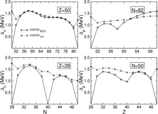
Figure 1: Comparison of the average pairing gaps calculated with a simple BCS, and the Lipkin-Nogami plus BCS approximations. For the $Z=50$ and $Z=28$ isotopes the neutron pairing gaps are shown, whereas for the $N=50$ and $N=82$ isotones the proton average pairing gaps are compared.

The intrinsic wave functions that will be used in configuration mixing calculations are obtained as solutions of the self-consistent RMF+LNBCS equations, subject to constraint on the mass quadrupole moment. As in the first part of this analysis NVR.06 , we use the relativistic point-coupling interaction PC-F1 BMM.02 in the particle-hole channel, and a density-independent $\delta$-force is the effective interaction in the particle-particle channel. The parameters of the PC-F1 interaction and the pairing strength constants $V_{n}$ and $V_{p}$ have been adjusted simultaneously to the nuclear matter equation of state, and to ground-state observables (binding energies, charge and diffraction radii, surface thickness and pairing gaps) of spherical nuclei BMM.02 , with pairing correlations treated in the BCS approximation. However, since the present analysis includes the LN approximate particle number projection, the pairing strength parameters have to be readjusted. By comparing the projected average pairing gaps $\langle uv\Delta\rangle^{(LN)}_{\tau}$ and the BCS pairing gaps $\langle uv\Delta\rangle^{(BCS)}_{\tau}$, we find that the neutron pairing strength should be reduced from $V_{n}=-308$ MeV to $V_{n}=-285$ MeV, and the proton pairing strength from $V_{p}=-321$ MeV to $V_{p}=-260$ MeV. The average pairing gaps for two isotopic and two isotonic chains are shown in Fig. 1. We notice that by readjusting the strength parameters $V_{n}$ and $V_{p}$, a good agreement between projected average pairing gaps and the BCS average pairing gaps is obtained except, of course, for magic numbers of neutrons or protons, for which an unphysical collapse of pairing correlations is found in the BCS approximation.

In order to illustrate the importance of including particle-number projection in the description of specific structure effects, we will compare the results of GCM calculations with those obtained using the model that was developed in the first part of this work NVR.06 , and in which the intrinsic wave functions are generated from the solutions of the constrained relativistic mean-field + BCS equations, without the Lipkin-Nogami approximate particle-number projection. In that case the correct mean-values of the nucleon numbers are restored by modifying the Hill-Wheller equations to include linear constraints on the number of protons and neutrons (see Eqs. (54) and (55) of Ref. NVR.06 ). Therefore, in the following subsections AMP will indicate that only angular momentum projection has been carried out before GCM configuration mixing (i.e. the model of Ref. NVR.06 is used), and PN&AMP will denote the results of GCM calculations which include both the restoration of the particle number and rotational symmetry.

In this section illustrative configuration mixing calculations are presented for ²⁴Mg, ³²S and ³⁶Ar. We choose these nuclei because the results can be directly compared with extensive GCM studies performed using the nonrelativistic Skyrme and Gogny effective interactions. In the analyses in which the nonrelativistic zero-range Skyrme interaction was used VHB.00 ; BFH.03 , both particle number and angular momentum projections were performed. The simultaneous projection on particle number and angular momentum is computationally much more demanding in the case of a finite-range interaction, and therefore only angular momentum projection was performed in the studies with the Gogny force RER.00 ; RER.02b ; RER.04 . Both approaches are interesting for the present analysis, because by comparing the results one can deduce which effects can be attributed to particle number projection, and which originate from the differences in the properties of the effective interactions.

The constrained RMF equations are solved by expanding the Dirac single-nucleon spinors in terms of eigenfunctions of an axially symmetric harmonic oscillator potential. In order to keep the basis closed under rotations, the two oscillator length parameters $b_{\perp}$ and $b_{z}$ have always identical values Rob.94 ; ERS.93 . In addition, to avoid the completeness problem in subsequent configuration mixing calculations, the same oscillator length is used for all values of the quadrupole deformations ERS.93 . Since we consider relatively light nuclei in this work, it is sufficient to use ten oscillator shells in the expansion (see Ref. NVR.06 for details).

III.1 ²⁴Mg

The low-energy spectrum of ²⁴Mg displays a typical rotational structure, with data on the ground-state band extending up to angular momentum $I=8\hbar$ Endt.90 ; EBF.98 . The spectroscopic quadrupole moment of the $2_{1}^{+}$ state: $-16.6(6)$ e fm² EBF.98 , indicates a large prolate deformation. The $0_{2}^{+}$ state is found at high excitation energy ($6.432$ MeV), and this means that shape-coexistence effects should only play a minor role in the description of the ground-state band. Properties of ²⁴Mg have been studied with the GCM using the Skyrme SLy4 VHB.00 , and the Gogny D1S RER.02b effective interactions.

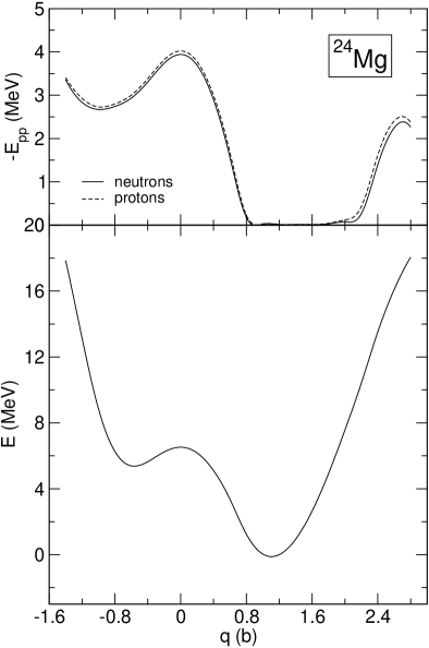
Figure 2: The BCS pairing energy for protons and neutrons (upper panel), and the mean-field plus BCS binding energy curve (lower panel) of ²⁴Mg, as functions of the mass quadrupole moment.

In Fig. 2 we display the pairing energy (upper panel), and the total RMF binding energy curve (lower panel) of ²⁴Mg, as functions of the mass quadrupole moment. The Lipkin-Nogami procedure has not been implemented at this stage, and consequently pairing correlations vanish in a broad region of deformations around the deformed first minimum of the potential energy surface. Since the moment of inertia of a rotational band is reduced in the presence of pairing correlations, dynamical pairing effects could be important in the description of the ground-state band of ²⁴Mg.

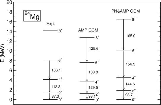
Figure 3: The ground-state rotational band in ²⁴Mg. The B(E2) values are in units of $e^{2}fm^{4}$. The GCM spectra calculated with (PN&AMP), and without (AMP) particle number projection, are compared with the experimental ground-state band Endt.90

The GCM excitation energies and the resulting transition probabilities for the ground-state band, calculated with the PC-F1 effective interaction, are shown in Fig. 3. The results of the AMP and PN&AMP configuration mixing calculations are compared with the data. As expected, the inclusion of dynamical pairing effects reduces the moment of inertia, but the resulting spectrum is much too spread out compared to experiment. This is a well known problem, related to the fact that we project particle number and angular momentum only after variation, rather than performing the projections before variation VS.71 . It has been shown that in the latter case rotational bands with larger moments of inertia are obtained HHR.82 ; SG.87 , provided that the model geometry allows for the alignment of nucleon angular momenta. Since the full projection before variation is technically and computationally much more complex, it has been seldom used in realistic calculations. We note that one possible improvement of the present model would be to project, for each value of the angular momentum $J$, the cranked mean-field wave functions which, in addition to the mass quadrupole moment, are also constrained to have $\langle J_{x}\rangle=J$ RS.80 ; BH.84 . This extension has not been included in the present analysis.

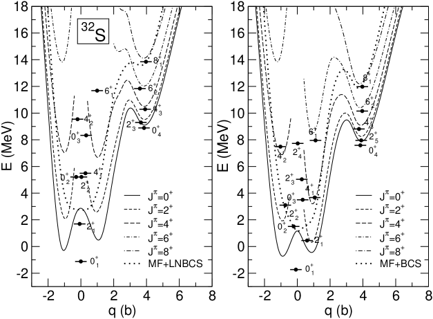
Figure 6: The energies and the average quadrupole moments of the GCM states in ³²S, plotted together with the corresponding angular momentum projected energy curves. GCM calculations with (left panel), and without (right panel) particle number projection are compared. The mean-field binding energy curves are also included in the figure (dotted curves). In both panels zero energy corresponds to the minimum of the $J=0$ projected energy curve.

The transition probabilities, as well as the calculated spectroscopic quadrupole moment $Q_{spec}(2_{1}^{+})=-16.56$ e fm², are in very good agreement with the data. The AMP GCM results are very similar to those obtained by using the Gogny D1S force (see Figs. 11 and 13 in Ref. RER.02b ), whereas the PN&AMP spectrum is close to the one calculated with the Skyrme SLy4 interaction (see Fig. 6 in Ref. VHB.00 ).

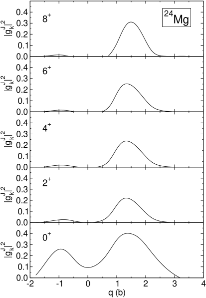
Figure 4: The amplitudes of the PN&AMP GCM collective wave functions $|g_{k}^{J}|^{2}$ of the ground-state band in ²⁴Mg.

The amplitudes of the PN&AMP GCM collective wave functions $|g_{k}^{J}|^{2}$ of the ground-state band, are plotted in Fig. 4 as functions of the mass quadrupole moment. It is interesting to note that only the $0_{1}^{+}$ state contains significant admixtures of oblate deformed shapes, whereas the amplitudes of states with $J\geq 2$ are concentrated in the prolate well. The same result has also been obtained with the Skyrme SLy4 interaction (see Fig. 4 of Ref. VHB.00 ).

III.2 ³²S

In recent years a number of theoretical and experimental studies of the structure of ³²S have been reported. This nucleus is particularly interesting because the excitation energies of the low-lying $0_{2}^{+}$, $2_{1}^{+}$ and $4_{1}^{+}$ states correspond to those of a typical spherical vibrator, whereas on the other hand, the quadrupole moment of the first $2^{+}$ state is large and negative, indicating large dynamical prolate deformation Rag.89 . ³²S is among the best studied nuclei in the $sd$ shell, and both the energies and lifetimes of many states up to $\approx 10$ MeV excitation energy are known Kan.98 ; BHM.02 .

Several modern theoretical approaches have been used in recent studies of normally deformed (ND), and superdeformed (SD) configurations in ³²S: the shell model with the universal sd-shell Hamiltonian Bre.97 , the semimicroscopic algebraic cluster model CLV.98 , and various extensions of the self-consistent mean-field framework. They include the cranked Hartree-Fock MDD.00 ; YM.00 ; TNI.01 , and Hartree-Fock-Bogoliubov method RER.00 for the description of the SD configuration, and the generator coordinate method with the Skyrme SLy6 BFH.03 , and Gogny D1S effective interactions, in the analysis of both ND and SD configurations RER.00 ; BFH.03 .

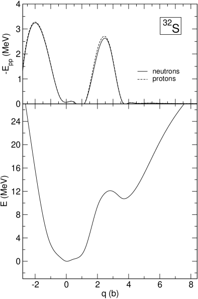
Figure 5: The BCS pairing energy for protons and neutrons (upper panel), and the mean-field plus BCS binding energy curve (lower panel) of ³²S, as functions of the mass quadrupole moment.

In Fig. 5 the pairing energy (upper panel), and the total RMF binding energy curve (lower panel) of ³²S, are plotted as functions of the mass quadrupole moment. The effective interaction is PC-F1, and pairing correlations are treated in the BCS approximation, without particle number projection. Consequently, we notice the collapse of the pairing energy both in the ND and the SD minima. This means that restoring the particle number symmetry could have an important effect in the description of both ground-state and SD bands.

The results of the PN&AMP and AMP GCM calculations for ³²S are shown in the left and right panels of Fig. 6, respectively. In the left (right) panel we also include the mean-field MF+LNBCS (MF+BCS) binding energy curve (dotted curves). In both cases the MF energy curve displays a spherical minimum, and an additional shallow minimum at large deformation $q\approx 4$b with excitation energy $E_{x}\approx 11$ MeV. The occurrence of almost degenerate oblate and prolate minima in the $J=0^{+}$ projected energy curve, symmetrical with respect to the spherical configuration, is a feature common to all nuclei for which the mean-field calculation predicts a spherical ground state (see, for instance, Refs. BFH.03 ; ER.04 ).

The superdeformed minimum is more pronounced in the calculation without particle number projection, both for the MF+BCS curve and for the angular momentum projected energy curves. The GCM superdeformed band is calculated at somewhat lower excitation energies in the AMP case, and this is because in the PN&AMP calculation pairing correlations do not vanish in the SD minimum. The energies of the GCM states are plotted as functions of the average quadrupole moment

$$q=\langle q_{k}\rangle=\sum_{j}{g_{k}^{2}(q_{j})q_{j}}\;.$$ (53)

The overall structure of energy levels, and in particular the two-phonon triplet $0_{2}^{+}$, $2_{2}^{+}$, $4_{1}^{+}$, is much better described when particle number projection is included (see Tables 1 and 2 for a comparison with experimental levels). Similar results for the spectra of ³²S have also been obtained in the GCM analyses of Refs. BFH.03 ; RER.00 . The calculation with the zero-range SLy6 effective interaction, including particle number projection, reproduces the structure of the two-phonon triplet BFH.03 . On the other hand, the results for the ND states obtained with the finite-range Gogny force, but with only angular momentum projection RER.00 , are similar to those shown in the right panel of Fig. 6, i.e. an additional low-lying $0^{+}$ state is predicted by the calculation.

In Tab. 1 we list the PN&AMP GCM excitation energies, the spectroscopic quadrupole moments, and the E2 (J $\to$ J -2) transition probabilities for the $2_{1}^{+}$ state, and for the two-phonon triplet $0_{2}^{+}$, $2_{2}^{+}$, $4_{1}^{+}$, in comparison with the results of Ref. BFH.03 , and the available data. The results obtained with both effective interactions, the nonrelativistic SLy6 and the relativistic PC-F1, are in qualitative agreement with the data. The excitation energies of the two-phonon triplet are calculated at approximately twice the energy of the $2_{1}^{+}$ state. We note, however, that the predicted quadrupole moments for the $2_{1}^{+}$ state are small and positive, whereas the experimental value points to a much larger and prolate deformation of this state.

A small prolate deformation for the ground-state band is only obtained in calculations which do not include particle number projection (right panel of Fig. 6). In Tab. 2 we compare the AMP GCM excitation energies and B(E2, J $\to$ J -2) values obtained with PC-F1, with the corresponding quantities calculated with the Gogny D1S interaction RER.00 . The results are very similar, with the largest differences in the B(E2) values for the transitions $2_{1}^{+}\to 0_{1}^{+}$ and $2_{2}^{+}\to 0_{3}^{+}$. This can be attributed to the smaller values of the quadrupole moments of the $2^{+}$ states predicted by the PC-F1 interaction. For instance, the spectroscopic quadrupole moment of the $2_{1}^{+}$ state calculated with the Gogny force $-13.29$ e fm² is close to the experimental value: $-14.9$ e fm² Endt.90 , whereas the one predicted by the PC-F1 interaction: $-3.5$ e fm², is much too small.

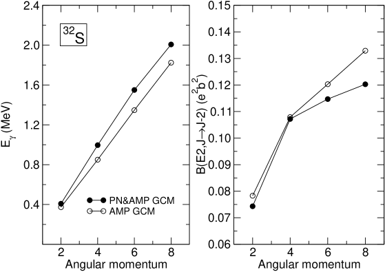
Figure 7: Transition energies $\Delta E(J)=E(J)-E(J-2)$ (left panel), and the B(E2, J$\to$ J-2) values (right panel), for the SD configuration in ³²S, as functions of the angular momentum.

Although the present version of the RMF plus GCM model is not optimal for the study of moments of inertia of superdeformed rotational bands, because it does not include cranked wave functions, nevertheless it can be used to investigate the stability of the SD intrinsic configurations against quadrupole fluctuations at low angular momentum. In Fig. 6 it is shown that both the PN&AMP and AMP GCM calculations predict an SD band at large deformation $q\approx 4b$. In the left panel of Fig. 7 we plot the energy differences $\Delta E(J)=E(J)-E(J-2)$, as functions of the angular momentum of the SD band. Since without particle number projection pairing correlations vanish in the SD minimum, the AMP GCM calculation overestimates the moment of inertia of the SD band, and the resulting spectrum is more compressed. The moment of inertia is reduced with the inclusion of dynamical pairing effects. In the right panel of Fig. 7 we include the corresponding E2 transition probabilities. Both the relative excitation energies and the B(E2) values for the SD band are consistent with the results reported in Ref. BFH.03 (Tab. VIII), and Ref. RER.00 (Fig. 3). We note, however, differences in the predicted position of the SD band-head. In our PN&AMP GCM calculation the SD band-head is found at $8.9$ MeV, almost $3$ MeV lower than the value calculated with the SLy6 interaction in Ref. BFH.03 . The AMP GCM calculation predicts the head of the SD band at $7.6$ MeV, comparable to the value obtained with the Gogny D1S interaction in Ref. RER.00 ($8.9$ MeV). A possible reason for the large difference between the PC-F1 and Gogny D1S interactions on one hand, and the SLy6 Skyrme force on the other, can be identified already at the mean-field level. While the energy curves obtained with the PC-F1 and Gogny interactions (see also Fig. 2 in Ref. RER.00 ) exhibit a second, superdeformed shallow minimum at $q\approx 4b$, only a shoulder in the potential energy curve at superdeformation is predicted by the SLy6 interaction (see Fig. 13 in Ref. BFH.03 ).

III.3 ³⁶Ar

In the last example we present the GCM analysis of the low angular momentum structure of ³⁶Ar, one of the lightest nuclei in which a superdeformed structure has been studied experimentally. The excitation energies and $E2$ transition probabilities for the prolate SD band have been recently measured up to the angular momentum $I=16\hbar$ Sve.00 . The properties of the oblate ground-state band were determined over a decade ago Endt.90 . A number of theoretical analyses of the structure of ³⁶Ar include the cranked Nilsson-Strutinsky and the shell model Sve.00 ; Sve.01 , the projected shell model LS.01 , the self-consistent cranked Hartree-Fock-Bogoliubov model RER.04 , and the generator coordinate method with Skyrme SLy6 BFH.03 and Gogny D1S RER.04 interactions.

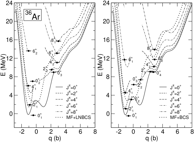
Figure 8: The energies and the average quadrupole moments of the GCM states in ³⁶Ar, plotted together with the corresponding angular momentum projected energy curves. GCM calculations with (left panel), and without (right panel) particle number projection are compared. The mean-field binding energy curves are also included in the figure (dotted curves). In both panels zero energy corresponds to the minimum of the $J=0$ projected energy curve.

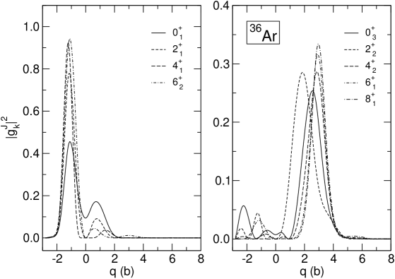
Figure 10: The amplitudes of the PN&AMP GCM collective wave functions $|g_{k}^{J}|^{2}$ for the ND ground-state band ($0_{1}^{+}$, $2_{1}^{+}$, $4_{1}^{+}$ and $6_{2}^{+}$), and the SD band ($0_{3}^{+}$, $2_{2}^{+}$, $4_{2}^{+}$ and $6_{1}^{+}$ and $8_{1}^{+}$) in ³⁶Ar, as functions of the mass quadrupole moment.

The results of the PN&AMP and the AMP GCM calculations are shown in the left and right panels of Fig. 8, respectively. In both cases the mean-field binding energy curve is also included (dotted curves). The BCS mean-field energy curve displays an oblate minimum, rather flat in the region of deformation: $-1$ b $\leq$ q $\leq 0.5$ b. In addition, a shallow minimum is found at larger deformation $q\approx 2.8$ b, at $E_{x}\approx 9$ MeV above the ground-state minimum, and a shoulder is predicted at still larger deformation $q\approx 5$ b. A similar mean-field potential energy surface is obtained with the Gogny D1S interaction (see Fig. 1 in Ref. RER.04 ), but the SD minimum is calculated $\approx 1$ MeV lower than with PC-F1. We note that in the BCS approximation pairing correlations vanish both in the ND and SD minimum, and this means that the restoration of particle number can produce sizable effects in the ground-state and SD bands. The mean-field energy curve which includes the approximate particle number projection (LNBCS), displays only a weak shoulder, rather than a minimum at deformation $q\approx 3$ b. This curve is in qualitative agreement with the LNBCS binding energy curve calculated with the Skyrme SLy6 effective interaction (see Fig. 10 in Ref. BFH.03 ), although in the latter case the shoulder occurs at smaller deformation $q\approx 1.8$ b, and much smaller excitation energy $E_{x}\approx 5$ MeV. Both in the PN&AMP and the AMP calculations, the $J=0$ angular momentum projected energy curves display two well developed low-lying minima on the oblate and prolate side. The oblate minimum corresponds to the ground state. An additional SD minimum occurs on the AMP $J=0$ energy curve, whereas the corresponding PN&AMP curve displays only a plateau. The angular momentum projected energy curves with $J\geq 2$ exhibit well developed SD minima both in the AMP and PN&AMP calculations. Finally, the energies of the resulting GCM states for angular momenta $J\leq 8$ are included as functions of the average quadrupole moment, defined in Eq. (53). The low-spin GCM spectra contain an oblate ND ground state band, and a prolate SD band.

In Tab. 3 we compare the PN&AMP GCM excitation energies, the spectroscopic quadrupole moments, and the B(E2, J $\to$ J-2) values for the ground-state band, with the results obtained with the Skyrme SLy6 interaction in Ref. BFH.03 , and with available data. The theoretical results are in qualitative agreement. Although the energy spectrum is described somewhat better by the PC-F1 interaction, both calculations clearly underestimate the moment of inertia of the ND ground-state band. In Tab. 4 the AMP GCM excitation energies and the B(E2, J $\to$ J-2) values for the ND band, are shown in comparison with those calculated with the Gogny D1S interaction in Ref. RER.04 . The results obtained with the PC-F1 and Gogny effective interactions are very similar, and a considerable increase of the moment of inertia as compared to the PN&AMP GCM spectra, is caused by the collapse of pairing correlations in the ND minimum.

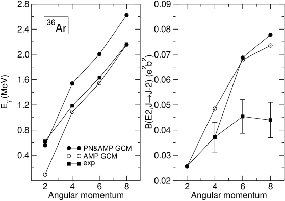
Figure 9: The energy differences $\Delta E(J)=E(J)-E(J-2)$ (left panel), and the B(E2, J$\to$ J-2) values (right panel), for the SD band in ³⁶Ar, as functions of the angular momentum. Results of GCM calculations with and without particle number projection are compared with the available data Sve.00 ; Sve.01 .

In the left panel of Fig. 9 we plot the energy differences $\Delta E(J)=E(J)-E(J-2)$, and in the right panel the $BE2$ values, as functions of the angular momentum of the SD band, in comparison with data. Cranked Hartree-Fock-Bogoliubov calculations performed with the Gogny interaction RER.04 , have shown that rather strong triaxiality effects appear already at zero-spin and, as a result, predicted a steady decrease of deformation with increasing angular momentum. Being restricted to axially symmetric shapes, the model that we have developed in this work cannot take these effects into account. This is clearly reflected in the pronounced discrepancy between the calculated and experimental B(E2) values. Similar results have also been obtained with the SLy6 (see Tab. V in Ref. BFH.03 ), and Gogny effective interactions (see Fig. 3 in Ref. RER.04 ). Just like in the case of ³²S that we have considered in the previous section, the transition energies and the B(E2) values do not crucially depend on the effective interaction in the particle-hole channel. On the other hand, the predicted positions of the SD band-head differ significantly: for the Gogny D1S interaction the band-head is at $7.5$ MeV, whereas the SLy6 interaction predicts a lower value of $5.9$ MeV. The positions of SD band-head obtained in the PN&AMP and AMP GCM calculations with the PC-F1 interaction are $9.2$ MeV and $9.4$ MeV, respectively.

Finally, the amplitudes of the collective PN&AMP GCM wave functions $|g_{k}^{J}|^{2}$ for the ND ($0_{1}^{+}$, $2_{1}^{+}$, $4_{1}^{+}$ and $6_{2}^{+}$), and the SD ($0_{3}^{+}$, $2_{2}^{+}$, $4_{2}^{+}$ and $6_{1}^{+}$ and $8_{1}^{+}$) rotational bands in ³⁶Ar are plotted in Fig. 10. We notice that, except for the ground state $0_{1}^{+}$, the amplitudes of the states of the ND band are principally concentrated in the oblate minimum, whereas in the panel on the right the amplitudes of the wave functions are strongly peaked in the prolate superdeformed minimum.

IV Summary and outlook

In Ref. NVR.06 and in this work we have extended the very successful relativistic mean-field theory BHR.03 ; VALR.05 to explicitly include correlations related to the restoration of broken symmetries and to fluctuations of collective coordinates. We have developed a model that uses the generator coordinate method to perform configuration mixing of angular-momentum and particle-number projected relativistic wave functions. The geometry is restricted to axially symmetric shapes, and the intrinsic wave functions are generated from the solutions of the relativistic mean-field + Lipkin-Nogami BCS equations, with a constraint on the mass quadrupole moment. The single-nucleon Dirac eigenvalue equation is solved by expanding the large and small components of the nucleon spinor in terms of eigenfunctions of an axially symmetric harmonic oscillator potential. The current implementation of the model employs a relativistic point-coupling (contact) nucleon-nucleon effective interaction in the particle-hole channel, and a density-independent $\delta$-interaction in the particle-particle channel.

We have performed several illustrative calculations which test our implementation of the GCM with simultaneous particle-number and angular-momentum projection. The results have been compared with those obtained employing the relativistic GCM model developed in the first part of this work NVR.06 , which does not include particle-number projection, but only conserves the number of particles on the average, and with results that were obtained using the corresponding non-relativistic models based on Skyrme and Gogny effective interactions. In this work the low-lying spectra of ²⁴Mg, ³²S and ³⁶Ar have been analyzed. The results of GCM configuration mixing calculations both without and with particle-number projection, have been compared with those obtained with the angular-momentum projected GCM based on the Gogny D1S effective interaction, and with the particle-number and angular-momentum projected GCM based on the Skyrme SLy4 and SLy6 effective interactions. The principal features of the spectra calculated without (Gogny interaction) and with particle-number projection (Skyrme forces), are very well reproduced in our GCM calculation with the PC-F1 relativistic effective interaction. These include the deformations and moments of inertia of yrast bands, and the occurrence and structure of superdeformed bands. Some differences between the predictions of the three models, as for instance the position of the head $0^{+}$ of the superdeformed band, can be attributed to the gaps in the mean-field single-nucleon spectra calculated with the different effective interactions. We have also shown that dynamical pairing effects play an important role in the description of the low-energy spectra. In particular, we find a pronounced effect of particle-number projection on the moments of inertia of the ground-state and superdeformed rotational bands. Another example is the two-phonon triplet $0_{2}^{+}$, $2_{2}^{+}$ and $4_{1}^{+}$ in ³²S, which can be reproduced by GCM calculations only when dynamical pairing effects are taken into account.

There are, of course, many possible improvements and extensions of the present implementation of the relativistic GCM model. Perhaps the most obvious is the extension to shapes that are not constrained by axial symmetry. The inclusion of triaxial deformations is in principle straightforward but, because it requires an enormous increase of computational capabilities, not feasible at present. The second major problem is that our GCM configuration mixing calculations correspond to a projection after variation. A more general variation after projection is far too complicated to be used in realistic calculations at the present stage. A possible improvement, however, is to generate the GCM basis functions, for each value of the angular momentum, by performing cranking RMF+LNBCS calculations with the additional constraint $\langle J_{x}\rangle=\sqrt{J(J+1)}$. This would automatically increase the moments of inertia of rotational bands, and therefore produce spectra in better agreement with experiment. The extension to odd-A nuclei necessitates the breaking of time-reversal invariance in the wave functions and, therefore, the explicit inclusion of currents in the energy-density functional, and the corresponding time-odd fields in the single-nucleon Dirac equation. Finally, let us emphasize again one the conclusions of Ref. NVR.06 , namely that those correlations which are explicitly treated in the GCM configuration mixing, should not be contained in the effective interaction in an implicit way, i.e. by adjusting the parameters of the interaction to data which already include these correlations. Therefore, before the present version of the relativistic self-consistent GCM is applied in realistic calculations, we need to adjust a new global effective interaction which will not contain symmetry breaking corrections and quadrupole fluctuation correlations. *

Appendix A Evaluation of the parameter $\lambda_{2}$ in the Lipkin-Nogami method

The variation of the auxiliary functional $\mathcal{K}$ Eq. (12) can be expressed as

$$\langle\mathcal{K}\hat{N}_{2}^{2}\rangle=0\;,$$ (54)

for the ground-state expectation value, with $\hat{N}_{2}$ as the two-quasiparticle part of the particle-number operator Eq. (17). Since we do not consider proton-neutron pairing, the equations for protons and neutrons separate, and the isospin index $q$ can be omitted in the following derivation. If one introduces the shifted many-body state

$$\left|\xi\right\rangle=e^{i\xi\hat{N}_{2}}\left|0\right\rangle,\qquad\left|0\right\rangle=\left|\xi\right\rangle\Big{|}_{\xi=0}\;,$$ (55)

the following expression for $\lambda_{2}$ is obtained from the variational condition Eq. (54) RNB.96

$$\lambda_{2}=\frac{\partial_{\xi}^{2}\left\langle 0\right|\hat{H}\left|\xi\right\rangle\Big{|}_{\xi=0}}{\partial_{\xi}^{2}\left\langle 0\right|\hat{N}^{2}\left|\xi\right\rangle\Big{|}_{\xi=0}}\;.$$ (56)

The denominator of this equation is evaluated using Wick’s theorem

$$\partial_{\xi}^{2}\left\langle 0\right|\hat{N}^{2}\left|\xi\right\rangle\Big{|}_{\xi=0}=32\left[(\overline{u^{2}v^{2}})^{2}-\overline{u^{4}v^{4}}\right]\;.$$ (57)

The principal advantage of this particular formulation of the Lipkin-Nogami scheme is that one can relate it to the theoretical framework of energy density functionals RNB.96

$$\left\langle 0\right|\hat{H}\left|\xi\right\rangle\Longleftrightarrow\mathcal{E}^{(\xi)}=\mathcal{E}[\hat{\rho}^{(\xi)},\hat{\kappa}^{(\xi)},\hat{\kappa}^{*(\xi)}]\;,$$ (58)

with the following definition of the shifted densities

$$\rho_{kl}^{(\xi)}=\left\langle 0\right|a_{l}^{\dagger}a_{k}\left|\xi\right\rangle,\qquad\kappa_{kl}^{(\xi)}=\left\langle 0\right|a_{\bar{l}}a_{k}\left|\xi\right\rangle\;.$$ (59)

The second derivative of the energy functional reads

$$\partial_{\xi}^{2}\mathcal{E}^{(\xi)} = {\rm Tr}\left[\frac{\delta\mathcal{E}}{\delta\hat{\rho}}\partial_{\xi}^{2}\hat{\rho}+\frac{\delta\mathcal{E}}{\delta\hat{\kappa}}\partial_{\xi}^{2}\hat{\kappa}+\frac{\delta\mathcal{E}}{\delta\hat{\kappa}^{*}}\partial_{\xi}^{2}\hat{\kappa}^{*}\right]$$ (60)

$$+ 2{\rm Tr}~{}{\rm Tr}\left[\frac{1}{2}\frac{\delta^{2}\mathcal{E}}{\delta\hat{\rho}_{1}\delta\hat{\rho}_{2}}\partial_{\xi}\hat{\rho}_{1}\partial_{\xi}\hat{\rho}_{2}+\frac{\delta^{2}\mathcal{E}}{\delta\hat{\kappa}\delta\hat{\kappa}^{*}}\partial_{\xi}\hat{\kappa}\partial_{\xi}\hat{\kappa}^{*}+\frac{\delta^{2}\mathcal{E}}{\delta\hat{\rho}\delta\hat{\kappa}}\partial_{\xi}\hat{\rho}\partial_{\xi}\hat{\kappa}+\frac{\delta^{2}\mathcal{E}}{\delta\hat{\rho}\delta\hat{\kappa}^{*}}\partial_{\xi}\hat{\rho}\partial_{\xi}\hat{\kappa}^{*}\right]\;$$

where the trace implies integration and summation over all coordinates. The term with a single trace vanishes in the BCS ground state RNB.96 and, since we use volume pairing in the energy functional (see Eq. 9), the mixed derivative terms which contain $\hat{\rho}$ and $\hat{\kappa}$, or $\hat{\rho}$ and $\hat{\kappa}^{*}$, also vanish. With the definition of the response densities $\tilde{\rho}$, $\tilde{\kappa}$ and $\tilde{\kappa}^{*}$

$$\tilde{\rho}=-i\partial_{\xi}\hat{\rho}^{(\xi)}\Big{|}_{\xi=0},\quad\tilde{\kappa}=-i\partial_{\xi}\hat{\kappa}^{(\xi)}\Big{|}_{\xi=0}\quad{\textrm{and}}\quad\tilde{\kappa}^{*}=-i\partial_{\xi}\hat{\kappa}^{(\xi)*}\Big{|}_{\xi=0}\;,$$ (61)

one finally obtains

$$\partial_{\xi}^{2}\mathcal{E}^{(\xi)}=-{\rm Tr}~{}{\rm Tr}\left[\frac{\delta^{2}\mathcal{E}}{\delta\hat{\rho}_{1}\delta\hat{\rho}_{2}}\tilde{\rho}_{1}\tilde{\rho}_{2}+2\frac{\delta^{2}\mathcal{E}}{\delta\hat{\kappa}\delta\hat{\kappa}^{*}}\tilde{\kappa}\tilde{\kappa}^{*}\right]\;.$$ (62)

The RMF energy functional considered in this work consists of three terms:
i) the kinetic energy

$$\mathcal{E}_{kin}=\sum_{k}{\int d\bm{r}~{}v_{k}^{2}~{}{\bar{\psi}_{k}(\bm{r})\left(-i\bm{\gamma}\bm{\nabla}+m\right)\psi_{k}(\bm{r})}}\;,$$ (63)

ii) the field energy

$$\mathcal{E}_{field} = \int d{\bm{r}}~{}{\left(\frac{\alpha_{S}}{2}\rho_{S}^{2}+\frac{\beta_{S}}{3}\rho_{S}^{3}+\frac{\gamma_{S}}{4}\rho_{S}^{4}+\frac{\delta_{S}}{2}\rho_{S}\triangle\rho_{S}+\frac{\alpha_{V}}{2}j_{\mu}j^{\mu}+\frac{\gamma_{V}}{4}(j_{\mu}j^{\mu})^{2}+\frac{\delta_{V}}{2}j_{\mu}\triangle j^{\mu}\right.}$$ (64)

$$+ \left.\frac{\alpha_{TV}}{2}j^{\mu}_{TV}(j_{TV})_{\mu}+\frac{\delta_{TV}}{2}j^{\mu}_{TV}\triangle(j_{TV})_{\mu}+\frac{\alpha_{TS}}{2}\rho_{TS}^{2}+\frac{\delta_{TS}}{2}\rho_{TS}\triangle\rho_{TS}\right)\;,$$

and iii) the Coulomb interaction term

$$\mathcal{E}_{C}=\frac{e^{2}}{2}\int\int d{\bm{r}}d{\bm{r}^{\prime}}\frac{\rho_{p}(\bm{r})\rho_{p}(\bm{r}^{\prime})}{|\bm{r}-\bm{r^{\prime}}|^{2}}\;.$$ (65)

The response densities which appear in Eq. (62) are given by

$$\rho_{S}^{\tau}(\bm{r}) = \sum_{k}u_{k}^{2}v_{k}^{2}\bar{\psi}_{k}(\bm{r})\psi_{k}(\bm{r})$$ (66)

$$j_{\mu}^{\tau}(\bm{r}) = \sum_{k}u_{k}^{2}v_{k}^{2}\bar{\psi}_{k}(\bm{r})\gamma_{\mu}\psi_{k}(\bm{r})\;,$$ (67)

where the summation runs for $\tau=n(p)$ over neutron (proton) single-particle states. The functional derivative of $\mathcal{E}_{field}$ reads

$$\partial_{\xi}^{2}\mathcal{E}^{(\xi)\tau}_{field} = \int d\bm{r}\left[(\alpha_{S}+2\beta_{S}\rho_{S}+3\gamma_{S}\rho_{S}^{2}+\alpha_{TS})\tilde{\rho_{S}}^{\tau}\tilde{\rho_{S}}^{\tau}+(\delta_{S}+\delta_{TS})\tilde{\rho_{S}}^{\tau}\triangle\tilde{\rho_{S}}^{\tau}\right.$$ (68)

$$+ \left.(\alpha_{V}+3\gamma_{S}j_{\mu}j^{\mu}+\alpha_{TV})\tilde{j}_{\nu}^{\tau}\tilde{j}^{\nu\tau}+(\delta_{V}+\delta_{TV})\tilde{j}_{\nu}^{\tau}\triangle\tilde{j}^{\nu\tau}\right]\;,$$

where $\rho_{S}$ and $j_{\mu}$ denote the scalar density and baryon current, respectively , and $\rho_{S}^{\tau}$ and $j_{\mu}^{\tau}$ are the corresponding neutron (proton) densities and currents. For protons there is an additional contribution from the Coulomb interaction:

$$\partial_{\xi}^{2}\mathcal{E}^{(\xi)}_{C}=e^{2}\int\int d{\bm{r}}d{\bm{r}^{\prime}}\frac{\tilde{\rho}^{p}(\bm{r})\tilde{\rho}^{p}(\bm{r}^{\prime})}{|\bm{r}-\bm{r^{\prime}}|^{2}}\;.$$ (69)

To evaluate the contribution of the pairing energy Eq. (9) to the second derivative of the energy functional, one needs the non-hermitian response pairing tensor

$$\tilde{\kappa}^{\tau}(\bm{r}) = -4\sum_{k>0}f_{k}^{2}u_{k}^{3}v_{k}\psi^{\dagger}_{k}(\bm{r})\psi_{k}(\bm{r})$$ (70)

$$\tilde{\kappa}^{\tau*}(\bm{r}) = 4\sum_{k>0}f_{k}^{2}u_{k}v_{k}^{3}\psi^{\dagger}_{k}(\bm{r})\psi_{k}(\bm{r})\;.$$ (71)

This leads to a rather simple expression

$$\partial_{\xi}^{2}\mathcal{E}^{(\xi)\tau}_{pair}=\frac{V_{q}}{2}\int d\bm{r}\tilde{\kappa}^{\tau}\tilde{\kappa}^{\tau*}\;.$$ (72)

Finally, by inserting Eqs. (68), (69), and (72) into Eq. (56), one obtains the Lipkin-Nogami parameter $\lambda_{2,\tau}$.

ACKNOWLEDGMENTS

This work has been supported in part by the Bundesministerium für Bildung und Forschung - project 06 MT 246, by the Gesellschaft für Schwerionenforschung GSI - project TM-RIN, and by the Alexander von Humboldt Stiftung.

Table 1: Excitation energies, spectroscopic quadrupole moments and B(E2, J $\to$ J-2) values for the one-phonon ($2_{1}^{+}$) state, and the two-phonon triplet ($0_{2}^{+}$, $2_{2}^{+}$ and $4_{1}^{+}$) in ³²S. GCM calculations performed with particle number projection are compared with the results reported in Ref. BFH.03 , and with available data.

state	$E_{x}$ (MeV)			$Q_{spec}(efm^{2})$			Transition	$BE2(e^{2}fm^{4})$
	This work	Ref. BFH.03	Exp.	This work	Ref. BFH.03	Exp.		This work	Ref. BFH.03	Exp.
$0_{1}^{+}$	0.0	0.0	0.0	-	-	-	-	-	-	-
$2_{1}^{+}$	2.81	3.22	2.23	5.8	2.3	-14.9	$2_{1}^{+}\to 0_{1}^{+}$	94	38	61
$0_{2}^{+}$	6.33	6.32	3.78	-	-	-	$0_{2}^{+}\to 2_{1}^{+}$	37	144	72
$2_{2}^{+}$	6.33	7.04	4.28	-3.0	-0.7	-	$2_{2}^{+}\to 2_{1}^{+}$	131	157	54
						-	$2_{2}^{+}\to 0_{1}^{+}$	0.134	0.02	11
						-	$2_{2}^{+}\to 0_{2}^{+}$	10.7	2.8	-
$4_{1}^{+}$	6.61	7.35	4.46	-1.2	11.7	-	$4_{1}^{+}\to 2_{1}^{+}$	140.5	94	72

Table 2: Excitation energies and B(E2, J $\to$ J-2) values for the two lowest bands in ³²S. The results of GCM calculations performed without particle number projection are shown in comparison with those of Ref. RER.00 .

state	$E_{x}$ (MeV)		Transition	$BE2(e^{2}fm^{4})$
	This work	Ref. RER.00		This work	Ref. RER.00
$0_{1}^{+}$	0.0	0.0	-	-	-
$2_{1}^{+}$	2.181	2.107	$2_{1}^{+}\to 0_{1}^{+}$	66.2	72.3
$4_{1}^{+}$	5.395	5.825	$4_{1}^{+}\to 2_{1}^{+}$	102.9	119.8
$6_{1}^{+}$	9.661	10.962	$6_{1}^{+}\to 4_{1}^{+}$	146.1	142.8
$0_{3}^{+}$	3.24	3.778	-	-	-
$2_{2}^{+}$	4.832	4.282	$2_{2}^{+}\to 0_{3}^{+}$	33.3	58.0
$4_{2}^{+}$	9.213	9.097	$4_{2}^{+}\to 2_{2}^{+}$	121.1	132.2

Table 3: Excitation energies, spectroscopic quadrupole moments, and B(E2, J $\to$ J-2) values for the ground-state band in ³⁶Ar. GCM calculations performed with particle number projection are compared with those of Ref. BFH.03 , and with available data.

state	$E_{x}$ (MeV)			$Q_{spec}(efm^{2})$			Transition	$BE2(e^{2}fm^{4})$
	This work	Ref. BFH.03	Exp.	This work	Ref. BFH.03	Exp.		This work	Ref. BFH.03	Exp.
$0_{1}^{+}$	0.0	0.0	0.0	-	-	-	-	-	-	-
$2_{1}^{+}$	2.26	2.8	1.97	13	13	-	$2_{1}^{+}\to 0_{1}^{+}$	79	44	60$\pm$ 6
$4_{1}^{+}$	6.40	7.43	4.41	14	12	-	$4_{1}^{+}\to 2_{1}^{+}$	129	103	-
$6_{2}^{+}$	13.94	13.65	9.18	9.9	-1.3	-	$6_{2}^{+}\to 4_{1}^{+}$	152	93	-

Table 4: Excitation energies and B(E2, J $\to$ J-2) values for the ground-state band in ³⁶Ar. GCM calculations performed without particle number projection are compared with the results reported in Ref. RER.04 .

state	$E_{x}$ (MeV)		Transition	$BE2(e^{2}fm^{4})$
	This work	Ref. RER.04		This work	Ref. RER.04
$0_{1}^{+}$	0.0	0.0	-	-	-
$2_{1}^{+}$	1.54	1.45	$2_{1}^{+}\to 0_{1}^{+}$	74.8	72.1
$4_{1}^{+}$	4.99	4.54	$4_{1}^{+}\to 2_{1}^{+}$	114.7	102.3
$6_{1}^{+}$	12.15	10.01	$6_{1}^{+}\to 4_{1}^{+}$	142.4	112.8

References

- (1) T. Nikšić, D. Vretenar, and P. Ring, Phys. Rev. C73, 034308 (2006).
- (2) M. Bender, P.-H. Heenen, and P.-G. Reinhard, Rev. Mod. Phys. 75, 121 (2003).
- (3) D. Vretenar, A. V. Afanasjev, G. A. Lalazissis, and P. Ring, Physics Reports 409, 101 (2005).
- (4) T. Bürvenich, D. G. Madland, J. A. Maruhn, and P.-G. Reinhard, Phys. Rev. C65, 044308 (2002).
- (5) S. J. Krieger, P. Bonche, H. Flocard, P. Quentin, and M. S. Weiss, Nucl. Phys. A517, 275 (1990).
- (6) H. J. Lipkin, Ann. Phys. (N.Y.) 31, 525 (1960).
- (7) Y. Nogami, Phys. Rev. B134, 313 (1964).
- (8) H. Flocard and N. Onishi, Ann. Phys. (N.Y.) 254, 275 (1997).
- (9) A. Valor, J. L. Egido, and L. M. Robledo, Phys. Rev. C53, 172 (1996).
- (10) A. Valor, J. L. Egido, and L. M. Robledo, Phys. Lett B392, 249 (1997).
- (11) P.-G. Reinhard, W. Nazarewicz, M. Bender, and J. A. Maruhn, Phys. Rev. C53, 2776 (1996).
- (12) M. Bender, K. Rutz, P.-G. Reinhard, and J. A. Maruhn, Eur. Phys. J. A8, 59 (2000).
- (13) J. Dobaczewski, H. Flocard, and J. Treiner, Nucl. Phys. A422, 103 (1984).
- (14) S. Ćwiok, J. Dobaczewski, P.-H. Heenen, P. Magierski, and W. Nazarewicz, Nucl. Phys. A611, 211 (1996).
- (15) L. Bennour, P.-H. Heenen, P. Bonche, J. Dobaczewski, and H. Flocard, Phys. Rev. C40, 2834 (1989).
- (16) P. Quentin, N. Redon, J. Meyer, and M. Meyer, Phys. Rev. C41, 341 (1990).
- (17) Y. K. Gambhir, P. Ring, and A. Thimet, Ann. Phys. (N.Y.) 198, 132 (1990).
- (18) P. Ring and P. Schuck, The nuclear many-body problem (Springer, Heidelberg, 1980).
- (19) D. A. Varshalovich, A. N. Moskalev, and V. K. Khersonskii, Quantum theory of angular momentum (World Scientific Publishing Co., Inc., New Jersey, 1988).
- (20) D. L. Hill and J. A. Wheeler, Phys. Rev. 89, 1102 (1953).
- (21) N. Onishi and S. Yoshida, Nucl. Phys. 80, 267 (1966).
- (22) R. Balian and E. Brezin, Nuovo Cim. 64B, 37 (1969).
- (23) A. Valor, P.-H. Heenen, and P. Bonche, Nucl. Phys. A671, 145 (2000).
- (24) P. Bonche, J. Dobaczewski, H. Flocard, P.-H. Heenen, and J. Meyer, Nucl. Phys. A510, 466 (1990).
- (25) V. N. Fomenko, J. Phys. (GB) A3, 8 (1970).
- (26) M. Anguiano, J. L. Egido, and L. M. Robledo, Nucl. Phys. A696, 467 (2001).
- (27) L. F. F. Lathouvers, Ann. Phys. (N.Y.) 102, 347 (1976).
- (28) R. R. Rodríguez-Guzmán, J. L. Egido, and L. M. Robledo, Nucl. Phys. A709, 201 (2002).
- (29) M. Bender, H. Flocard, and P.-H. Heenen, Phys. Rev. C68, 044321 (2003).
- (30) R. R. Rodríguez-Guzmán, J. L. Egido, and L. M. Robledo, Phys. Lett. B474, 15 (2000).
- (31) R. R. Rodríguez-Guzmán, J. L. Egido, and L. M. Robledo, Phys. Rev. C69, 054319 (2004).
- (32) L. Robledo, Phys. Rev. C50, 2874 (1994).
- (33) J. L. Egido, L. M. Robledo, and Y. Sun, Nucl. Phys. A560, 253 (1993).
- (34) P. M. Endt, Nucl. Phys. A510, 1 (1990).
- (35) P. M. Endt, J. Blachot, R. B. Firestone, and J. Zipkin, Nucl. Phys. A633, 1 (1998).
- (36) F. Villars and N. Schmeing-Rogerson, Ann. Phys. (N.Y.) 63, 443 (1971).
- (37) K. Hara, A. Hayashi, and P. Ring, Nucl. Phys. A385, 14 (1982).
- (38) K. W. Schmid and F. Grümmer, Rep. Prog. Phys. 50, 731 (1987).
- (39) D. Baye and P.-H. Heenen, Phys. Rev. C29, 1056 (1984).
- (40) P. Raghavan, At. Data Nucl. Data Tables 42, 189 (1989).
- (41) A. Kangasmäki et al., Phys. Rev. C58, 699 (1998).
- (42) M. Babilon, T. Hartmann, P. Mohr, K. Vogt, S. Volz, and A. Zilges, Phys. Rev. C65, 037303 (2002).
- (43) J. Brenneisen et al., Z. Phys. A357, 377 (1997).
- (44) J. Cseh, G. Lévai, A. Ventura, and L. Zuffi, Phys. Rev. C58, 2144 (1998).
- (45) H. Molique, J. Dobaczewski, and J. Dudek, Phys. Rev. C61, 044304 (2000).
- (46) M. Yamagami and K. Matsuyanagi, Nucl. Phys. A672, 123 (2000).
- (47) T. Tanaka, R. G. Nazmitdinov, and K. Iwasawa, Phys. Rev. C63, 034309 (2001).
- (48) J. L. Egido and L. M. Robledo, in Lecture Notes in Physics, edited by G. Lalazissis, P. Ring, and D. Vretenar (Springer-Verlag, Heidelberg, 2004), Vol. 641, p. 269.
- (49) C. E. Svensson et al., Phys. Rev. Lett. 85, 2693 (2000).
- (50) C. E. Svensson et al., Phys. Rev. C63, 061301 (2001).
- (51) G.-L. Long and Y. Sun, Phys. Rev. C63, 021305 (2001).