Radial sensitivity of kaonic atoms and strongly bound $\bar{K}$ states

Abstract

The strength of the low energy $K^{-}$-nucleus real potential has recently received renewed attention in view of experimental evidence for the possible existence of strongly bound $K^{-}$ states. Previous fits to kaonic atom data led to either ‘shallow’ or to ‘deep’ potentials, where only the former are in agreement with chiral approaches but only the latter can produce strongly bound states. Here we explore the uncertainties of the $K^{-}$-nucleus optical potentials, obtained from fits to kaonic atom data, using the functional derivatives of the best-fit $\chi^{2}$ values with respect to the potential. We find that only the deep type of potential provides information which is applicable to the $K^{-}$ interaction in the nuclear interior.

I Motivation and Background

Since the early days of kaonic atom experiments it was known Kre71 ; KSW71 that due to the strength of the $K^{-}$ nuclear absorption the real part of the $K^{-}$-nucleus potential played a secondary role compared to the imaginary part of the potential and consequently it could not be determined uniquely from fits to the data for a single target nucleus. More recent ‘global’ fits to large sets of data encompassing the whole of the periodic table showed BFG97 that although traditional ‘$t\rho$’ potentials yield reasonably good fits to the data, the use of phenomenological density-dependent $t(\rho)$ amplitudes leads to significantly better fits. When extrapolated into the interior of nuclei the real part of the potentials is typically 180 MeV deep for the density-dependent variety whereas for the ‘$t\rho$’ potentials it is typically less than 100 MeV. We note that chiral-motivated $K^{-}$-nucleus potentials ROs00 ; CFG01 are shallower than the phenomenological ‘$t\rho$’ potentials.

Figure 1 shows, as an example, the real part of the $K^{-}$ optical potential for Ni obtained from global fits to kaonic atoms data using several phenomenological models for the interaction. The simplest ‘$t\rho$’ approach where the real and imaginary parts of the effective $t$-matrix are determined from fits to the data yields a $\chi^{2}$ of 130 for the 65 data points used in the fit. Adding an adjustable non-linear term leads to the deep potential ‘DD’ of Ref. BFG97 with a $\chi^{2}$ of 103 and a greatly increased depth. Also shown in the figure is another potential using a geometrical approach to the density-dependence of $t$ (the ‘F’ potential of Ref.MFG06 ), leading to $\chi^{2}$ of 84. The similarity of the two deep potentials and the great difference compared to the shallow one are clearly observed. The other curve ‘FB’ with its error band, also of $\chi^{2}=84$, is discussed below. A consequence of the depth of the potential is the ability to support a strongly bound state, a question that was highlighted again recently by experimental reports on candidates for $\bar{K}$-nuclear bound states in the range of binding energy $B_{\bar{K}}\sim 100-200$ MeV SBF04 ; SBF05 ; KHA05 ; ABB05 . However, very recently a possible explanation of the experimental results of FINUDA ABB05 was given in terms of $\Lambda p$ final state interaction MOR06 and the observed width was shown to be at odds with recent Faddeev calculations SGM06 .

Obviously, the ‘$t\rho$’-type of potential cannot generate strongly bound nuclear states in the energy range $B_{\bar{K}}\sim 100-200$ MeV, whereas the deeper potentials (‘DD’ and ‘F’) might do. In the present work we address the question of how well is the real part of the $K^{-}$-nucleus potential determined, with its ability to support strongly bound states as the topic of interest.

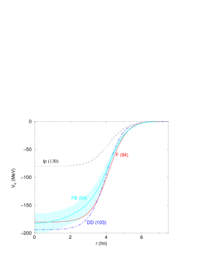
Figure 1: Real part of the $K^{-}$-Ni optical potential for various models and the values of $\chi^{2}$ for 65 data points in parentheses, see text.

Estimating the uncertainties of hadron-nucleus potentials as function of position is not a simple task. For example, in the ‘$t\rho$’ approach the shape of the potential is determined by the nuclear density distribution and the uncertainty in the strength parameter, as obtained from $\chi^{2}$ fits to the data, implies a fixed relative uncertainty at all radii, which is, of course, baseless. Details vary when more elaborate forms such as ‘DD’ or ‘F’ are used, but one is left essentially with analytical continuation into the nuclear interior of potentials that might be well-determined only close to the nuclear surface. ‘Model-independent’ methods have been used in analyses of elastic scattering data for various particles BFG89 to alleviate this problem. However, applying e.g. the Fourier-Bessel (FB) method in global analyses of kaonic atom data end up in too few terms in the series, thus making the uncertainties unrealistic in their dependence on position. This is illustrated in Fig. 1 by the ‘FB’ curve, obtained by adding a Fourier-Bessel series to a ‘$t\rho$’ potential. Only three terms in the series are needed to achieve a $\chi^{2}$ of 84 and the potential becomes deep, in agreement with the other two ‘deep’ solutions. The error band obtained from the FB method BFG89 is, nevertheless, unrealistic because only three FB terms are used. However, an increase in the number of terms is found to be unjustified numerically in this case.

In the present work we adopt a functional-derivative approach in order to get more realistic position-dependence of the uncertainties of $K^{-}$-nucleus potentials. The method is applied to the two types of potentials (‘shallow’ and ‘deep’) mentioned above and it is shown that deep potentials within nuclei are reliably obtained from fits to experimental results for kaonic atoms.

II Method

The radial sensitivity of exotic atom data was addressed before BFG97 with the help of a ‘notch test’, introducing a local perturbation into the potential and studying the changes in the fit to the data as function of position of the perturbation. The results gave at least a semi-quantitative information on what are the radial regions which are being probed by the various types of exotic atoms. In fact, the difference in that respect between deep and shallow kaonic atom potentials could be observed. However, the extent of the perturbation was somewhat arbitrary and in the present work we report on extending that approach to a mathematically well-defined limit.

In order to study the radial sensitivity of global fits to kaonic atom data, it is instructive to define the radial position parameter in a ‘natural’ way using, e.g., the known charge distribution for each nuclear species in the data base. The radial position $r$ is then defined as $r=R_{c}+\eta a_{c}$, where $R_{c}$ and $a_{c}$ are the radius and diffuseness parameters, respectively, of a two-parameter Fermi (2pF) charge distribution FBH95 . In that way $\eta$ becomes the relevant radial parameter when handling together data for several nuclear species along the periodic table. The value of $\chi^{2}$ can be regarded now as a functional of a global optical potential $V(\eta)$, i.e. $\chi^{2}=\chi^{2}[V(\eta)]$. The parameter $\eta$ is a continuous variable, however it is instructive to start the discussion of variations by assuming that the global optical potential is defined on a discrete set of grid points $\{\eta_{i},i=1\ldots N\}$, so that $\chi^{2}$ depends on a set of $N$ parameters $V_{i}=V(\eta_{i})$. The variation of $\chi^{2}$ due to a small change in these parameters is simply

$$d\chi^{2}=\sum_{i=1}^{N}\frac{\partial\chi^{2}}{\partial V_{i}}dV_{i}\;.$$ (1)

The equivalent expression for the continuous function $V(\eta)$ can be obtained by taking the limit for a very dense grid, leading to FD_wikipedia

$$d\chi^{2}=\int d\eta\frac{\delta\chi^{2}}{\delta V(\eta)}\delta V(\eta)\;,$$ (2)

where

$$\frac{\delta\chi^{2}[V(\eta)]}{\delta V(\eta^{\prime})}=\lim_{\sigma\rightarrow 0}\lim_{\epsilon\rightarrow 0}\frac{\chi^{2}[V(\eta)+\epsilon\delta_{\sigma}(\eta-\eta^{\prime})]-\chi^{2}[V(\eta)]}{\epsilon}\;$$ (3)

is the functional derivatives (FD) of $\chi^{2}[V]$. The notation $\delta_{\sigma}(\eta-\eta^{\prime})$ stands for an approximated $\delta$-function. From Eq. (2) it is seen that the FD determines the effect of a local change in the optical potential on $\chi^{2}$. Conversely it can be said that the optical potential sensitivity to the experimental data is determined by the magnitude of the FD. In practice the calculation of the FD was carried out by multiplying the best fit potential by a factor

$$f=1+\epsilon\delta_{\sigma}(\eta-\eta^{\prime})$$ (4)

using a normalized Gaussian with a range parameter $\sigma$ for the smeared $\delta$-function,

$$\delta_{\sigma}(\eta-\eta^{\prime})=\frac{1}{\sqrt{2\pi}\sigma}e^{-(\eta-\eta^{\prime})^{2}/2\sigma^{2}}.$$ (5)

For finite values of $\epsilon$ and $\sigma$ the FD can be approximated by

$$\frac{\delta\chi^{2}[V(\eta)]}{\delta V(\eta^{\prime})}\approx\frac{1}{V(\eta^{\prime})}\frac{\chi^{2}[V(\eta)(1+\epsilon\delta_{\sigma}(\eta-\eta^{\prime}))]-\chi^{2}[V(\eta)]}{\epsilon}\;.$$ (6)

The parameter $\epsilon$ was used for a fractional change in the potential and the limit $\epsilon\to 0$ was obtained numerically for several values of $\sigma$ and then extrapolated to $\sigma=0$. Good numerical stability and good convergence were obtained in all cases. Here $\eta$ and $\sigma$ are dimensionless variables.

III RESULTS AND CONCLUSIONS

The $K^{-}$-nucleus potentials used in the present work are taken from recent global fits MFG06 to kaonic atom data from ⁶Li to U, a total of 65 data points. A two-parameter fit with a $t\rho$ potential yields a total $\chi^{2}$ value of 130 whereas a four-parameter fit with $t(\rho)$ amplitudes yields $\chi^{2}$=84 for the 65 data points. In calculating FD for global fits radial positions were defined in terms of units of diffuseness relative to the charge radius, as described above. For several of the lightest nuclei harmonic oscillator densities are more appropriate and had indeed been used in the fits of Ref. MFG06 . These nuclei have been excluded from the calculations of FD for the global fits so as to have full consistency in the use of 2pF density distributions. That left 50 data points in the calculations of the FD.

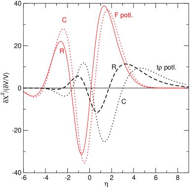
Figure 2: Functional derivatives of $\chi^{2}$ with respect to the full complex (C) and real (R) potential as function of $\eta$, where $r=R_{c}+\eta a_{c}$, with $R_{c}$ and $a_{c}$ the radius and diffuseness parameters, respectively, of the charge distribution. Results are shown for the $t\rho$ potential and for the $t(\rho)$ ‘F’ potential of Ref. MFG06 .

Figure 2 shows the FD for relative variations in the real potential and in the full complex potential. Inspecting the FD with respect to the imaginary potential (not shown) reveals additivity of the FD, hence the differences between the FD for the complex potential and for the real potential in the figure are the corresponding FD with respect to the imaginary potential. We note that the FD for the deep ‘F’ potential is dominated by the real part of the potential whereas for the ‘$t\rho$’ potential the two parts make similar contributions to the FD. The appearance of regions with negative FD need not be surprising because it means that some local variations in the shape of the potentials may cause further reduction in the values of $\chi^{2}$. Such variations are impossible in the $t\rho$ potential. However, such variations are included when the more flexible ‘F’ potential is introduced, and the minimisation process essentially follows implicitly the various FD. We avoid at present making a quantitative use of the local values of the FD, rather we identify with the help of the FD the radial regions to which the kaonic atom data are sensitive.

From Fig. 2 it can be inferred that the sensitive region for the real $t\rho$ potential is between $\eta=-1.5$ and $\eta=6$ whereas for the F potential it is between $\eta=-3.5$ and $\eta=4$. Recall that $\eta=-2.2$ correspond to 90% of the central charge density and $\eta=2.2$ correspond to 10% of that density. It therefore becomes clear that within the $t\rho$ potential there is no sensitivity to the interior of the nucleus whereas with the $t(\rho)$ ‘F’ potential, which yields greatly improved fit to the data, there is sensitivity to regions within the full nuclear density.

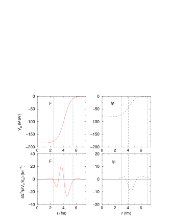
Figure 3: Real potentials (top) and FD (bottom) for the ‘F’ potential (left) and the $t\rho$ potential (right) for $K^{-}$ interaction with Ni. The regions between the vertical dotted lines indicate where the potentials are determined reliably, see text.

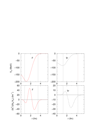
Figure 4: Same as fig. 3 but for ¹²C.

Figure 3 shows similar results for Ni, this time the radial variable is $r$, the radial position. Here $\sigma$ is in units of fm and therefore the FD is in units of fm^-1. On the left are shown the real potential (top) and the FD (bottom) for the real ‘F’ potential and on the right are shown the corresponding quantities for the $t\rho$ potential. The regions between the two vertical dotted lines indicate where variation of the potential will affect the fit to the data, thus suggesting the regions where the potentials are determined by experiment. The vertical dashed line indicates 50% of the central charge density. It is evident that for the ‘F’ potential the sensitivity extends to depths of 180 MeV at radii where the density is essentially the full nuclear density. Very similar results are obtained also for heavier nuclei, where, e.g. for Pb the distinction between the $t\rho$ and the ‘F’ potential is even greater than for Ni, with respect to the sensitivity of the experiment to depths and densities.

Finally, in Fig. 4 are shown similar results for ¹²C, which is one of the targets studied experimentally ABB05 and theoretically MFG06 . Again it is seen that with the ‘F’ potential the sensitive region is at smaller radii and higher densities compared to that for the $t\rho$ potentials.

In summary, it is found that the ‘deep’ $\bar{K}$-nucleus potentials, which yield excellent fits to all the kaonic atom data, are determined reliably to depths of 150-180 MeV at regions of almost the full nuclear matter density and consequently they may be reliably extrapolated to the nuclear interior. In contrast the ‘shallow’ type of potentials, which yield inferior fits to the data, are well determined only at the nuclear surface and one cannot infer from these what is the depth of the $\bar{K}$-nucleus potential in the nuclear interior. The different sensitivities result from the potentials themselves: the additional attraction provided by the deep potentials enhances the atomic wavefunctions within the nucleus BFG97 thus creating the sensitivity at smaller radii. We conclude that optical potentials derived from the observed strong-interaction effects in kaonic atoms are sufficiently deep to support strongly-bound antikaon states, but it does not necessarily imply that such states do exist. Moreover, the discrepancy between the very shallow chiral-motivated potentials ROs00 ; CFG01 and the deep phenomenological potentials remains an open problem.

References

- (1) M. Krell, Phys. Rev. Lett. 26, 584 (1971).
- (2) J.H. Koch et al., Phys. Rev. Lett. 26, 1465 (1971); Phys. Rev. C 5, 381 (1972).
- (3) see C.J. Batty, E. Friedman and A. Gal, Phys. Rep. 287, 385 (1997) and references therein.
- (4) A. Ramos and E. Oset, Nucl. Phys. A671, 481 (2000).
- (5) A. Cieplý et al., Nucl. Phys. A696, 173 (2001).
- (6) J. Mareš, E. Friedman and A. Gal, Nucl. Phys. A770, 84 (2006).
- (7) T. Suzuki et al., Phys. Lett. B597, 263 (2004).
- (8) T. Suzuki et al., Nucl. Phys. A754, 375c (2005).
- (9) T. Kishimoto et al., Nucl. Phys.A 754, 383c (2005).
- (10) M. Agnello et al., Phys. Rev. Lett. 94, 212303 (2005).
- (11) V.K. Magas et al., Phys. Rev. C 74, 025206 (2006).
- (12) N.V. Shevchenko, A. Gal and J. Mareš, Nucl-th/0610022.
- (13) see, for example, C.J. Batty et al., Adv. Nucl. Phys. 19, 1 (1989).
- (14) G. Fricke et al., At. Data Nucl. Data Tables 60, 177 (1995).
- (15) A simple and convenient introduction to the concept of functional derivative can be found in the wikipedia web site: http://en.wikipedia.org/wiki/Functional_derivative.