Effects of fluctuations on the initial eccentricity from the Color Glass Condensate in heavy ion collisions

Abstract

We introduce a modified form of the Kharzeev-Levin-Nardi (KLN) approach for nuclear collisions. The new ansatz for the unintegrated gluon distribution function preserves factorization, and the saturation scale is bound from below by that for a single nucleon. It also reproduces the correct scaling with the number of collisions at high transverse momentum. The corresponding Monte Carlo implementation allows us to account for fluctuations of the hard sources (nucleons) in the transverse plane. We compute various definitions of the eccentricity within the new approach, which are relevant for the interpretation of the elliptic flow. Our approach predicts breaking of the scaling of the eccentricity with the Glauber eccentricity at the level of about 30%.

I Introduction

The elliptic flow $v_{2}$ is one of the most important observables in high energy non-central nucleus-nucleus collisions at RHIC RHICexperiments . It is very sensitive to both the initial condition in the overlap zone, and to the subsequent evolution of the hot matter created in these collisions Ollitrault:1992bk . Predictions from ideal hydrodynamics with an initial condition from a Glauber type model and with a short thermalization time $\tau\leq 1$ fm/c are compatible with the elliptic flow data at low transverse momentum at RHIC hydroreview energies. This is one of the strongest indications of early thermalization and nearly perfect-fluid evolution of the quark-gluon plasma at RHIC.

It was found in Ref. Hirano:2005xf that ideal hydrodynamics with the initial condition taken from the Color Glass Condensate (CGC) approach HiranoNara04 overestimates the measured elliptic flow at RHIC. Since hadronic dissipative effects were taken into account by a hadronic transport model jam , additional dissipation in the quark-gluon phase would be required. The reason for the strong flow is that the KLN approach KLN01 predicts a larger eccentricity of the initial gluon distribution in the transverse plane than the Glauber model Hirano:2005xf ; Drescher:2006pi . A recent calculation within the classical Yang-Mills (CYM) approach on the lattice LV06 gave somewhat smaller values than predicted by the KLN model. Nevertheless, the eccentricity of the “overlap” region in coordinate space obtained from CYM still exceeds that predicted by the Glauber “wounded nucleon” model for soft processes.

The eccentricity $\varepsilon$ is defined in the transverse plane $\bm{r}_{\perp}=(r_{x},r_{y})$ perpendicular to the beam axis by

$$\varepsilon=\frac{\langle r_{y}^{\,2}{-}r_{x}^{\,2}\rangle}{\langle r_{y}^{\,2}{+}r_{x}^{\,2}\rangle}~{}.$$ (1)

The average may be taken with respect to either energy or particle density (or entropy, if rapid thermalization is assumed). In the ideal hydrodynamical limit Bhalerao05 , elliptic flow only depends on the density and on $\varepsilon$. Therefore, it is very important to know the initial conditions to extract properties of hot and dense matter created in nucleus-nucleus collisions.

This paper is a continuation of Ref. Drescher:2006pi , where we computed the eccentricity in the initial stage of heavy ion collisions within the KLN approach, and showed that the large eccentricity predicted by the $k_{\perp}$-factorization approach is generic, as it does not depend on the details of the unintegrated gluon distribution function (uGDF) such as the presence of leading-twist shadowing and an extended geometric scaling window DHJ ; KKT03 ; Braun:2000bh .

The predictions of the CGC framework are consistent with RHIC data for the centrality, energy and rapidity dependence of the multiplicity of charged hadrons if the square of the saturation scale (averaged over the transverse plane) is defined to be proportional to the number of participants KLN01 ; Drescher:2006pi ; Baier:2002bt ; Armesto:2004ud . In this paper, we shall consider in more detail the relation between the different definitions of the saturation scales (see also the short note in Ref. Drescher:2006pi ).

The eccentricity could of course fluctuate for many reasons, and it was recently argued that event-by-event flow fluctuations can affect the elliptic flow obtained via correlation methods  Miller:2003kd ; Manly:2005zy ; Voloshin:2006gz ; Bhalerao:2006tp . In order to explore such fluctuation effects in the CGC picture, we employ a Monte-Carlo implementation of the KLN approach which accounts for fluctuations of the high-rapidity “hard sources” (nucleons) in the transverse plane. This leads naturally to a factorized version of the KLN approach, where the uGDFs depend only on the properties of a single nucleus. We analyze the effects of the fluctuations on the eccentricity by using different definitions of the eccentricities  Miller:2003kd ; Manly:2005zy ; Voloshin:2006gz ; Bhalerao:2006tp . This is relevant to the study of the effects of fluctuations on $v_{2}$  Aguiar:2001ac ; Hama ; Andrade:2006yh ; Zhu:2005qa .

II Gluon production in the KLN approach

In the $k_{\perp}$-factorization approach GLR83 , the number distribution of produced gluons is given by

$$\frac{dN_{g}}{d^{2}r_{\perp}dy} = \frac{4N_{c}}{N_{c}^{2}-1}\int^{p_{\perp}^{\mathrm{max}}}\frac{d^{2}p_{\perp}}{p^{2}_{\perp}}\int^{p_{\perp}}\frac{d^{2}k_{\perp}}{4}\;\alpha_{s}$$

$$\times \phi_{A}(x_{1},(\bm{p}_{\perp}+\bm{k}_{\perp})^{2}/4)\;\phi_{B}(x_{2},(\bm{p}_{\perp}{-}\bm{k}_{\perp})^{2}/4)$$

with $N_{c}=3$ the number of colors. Here, $p_{\perp}$ and $y$ denote the transverse momentum and the rapidity of the produced gluons, respectively. The light-cone momentum fractions of the colliding gluon ladders are then given by $x_{1,2}=p_{\perp}\exp(\pm y)/\sqrt{s}$, where $\sqrt{s}$ denotes the center of mass energy and $y$ is the rapidity of the produced gluon. We set $p_{\perp}^{\mathrm{max}}$ such that the minimal saturation scale $Q_{s,\min}(x_{1,2})$ in the above integration is $\Lambda_{QCD}=0.2$ GeV (see, however, below). The KLN approach KLN01 employs the following uGDF:

$$\phi(x,k_{\perp}^{2};\bm{r}_{\perp})\sim\frac{1}{\alpha_{s}(Q^{2}_{s})}\frac{Q_{s}^{2}}{{\rm max}(Q_{s}^{2},k_{\perp}^{2})}~{},$$ (3)

where $Q_{s}$ denotes the saturation momentum at the given momentum fraction $x$ and transverse position $\bm{r}_{\perp}$. The overall normalization is determined by the multiplicity at midrapidity for the most central collisions.

In Refs. KLN01 ; HiranoNara04 ; Hirano:2005xf ; Drescher:2006pi , the saturation scale for nucleus $A$ is taken to be proportional to the density of participants, $n^{A}_{\mathrm{part}}(\bm{r}_{\perp})$, which in turn is obtained from the thickness functions $T_{A}$ and $T_{B}$:

$$n^{A}_{\mathrm{part}}(\bm{r}_{\perp}) = T_{A}(\bm{r}_{\perp}+\bm{b}/2)$$ (4)

$$\times (1-(1-\sigma_{NN}T_{B}(\bm{r}_{\perp}-\bm{b}/2)/B)^{B})~{}.$$

$\bm{b}=(b,0)$ is the impact parameter vector in the transverse plane and $\sigma_{NN}$ is the nucleon-nucleon inelastic cross section.

The density of participants is not a universal quantity which depends only on the properties of a single nucleus. In the following we propose a modified form of the KLN approach where factorization is manifest and show that the $Q_{s}^{2}\sim n_{\mathrm{part}}$ definition is in fact a good approximation for computing the multiplicity of gluons. Other quantities such as the energy density, however, do behave somewhat differently.

III Factorized KLN formula for nucleus-nucleus collisions

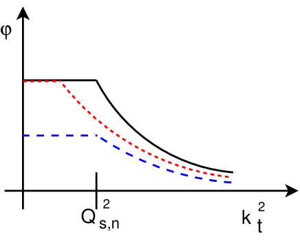
Figure 1: (Color online) Schematic sketch of different constructions of the uGDF. The full line corresponds to the uGDF of a single nucleon, the other lines to that of a nucleus at its surface. The dotted line corresponds to the the definition from Eq.(6) while the dashed line is for Eq. (5).

Generically, it is reasonable to define the squared saturation scale to be proportional to the density of nucleons. However, a problem arises near the edge of a nucleus where the density is small. There, the thickness function $T_{A}$ is small: only for some configurations of nucleons do we actually find a nucleon at that position. Let us denote this probability of finding at least one nucleon at a given transverse coordinate as $p_{A}$. For configurations where indeed there is one single nucleon at the given ${\bf r}_{\perp}$, the uGDF should be that of a nucleon: $\phi=\phi(Q_{s,n}^{2})$. However, the average $\phi_{A}({\bf r}_{\perp})$ would then be

$$\phi_{A}=p_{A}\phi(Q^{2}_{s,n})$$ (5)

rather than

$$\phi_{A}=\phi(Q^{2}_{s,n}p_{A})~{}.$$ (6)

This is illustrated in Fig. 1. The essential point is that one has to average the uGDF itself, and not its argument $T_{A}$. Expressing the uGDF in terms of $T_{A}$, the relevant variable would be $T_{1A}$, which is the density of nucleus $A$ averaged only over those configurations with at least one nucleon at a given transverse position. This quantity can be obtained by averaging over the thickness functions of $i\geq 1$ nucleons,

$$T_{1A}\equiv\langle t_{A}\rangle_{i\geq 1}=\frac{\sum_{i=1}p_{A}(i)~{}t_{A}(i)}{\sum_{i=1}p_{A}(i)}=\frac{T_{A}}{p_{A}},$$ (7)

where $t_{A}(i)$ is the thickness function for $i$ nucleons in a row. This allows us to construct an uGDF in the following way,

$$\phi_{A}=p_{A}~{}\phi\left(\frac{T_{A}}{p_{A}}\right)~{}.$$ (8)

Here, and in the following, we use a short-hand notation for the dependence of $\phi$ on some density $\rho$: $\phi(\rho)\equiv\phi(Q_{s}^{2}(\rho))$. The uGDF (8) respects factorization, since it depends only on the properties of a single nucleus. The saturation scale is then parameterized as

$$Q^{2}_{s,A}(x,\bm{r}_{\perp})=2\,{\rm GeV}^{2}\left(\frac{T_{A}(\bm{r}_{\perp})/p_{A}(\bm{r}_{\perp})}{1.53}\right)\left(\frac{0.01}{x}\right)^{\lambda},$$ (9)

$p_{A}$ can be taken from the Glauber definition of $n_{\mathrm{part}}$:

$$p_{A}=(1-(1-ST_{A}/A)^{A}).$$ (10)

In this case, $S$ is a sampling area and not the nucleon-nucleon inelastic cross section as in the Glauber model. Nevertheless, these quantities are related to each other, since $S$ should be on the order of the area of the nucleon. One could fix its value in such a way that one recovers the saturation scale of a nucleon in the limit $T_{A}\rightarrow 0$, since

$$\lim_{T_{A}\rightarrow 0}\frac{T_{A}}{p_{A}}=\frac{1}{S}.$$ (11)

For our simulations we will however use the value of the inelastic cross section at RHIC energy, since then the results are more directly comparable to the original KLN ansatz. The saturation scale of a nucleon is then equal to $Q_{s,n}^{2}=2.0~{}\mathrm{GeV}^{2}/(4.2\times 1.53)=0.31~{}\mathrm{GeV}^{2}$. We refer to this approach as the factorized KLN (fKLN) model.

Next, we explore the relation to the original KLN ansatz, where the saturation momentum is defined via $n_{\mathrm{part}}$. The transverse density of produced gluons can roughly be expressed analytically in terms of the saturation scales as KLN01

$$\frac{dN_{g}}{dyd^{2}\bm{r}_{\perp}}\sim Q^{2}_{s_{,}\min}\left(2+\log\left(\frac{Q^{2}_{s,\max}}{Q^{2}_{s,\min}}\right)\right),$$ (12)

where, $Q_{s,\max}$ and $Q_{s,\min}$ denote the larger and the smaller value of the two saturation scales in opposite nuclei at any fixed position in the transverse plane. It is easy to see that this function is homogeneous of order one in both $Q_{s,A}^{2}$ and $Q_{s,B}^{2}$, or in the corresponding densities which appear in the definition of the saturation scales. The $k_{\perp}$-factorization formula with the new definition of the uGDF (fKLN approach) now takes the form:

$$\frac{dN_{g}}{dyd^{2}\bm{r}_{\perp}}\sim\int\frac{d^{2}p_{\perp}}{p_{\perp}^{2}}\int d^{2}k_{\perp}p_{A}p_{B}\phi(T_{A}/p_{A})\phi(T_{B}/p_{B}).$$ (13)

Due to the homogeneity, we can move the prefactors in eq. (13) into the arguments of the uGDF. If $S$ is the nucleon-nucleon inelastic cross section $\sigma_{NN}$, we have $n_{\mathrm{part},A}=T_{A}p_{B}$. This leads to the original KLN definition of the uGDF, where the saturation scales depend on the participant densities:

$$\frac{dN_{g}}{dyd^{2}\bm{r}_{\perp}} \sim \int\frac{d^{2}p_{\perp}}{p_{\perp}^{2}}\int d^{2}k_{\perp}\phi(p_{A}p_{B}T_{A}/p_{A})\phi(p_{A}p_{B}T_{B}/p_{B})$$ (14)

$$= \int\frac{d^{2}p_{\perp}}{p_{\perp}^{2}}\int d^{2}k_{\perp}\phi(n_{\mathrm{part},A})\phi(n_{\mathrm{part},B})~{}.$$

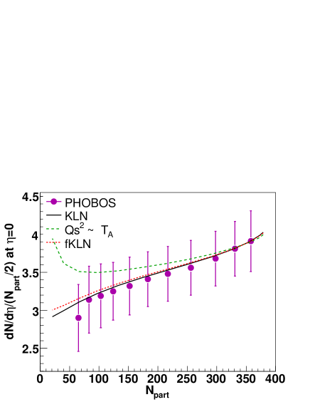
Figure 2: (Color online) Centrality dependence of the multiplicity for the different assumptions of the uGDF. Eq. (6) gives a significant overestimate of the multiplicity in the peripheral collisions. The original KLN ansatz, where $Q^{2}_{s}\sim n_{\mathrm{part}}$ is very similar to the fKLN result which uses Eq. (13). Data from PHOBOS phobos .

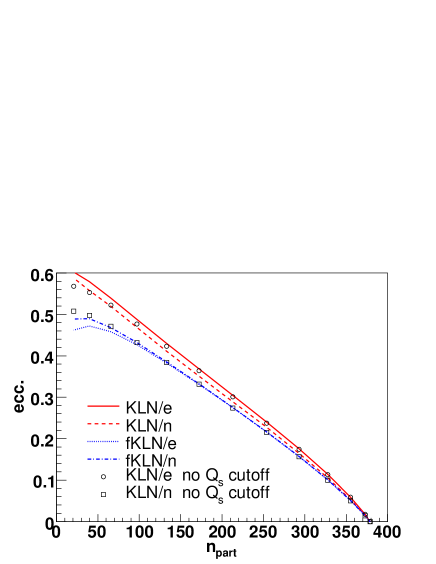
Figure 3: (Color online) The initial eccentricity $\varepsilon$ at midrapidity as a function of the number of participants for 200 $A$ GeV Au+Au collisions: KLN/e (KLN/n) corresponds to the KLN result using the energy (number) density as the weight in the definition of the eccentricity. fKLN results follow the same notation. The KLN results without a saturation scale cutoff are shown by symbols.

The expression (13) involving the new definition of the uGDF can now be integrated numerically. The centrality dependence of the multiplicity at midrapidity is shown in Fig. 2, assuming that the hadron yield is proportional to the yield of produced gluons. For comparison, we also show the result corresponding to the definition $Q^{2}_{s}\sim T_{A}$ in the $k_{\perp}$-factorization formula, which clearly overshoots the data for peripheral collisions. On the other hand, the fKLN approach is rather similar to the original KLN approach. This is due to the fact that the single-inclusive gluon cross section is homogeneous of order one in both arguments, as discussed above.

In Fig. 3, we compare the eccentricities obtained from fKLN (eq. (1)) and KLN. We plot two cases, where we use the transverse energy density $dE_{\perp}/dyd^{2}{\bf r}_{\perp}$ and the number density as a weight in the definition of the eccentricity. The eccentricity from fKLN is somewhat lower than the one from KLN, especially for more peripheral collisions. This is due to the fact that the transverse energy distribution from the KLN approach is homogeneous of order 3/2, because of another factor of $Q_{s,\max}$ DMcL :

$$\frac{dE_{\perp}}{d^{2}{\bf r}_{\perp}dy}\sim Q_{s,min}^{2}Q_{s,max}\;\log\frac{Q_{s,max}^{2}}{Q_{s,min}^{2}}.$$ (15)

As a consequence, the energy density distributions in the transverse plane from KLN and fKLN, respectively, are somewhat different.

If one uses the number density of produced gluons rather than their energy density as a weight in the definition of the eccentricity, one would expect that the fKLN form reproduces the KLN result, since the same arguments hold as for the multiplicity. However, we have found that the fKLN prediction for the eccentricity with the number density as a weight is almost identical to the above result (which employed energy density as a weight). This can be traced back to the above-mentioned cut-off $Q_{s,min}=\Lambda_{\rm QCD}$. In the fKLN model no such cutoff is needed as the minimal saturation momentum never drops below the saturation momentum of a single nucleon, by construction. Rather, the probabilities $p_{A}$, $p_{B}$ of encountering at least one nucleon vanish at the surface of the overlap region. Even though it does not make much sense physically, technically we can set the minimal saturation scale in the KLN model to zero. Then the eccentricity from the KLN approach agrees well with the one from the factorized fKLN form as seen in Fig. 3.

IV Monte-Carlo implementation of the KLN approach

According to the ideas of McLerran and Venugopalan, the gluon field of a sufficiently large nucleus can be viewed as a classical Yang-Mills field MV . Particle production in high-energy hadronic collisions can then be calculated by solving the Yang-Mills equations in the forward light-cone with a boundary condition corresponding to classical sources on its two branches. Real time solutions of the classical Yang-Mills fields on the lattice were obtained, for example, in Refs. KV ; Krasnitz:2002mn ; Lappi . Those numerical solutions are usually averaged over many different initial conditions (configurations of the color-charge sources).

Here, we calculate the thickness function used for determining the saturation scale with a Monte Carlo method. There are two advantages of doing this. First, the Monte-Carlo implementation naturally leads to a definition of the saturation momentum in terms of the thickness functions (which preserves factorization). Second, we can study the effects of event-by-event fluctuations on the eccentricity within the KLN approach. We only consider fluctuations of the positions of the nucleons, which were previously studied in Refs. Miller:2003kd ; Manly:2005zy ; Voloshin:2006gz ; Bhalerao:2006tp within the Glauber approach. We note that in Ref. Krasnitz:2002mn , a similar method was employed to impose a color neutrality condition for a each nucleon in the classical McLerran-Venugopalan model in order to simulate collisions of finite nuclei.

IV.1 Model

Let us now construct a Monte Carlo model for gluon production for each configuration of nucleons within the colliding nuclei (denoted as MC-KLN). We first determine the positions of $A$ nucleons according to the Woods-Saxon distribution. Correlations among the nucleons are neglected at present but could in principle be taken into account. They tend to reduce fluctuations somewhat Baym:1995cz .

The local density of nucleons, $t_{A}$, is then obtained by counting nucleons within a tube of radius $r_{\mathrm{max}}=\sqrt{S/\pi}$ around a given transverse coordinate ${\bf r}_{\perp}$:

$$t_{A}(\bm{r}_{\perp})=\frac{\mathrm{number~{}of~{}nucleons}}{S}$$ (16)

The area $S$ is the sampling area over which we count nucleons. The average $\left<t_{A}(\bm{r}_{\perp})\right>$ reproduces the convoluted thickness function $\widetilde{T}_{A}(\bm{r}_{\perp})$ with a sampling profile $f({\bm{r}}_{\perp})=\frac{1}{S}\Theta(r_{max}-|{\bm{r}}_{\perp}|)$:

$$\left<t_{A}({\bm{r}}_{\perp})\right>=\widetilde{T}_{A}({\bm{r}}_{\perp})=\int d^{2}{\bm{r}}^{\prime}_{\perp}~{}T_{A}({\bm{r}}^{\prime}_{\perp})~{}f(\bm{r}_{\perp}-{\bm{r}}^{\prime}_{\perp})$$ (17)

In the limit $S\rightarrow 0$, $\widetilde{T}_{A}$ equals $T_{A}$. This limit can be taken in a Monte Carlo by the oversampling (“test-particle”) technique, whereby the sampling area $S$ is reduced by some factor $n$ and the number of nucleons is increased by the same factor; each nucleon then carries a weight $1/n$. (We found that oversampling by a factor of $n=100$ gives stable results.) It is not appropriate to simply decrease $S$. While this would reproduce the mean value of $T_{A}$, it would also change the fluctuations in the number of nucleons at a given position, since each nucleon would contribute $n/S$ to the density. With the oversampling technique each nucleon has a weight $1/n$ and therefore contributes $1/S$ to the density, which is independent of $n$. However, correlations between neighboring points in the transverse plane are destroyed. Therefore, event-by-event observables cannot be obtained with this method; we employed it only to test convergence of our MC implementation to the “mean-field” results presented above and for the computation of averaged observables. In the following simulations, we choose $S=\sigma_{\rm inel}$ as in the mean-field fKLN approach above.

We then follow the same procedure to compute $t_{B}(\bm{r}_{\perp})$, thereby generating two configurations for nucleus $A$ and $B$, respectively, at a specified impact parameter. The saturation scale at a given transverse coordinate is then given by

$$Q^{2}_{s,A}(x,\bm{r}_{\perp})=2\,{\rm GeV}^{2}\left(\frac{t_{A}({\bm{r}}_{\perp})}{1.53}\right)\left(\frac{0.01}{x}\right)^{\lambda}~{},$$ (18)

and similarly for nucleus $B$. It is clear that this choice of the saturation scale only depends on the properties of one nucleus, and therefore respects factorization.

For each generated configuration we apply the $k_{\perp}$-factorization formula (II) to obtain the distribution of produced gluons in the transverse plane. We then average over many collisions to compute observables and their fluctuations.

Finally, we establish the relation between MC-KLN and fKLN. The average uGDF which is effectively employed in the MC-KLN model may be written as

$$\phi_{A}=\sum_{i=0}^{A}p_{A}(i)\phi(t_{A}(i))=\sum_{i=1}^{A}p_{A}(i)\phi(t_{A}(i))~{},$$ (19)

where we used $t_{A}(0)=0$. The fKLN uGDF may be obtained from the approximation where $t_{A}(i)$ is replaced by the average, $t_{A}(i)\to T_{1A}$:

$$\phi_{A}\approx\sum_{i=1}^{A}p_{A}(i)\phi(T_{1A})=p_{A}\phi(T_{A}/p_{A}),$$ (20)

where $\sum_{i=1}p_{A}(i)=p_{A}$ was used.

IV.2 Results

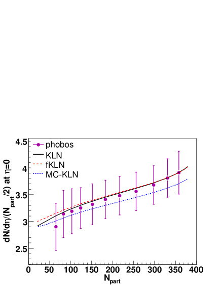
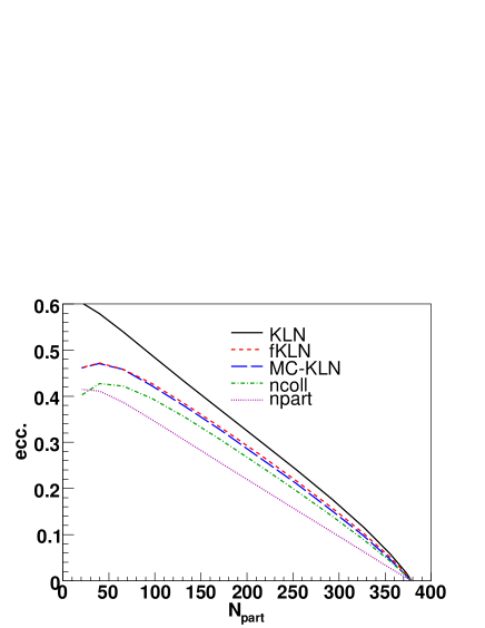
Figure 4: (Color online) Centrality dependence of the multiplicity in Au+Au collisions for $\sqrt{s_{NN}}=200$ GeV for the fKLN and MC-KLN models. All curves have the same normalization, we adjusted the result for KLN to the two most central bins. The data is from PHOBOS phobos .

Figure 5: (Color online) The eccentricity $\varepsilon$ in Au+Au collisions predicted by the various models. fKLN and MC-KLN give almost identical results. The MC-KLN result was obtained using the oversampling technique with $n=100$, which corresponds roughly to a delta function sampling profile, just as used in the fKLN model.

First, we show the centrality dependence of the multiplicity from the MC-KLN model in Fig. 5 together with the result of the original KLN approach. For clarity, we have not adjusted the overall normalization to the most central events. The multiplicity as a function of the centrality from MC-KLN is very similar to the original KLN and to the fKLN approach. The overall normalization is about 5% lower. The reason is that the multiplicity as a function of the density has negative curvature (second derivative), so fluctuations reduce the multiplicity.

In Fig. 5, we compare the eccentricity among the various approaches. Since the fKLN result was obtained using a delta function sampling profile (by using $T_{A}$ instead of $\widetilde{T}_{A}$), we employed the oversampling technique with a factor $n=100$ for the MC-KLN model. This way, the two models use the same sampling profile and the results are comparable. It can be seen that the eccentricity from MC-KLN is almost identical to the fKLN scaling, which is slightly higher than $n_{\rm coll}$ scaling. Note that any additional fluctuation (e.g. in the evolution of the BFKL-ladders) would not influence the standard eccentricity (1), which is due to its definition; the denominator and the numerator are averaged separately and both are linear functions of the weight.

The eccentricity from the CYM approach LV06 behaves similar to the number of collision scaling in the Glauber model. Note that the CYM approach in Ref. LV06 does not include effects of nucleon fluctuations. Hence, we conclude that the main reason for the reduced eccentricity as compared to the original KLN approach is the use of the thickness functions in the definition of the saturation scale as argued in Ref. LV06 . Both, the CYM approach from Ref. LV06 and our fKLN approach, however, predicted larger $\varepsilon$ than the Glauber model for soft collisions where $dN/dyd^{2}{\bf r}_{\perp}$ scales with the density of participants $n_{\rm part}$.

IV.3 Eccentricity Fluctuations

We now turn to a comparison of various definitions of the eccentricity which are relevant for the scaling properties of the experimental data for $v_{2}$. Since we now consider event-by-event variables, we cannot use oversampling any more. This changes the results somehow, since the interaction range of the nucleon-nucleon interaction plays some role. In Appendix 10, we summarize how to include the interaction range in the numerical computations of the number of participants and collisions.

First we define the participant eccentricity $\varepsilon_{\mathrm{part}}$ according to Ref. Manly:2005zy in order to account for fluctuations in the directions of the major axes of the overlap region and of the “center of gravity”,

$$\varepsilon_{\mathrm{part}}=\frac{\sqrt{(\sigma^{2}_{y}-\sigma^{2}_{x})^{2}+4\sigma^{2}_{xy}}}{\sigma^{x}_{y}+\sigma^{2}_{x}},$$ (21)

where $\sigma_{x}$ and $\sigma_{y}$ are the RMS widths of the participant nucleon distribution projected on the $r_{x}$ and $r_{y}$ axes, respectively, and $\sigma_{xy}=\langle xy\rangle-\langle x\rangle\langle y\rangle$. We also compute

$$\varepsilon\{2\}\equiv\sqrt{\langle\varepsilon^{2}_{\mathrm{part}}\rangle}$$ (22)

which is closely related to the event-plane method of the measurements of elliptic flow. For four-particle cumulants of azimuthal correlations  Bhalerao:2006tp we have:

$$\varepsilon\{4\}\equiv\left(2\langle\varepsilon^{2}_{\mathrm{part}}\rangle^{2}-\langle\varepsilon^{4}_{\mathrm{part}}\rangle\right)^{1/4}.$$ (23)

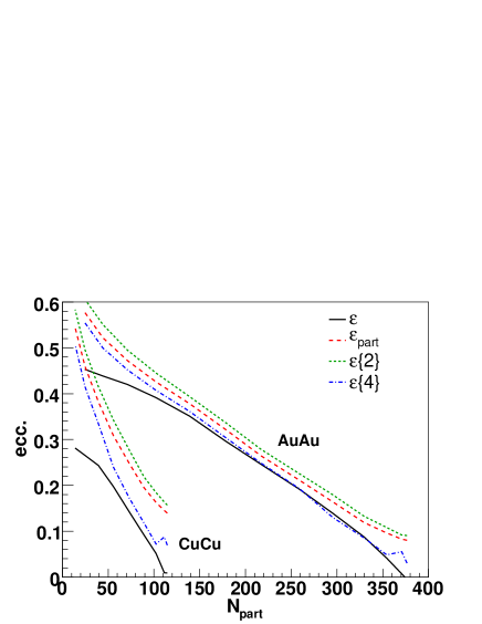
Figure 6: (Color online) Various eccentricities for the MC-KLN model. No oversampling was used, which corresponds to a finite range sampling profile.

In Fig. 6 we show $\varepsilon_{\mathrm{part}}$, $\varepsilon\{2\}$, $\varepsilon\{4\}$ together with the standard $\varepsilon$ from the MC-KLN model, for Au+Au and Cu+Cu collisions at $\sqrt{s}=200$  GeV, using again the energy density as weight in the eccentricities. Compared to Fig. 5, the standard eccentricity is reduced somewhat, since we did not use the oversampling technique in this plot (see also Fig. 10 of Appendix A). As observed before Manly:2005zy ; Voloshin:2006gz ; Ollitrault:1992bk in the Glauber model approach, $\varepsilon\{2\}$ deviates most from the standard definition, and the deviation is much larger for smaller systems. Since the source of fluctuations in this work is the position of the nucleons, the influence of the fluctuations on the results is very similar to that of the Glauber model approach.

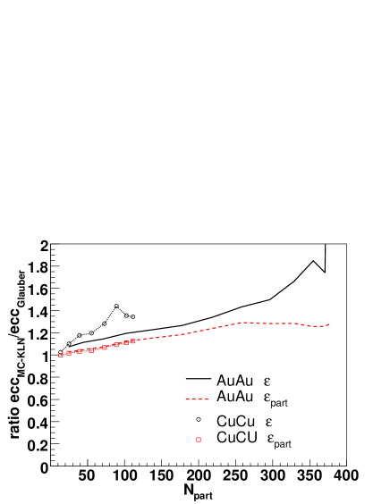
Figure 7: (Color online) The standard eccentricity $\varepsilon$ and $\varepsilon_{\mathrm{p}art}$ of MC-KLN relative to the Glauber model result.

A detailed comparison to the Glauber eccentricity can be seen in Fig. 7, where we show the ratio of the eccentricity obtained by the MC-KLN model to the eccentricity of the Glauber model. In Au+Au collisions, we see an increase of the ratio $\varepsilon_{\mathrm{MC-KLN}}/\varepsilon_{\mathrm{Glauber}}$ by more than 50% for central and 10% for peripheral collisions. Comparing to Cu+Cu collisions, we notice a discrepancy of the ratios for a system size above 50 participants. Using the $\varepsilon_{\mathrm{p}art}$ definition, which accounts for fluctuations of the major axes, we observe that both systems follow the same curve and the enhancement is not more than 30%. Therefore, precise experimental data would be able to distinguish MC-KLN from the usual Glauber scaling by examining the scaling properties of the elliptic flow.

So far we assumed that additional fluctuations (e.g. from the evolution of the BFKL-ladders) in the gluon production are negligible. While this is true for the standard definition of the eccentricity, it does not necessarily hold for event-by-event definitions such as $\varepsilon_{\mathrm{part}},\varepsilon\{2\}$ and $\varepsilon\{4\}$. In these cases, the eccentricity might increase. We tested this assumption by including simple Poissonian fluctuations in the gluon number but found that $\varepsilon\{2\}$ increased by only about $0.02$.

V Discussion and conclusions

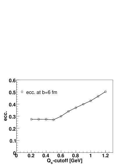
Figure 8: The eccentricity as a function of the $Q_{s,min}$ low-density cutoff.

We developed a simple model which includes fluctuations of the positions of the nucleons in the $k_{\perp}$-factorization formula. It naturally leads to a gluon production cross section which respects factorization. The multiplicity as a function of centrality does not change much as compared to the original KLN approach but the predicted eccentricity is somewhat lower.

It should be noted, however, that the gluon distribution calculated here corresponds to very early times on the order of $\sim 1/Q_{s}$. Therefore, it is not necessarily identifiable with the initial condition for hydrodynamics since it could be modified during the thermalization stage. A detailed analysis requires simulations of the time evolution from the early production time $1/Q_{s}$ until thermalization. This could be done within parton cascade models molnar01 ; Xu:2004mz which should be coupled to the Yang-Mills equations describing the soft gluons NaraCPIC . This is beyond the purpose of the present paper.

Our qualitative expectation is that the low-density surfaces of the overlap zone may not thermalize (and should therefore not be included in the initial condition for hydrodynamics), while the gluons produced closer to the center do. We can assess the consequences of such a simple picture by increasing the minimal saturation scale $Q_{s,min}(x_{i})$ which acts as a cutoff. This amounts to removing the very high-$p_{\perp}$ gluon jets as well as the low-density part of the bulk near the surface. The effect on the eccentricity is shown in Fig. 8. One observes that the eccentricity increases significantly with the cutoff. The fact that $\varepsilon$ is flat up to $Q_{s,min}=0.5$ GeV is due to the construction of the fKLN uGDF: the saturation scale never drops below that for a single nucleon and smaller cutoffs therefore do not matter. Since no thermalization is expected to occur in $p+p$ or $p+A$ collisions, the relevant cutoff for the hydrodynamic initial condition might be well above $\sim 0.5$ GeV. It would be interesting to study the hydrodynamical evolution of various initial conditions in order to check how sensitive the elliptic flow responds.

Another advantage of the fKLN uGDF is that it reproduces the correct scaling of the multiplicity with $n_{\rm ncoll}=\sigma T_{A}T_{B}$ at high $p_{t}$ in the DGLAP regime. This is not the case for the original KLN ansatz. There, the high-$p_{t}$ multiplicity also scales with $Q_{s,A}^{2}Q_{s,B}^{2}$, but with $Q_{s,2}\sim n_{\mathrm{part}}$, one does not recover scaling with $T_{A}T_{B}$. As we have shown, the naive modification to $Q_{s}^{2}\sim T_{A}$ does not help, since the saturation momentum at the edge of a nucleus drops below that for a single nucleon, and the $k_{\perp}$-factorization formula does not reproduce the centrality dependence of the multiplicity. Our fKLN (and MC-KLN) uGDF solves these problems simultaneously: while it fits correctly the measured centrality dependence of the multiplicity, it does not break factorization, the nuclear saturation scale is bound from below by the saturation scale of a single nucleon, and it reproduces the correct $n_{\rm coll}$ scaling at high $p_{t}$.

Appendix A Number of participants and Interaction profiles

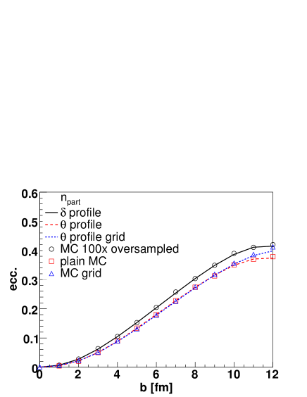
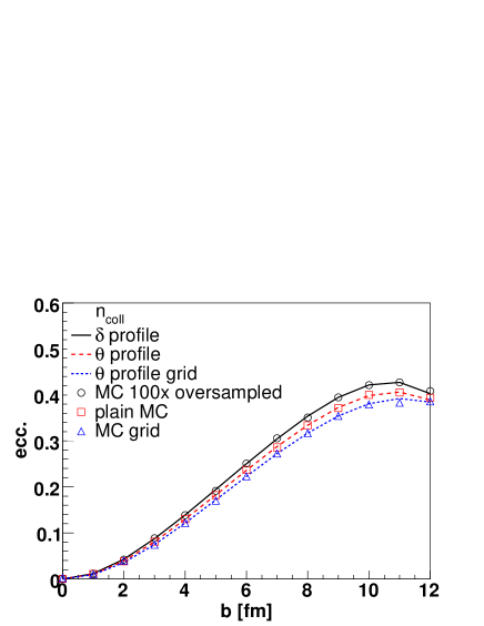
Figure 9: (Color online) Eccentricity for the Glauber model with number of participants scaling of $dN/d^{2}{\bf r}_{\perp}$ obtained with the following methods: delta function interaction profile (point nucleons), step function (hard sphere nucleons) and step function with sampling on a grid.

Figure 10: (Color online) Same as Fig. 10 for number of collisions scaling.

A.1 Delta function interaction profile

The densities of participants in the transverse plane are given by

$$n_{{\rm part},A} = T_{A}\left(1-\left(1-\sigma{T}_{B}/B\right)^{B}\right)$$ (24)

$$n_{{\rm part},B} = T_{B}\left(1-\left(1-\sigma{T}_{A}/A\right)^{A}\right)$$ (25)

$$n_{\rm coll} = \sigma T_{A}{T}_{B}~{}.$$ (26)

These definitions assume a delta function interaction profile $f(r)=\sigma\delta(r)$. In a Monte Carlo model, one can approximate the delta function via the oversampling technique: $\sigma\rightarrow\sigma/n$ and $A\rightarrow An$, attributing a weight $1/n$ to each nucleon.

A.2 Finite range interaction profile

Next, we discuss how to calculate the number of participants and the number of collisions respecting finite range interaction. The thickness function is convoluted with the interaction profile,

$$\widetilde{T}_{A}({\bm{r}}_{\perp}) = \int d^{2}{\bm{r}}^{\prime}_{\perp}\frac{f({\bm{r}}_{\perp}-{\bm{r}}^{\prime}_{\perp})}{\sigma}T_{A}({\bm{r}}^{\prime}_{\perp})~{}.$$

Therefore, we have

$$n_{{\rm part},A} = T_{A}\left(1-(1-\sigma\widetilde{T}_{B}/B)^{B}\right)$$ (27)

$$n_{{\rm part},B} = T_{B}\left(1-(1-\sigma\widetilde{T}_{A}/A)^{A}\right)~{}.$$ (28)

The number of collisions can be derived in a similar way. Special attention is needed when specifying the location of the collision: $n_{\rm coll}=\sigma T_{A}\widetilde{T}_{B}$ locates the collision at the participating nucleon from nucleus A and $n_{\rm coll}=\sigma T_{B}\widetilde{T}_{A}$ locates the collision at the nucleon from nucleus $B$. The following definition

$$n_{\rm coll}=\frac{\sigma}{2}(T_{A}\widetilde{T}_{B}+\widetilde{T}_{A}T_{B})$$ (29)

uses the center-of-mass position and is symmetric under the exchange $A\leftrightarrow B$.

The definitions (27-29) agree with a straightforward Glauber Monte Carlo, where the positions of the nucleons are sampled according to the Woods-Saxon distribution, and where the profile functions determine whether an inelastic interaction for a given pair of nucleons occurs.

A.3 Monte Carlo Method on a grid

Sampling the number of participants within the interaction range corresponds to using the convoluted thickness functions for both nuclei. The corresponding definitions for the participant and collision densities are:

$$n_{{\rm part},A} = \widetilde{T}_{A}\left(1-(1-\sigma\widetilde{T}_{B}/B)^{B}\right)$$ (30)

$$n_{{\rm part},B} = \widetilde{T}_{B}\left(1-(1-\sigma\widetilde{T}_{A}/A)^{A}\right)$$ (31)

$$n_{\rm coll} = {\sigma}\widetilde{T}_{A}\widetilde{T}_{B}$$ (32)

Here the cross section is used in two ways: once for determining the interaction, and once for sampling the nucleons over the transverse area given by the cross section. Strictly speaking, this implies double-counting but this method provides good approximations to eqs.(27-29), as shown below.

Figs. 10 and 10 show the eccentricity for number of participants and number of collisions scaling obtained with different interaction profiles and sampling methods. The normal definition of $T_{A}$ corresponds to a delta function interaction profile. It is reproduced by a Monte Carlo oversampling technique. A different interaction profile (in this case, a $\theta$-function: $f(r)=\theta(\sqrt{\sigma/\pi}-r)$) leads to formulas (27-29). The corresponding Monte Carlo method (denoted as plain MC) is straightforward: the profile function determines the probability for an interaction for each nucleon-pair. The third method, Monte Carlo on a grid, samples the nucleon densities within the interaction range. It is very similar to plain Monte Carlo. However, the number of collision scaling is somewhat smaller.