Interaction of Regular and Chaotic States

Abstract

Modelling the chaotic states in terms of the Gaussian Orthogonal Ensemble of random matrices (GOE), we investigate the interaction of the GOE with regular bound states. The eigenvalues of the latter may or may not be embedded in the GOE spectrum. We derive a generalized form of the Pastur equation for the average Green’s function. We use that equation to study the average and the variance of the shift of the regular states, their spreading width, and the deformation of the GOE spectrum non–perturbatively. We compare our results with various perturbative approaches.

and

1 Introduction

Predictions of the Gaussian Orthogonal Ensemble of Random Matrices (GOE) offer the best first guess of spectral fluctuation properties of a system about which nothing is known beyond the fact that it is time–reversal invariant [1]. Such a description is completely adequate if the system is classically chaotic. Sometimes, additional but incomplete dynamical information exists which calls for an extension of the GOE. To make the need for such an extension plausible, we mention several examples. (i) In spherical atomic nuclei, the shell model is known to provide a proper dynamical description of the low–lying states. Near neutron threshold, however, the density of states in medium–mass and heavy nuclei is so high and the levels are of such complexity that the shell–model approach becomes unfeasible (even though it is probably still adequate in principle). Moreover, there is evidence that the spectral fluctuation properties of these states coincide with GOE predictions. The states are accordingly modelled in terms of the GOE. The various realizations of the GOE may then be viewed as corresponding to different choices of the residual interaction of the shell model. The proper (i.e., realistic) choice is unknown. How do such different choices affect the predictions of the shell model at lower excitation energies? The question can be explored by studying an extension of the GOE comprising in addition to the GOE Hamiltonian a set of discrete states with energies below the continuous GOE spectrum. The states interact with each other and with the GOE Hamiltonian. (ii) In condensed–matter theory, a quantum dot carrying a single state may be coupled to a finite reservoir of interacting electrons. The reservoir may be modelled by a GOE Hamiltonian. The single state on the dot lies within the GOE spectrum. How is the state affected by the interaction with the GOE? That same question arises in finite Fermi systems when a particular mode of excitation, which is not an eigenstate of the Hamiltonian, occurs in a sea of states carrying the same quantum numbers. Lacking a better description, those states are modelled in terms of the GOE. In nuclear physics and in quantum chemistry, the single state is referred to as a doorway state.

To address these and related questions, we study in the present paper the spectral properties of a generic system consisting of a GOE Hamiltonian interacting with a set of discrete states. The states may or may not lie within the GOE spectrum. Related problems have been studied by several authors. The doorway state mechanism has found wide interest. Early reviews may be found in Refs. [2, 3], see also Ref. [4]. The interaction between the higher–lying complex states and the low–lying states of the shell model was, for instance, addressed in a series of papers by Feshbach and collaborators [5] and taken up again in Refs. [6]. The present work goes beyond these papers in that we present a comprehensive treatment of the problem within the framework of random–matrix theory.

The paper is organized as follows. The random–matrix model is defined in Section 2. A straight perturbative approach which is useful for purposes of orientation is described in Section 3, both for non–overlapping and for overlapping spectra. Section 4 is the central theoretical piece of the paper. We derive and analyze an extension of the Pastur equation for the average Green’s function of the system in the limit of infinite matrix dimension of the GOE Hamiltonian. In Section 5 we specialize that equation to the case of a single state interacting with the GOE. We solve the generalized Pastur equation perturbatively. In Section 6 we present numerical results based upon an exact solution of the Pastur equation. These are compared with the various analytical approximations derived earlier. Section 7 contains our conclusions. Some technical details are deferred to the Appendix.

2 Formulation of the Problem

We consider a decomposition of Hilbert space into two subspaces defined by orthogonal projection operators $P=P^{{\dagger}}$ and $Q=Q^{{\dagger}}$, with $P^{2}=P$, $Q^{2}=Q$, $PQ=0$. The dimension of $P$–space is $M$, that of $Q$–space is $N$. We shall assume that $N\gg 1$ but (for reasons given below) will restrict ourselves to small values of $M$. The dynamics in $P$–space is determined by the Hamiltonian $H_{0}$. The motion in $Q$–space is assumed to be irregular or stochastic and described in terms of random–matrix theory. The Hamiltonian $H^{\mathrm{GOE}}=QH^{\mathrm{GOE}}Q$ is a member of the ensemble of Gaussian orthogonal random matrices (GOE). The matrix elements $H^{\mathrm{GOE}}_{\mu\nu}$ with $\mu,\nu=1,\ldots,N$ are Gaussian–distributed random variables with zero mean value and second moment

$$\left\langle H^{\mathrm{GOE}}_{\mu\nu}H^{\mathrm{GOE}}_{\rho\sigma}\right\rangle=\frac{\lambda^{2}}{N}\bigg{(}\delta_{\mu\rho}\delta_{\nu\sigma}+\delta_{\mu\sigma}\delta_{\nu\rho}\bigg{)}\ .$$ (1)

Here and in what follows, the average over the ensemble is denoted by angular brackets, and $2\lambda$ denotes the radius of Wigner’s semicircle, see Eq. (9) below. The Hamiltonians in $P$–space and in $Q$–space are coupled by an interaction $V=PVQ+QVP$. The total Hamiltonian has the form

$$H=H_{0}+V+H^{\mathrm{GOE}}\ .$$ (2)

We study how the stochastic dynamics in $Q$–space affects the dynamics in $P$–space.

3 Perturbative Approach

It is instructive to use first a perturbative approach as this gives some insight into the behavior of the system. We consider the case $M=1$. The single state in $P$–space carries the index $0$ while the states in $Q$–space are labelled $\mu=1,\ldots,N$. The matrix representation of the Hamiltonian (2) reads

$$H=\left(\begin{array}[]{cc}E_{0}&\widetilde{V}_{\nu}\\ \widetilde{V}_{\mu}&H_{\mu\nu}^{\mathrm{GOE}}\end{array}\right)$$ (3)

where $E_{0}=(H_{0})_{00}$, and where $\widetilde{V}_{0\mu}=\widetilde{V}_{\mu 0}=\widetilde{V}_{\mu}$ are the matrix elements coupling the $P$–space to the $Q$–space. It is convenient to diagonalize $H^{\mathrm{GOE}}$. We call the eigenvalues $E_{\mu}$ and the transformed coupling matrix elements $V_{\mu}$. The eigenvalues $E_{\mu}$ obey Wigner–Dyson statistics, and the $V_{\mu}$’s are uncorrelated Gaussian random variables with zero mean value and with a common variance ${\mathcal{V}}^{2}$. Moreover, the $V_{\mu}$’s and the $E_{\mu}$’s are uncorrelated. Eq. (3) takes the form

$$H=\left(\begin{array}[]{cc}E_{0}&V_{\nu}\\ V_{\mu}&E_{\mu}\delta_{\mu\nu}\end{array}\right).$$ (4)

3.1 Non–overlapping Spectra

By definition, the GOE spectrum is centered at $E=0$. We assume that the spectra of $H_{0}$ and of $H^{\mathrm{GOE}}$ do not overlap. Hence, the distance $|E_{0}|$ of the $P$–space state from the centre of the GOE spectrum must be larger than $2\lambda$, the radius of the semicircle, see Eq. (9) below. The secular equation for $H$ is easily found to read

$$E_{0}-\alpha=\sum_{\mu=1}^{N}\frac{V_{\mu}^{2}}{E_{\mu}-\alpha}\ .$$ (5)

We assume that $({\mathcal{V}}^{2})^{1/2}$ is small in comparison with the difference between $E_{0}$ and the closest end point of the semicircle. We accordingly write

$$\alpha=E_{0}+\delta\alpha$$ (6)

and assume that we may solve Eq. (5) by expanding in powers of $\delta\alpha$. This gives

$$-\delta\alpha=\sum_{\mu=1}^{N}V_{\mu}^{2}\sum_{n=0}^{\infty}\left(\frac{1}{E_{\mu}-E_{0}}\right)^{n+1}(\delta\alpha)^{n}$$ (7)

which shows that $\delta\alpha$ is of order $\mathcal{V}^{2}$. Keeping terms up to fourth order in $V_{\mu}$ we get

$$-\delta\alpha\approx\sum_{\mu=1}^{N}\frac{V_{\mu}^{2}}{E_{\mu}-E_{0}}\left(1-\sum_{\nu=1}^{N}\frac{V_{\nu}^{2}}{(E_{\nu}-E_{0})^{2}}\right)\ .$$ (8)

We calculate both, the ensemble average $\left\langle\delta\alpha\right\rangle$ and the variance $\left\langle(\delta\alpha-\langle\delta\alpha\rangle)^{2}\right\rangle$ of $\delta\alpha$. Different realizations of the GOE–Hamiltonian give rise to different values of $\delta\alpha$. The ensemble average of $\delta\alpha$ yields the mean shift of $E_{0}$ due to the interaction with the states in $Q$–space, and the variance of $\delta\alpha$ is a measure of the fluctuation of the position of the state in $P$–space due to different realizations of the GOE Hamiltonian. The calculation of both quantities uses $N\gg 1$ and is sketched in the Appendix. We recall that for $|E|\leq 2\lambda$,

$$\rho(E)=\frac{N}{\pi\lambda}\sqrt{1-(E/(2\lambda))^{2}}$$ (9)

is the average density of states of the GOE, and that the usual definition of the spreading width $\Gamma^{\downarrow}$ for a state mixed with the GOE and located at $E=0$ is [4]

$$\Gamma^{\downarrow}=2\pi{\mathcal{V}}^{2}\rho(0)\ .$$ (10)

With this definition, we find

$$-\langle\delta\alpha\rangle=\frac{\Gamma^{\downarrow}}{2\pi}I(x_{0})\left[1-\frac{\Gamma^{\downarrow}}{4\pi\lambda}\frac{\d I(x_{0})}{\d x_{0}}\right]\ .$$ (11)

Here $x_{0}=E_{0}/2\lambda$ obeys $|x_{0}|>1$, and

$$I(x_{0}) = \int_{-1}^{1}\d x\frac{\sqrt{1-x^{2}}}{x-x_{0}}$$ (12)

$$= 2\sqrt{x_{0}^{2}-1}\left[\mathrm{arctan}\left(\frac{1+x_{0}}{\sqrt{x_{0}^{2}-1}}\right)-\mathrm{arctan}\left(\frac{1-x_{0}}{\sqrt{x_{0}^{2}-1}}\right)\right]\theta(|x_{0}|-1)$$

$$-\pi x_{0}\ .$$

The second term on the right–hand side of Eq. (11) suggests that the perturbation expansion proceeds in powers of $\Gamma^{\downarrow}/\lambda$. For $|x_{0}|\gg 1$ we have $I(x_{0})\approx-\pi/(2x_{0})$ and

$$-\langle\delta\alpha\rangle\cong-\frac{\Gamma^{\downarrow}\lambda}{2E_{0}}\ .$$ (13)

The shift is always away from the center of the semicircle and of order $\Gamma^{\downarrow}$.

For the variance of $\delta\alpha$ we obtain

$$\mathrm{var}(\delta\alpha) = \left\langle(\delta\alpha-\langle\delta\alpha\rangle)^{2}\right\rangle$$ (14)

$$= \frac{2\pi}{N}\left(\frac{\Gamma^{\downarrow}}{2\pi}\right)^{2}\bigg{\{}\frac{\rm d}{{\rm d}x_{0}}I(x_{0})-\frac{\Gamma^{\downarrow}}{4\pi\lambda}\left(\frac{\rm d}{{\rm d}x_{0}}I(x_{0})\right)^{2}$$

$$\qquad-\frac{\Gamma^{\downarrow}}{8\pi\lambda}I(x_{0})\frac{{\rm d}^{2}}{{\rm d}x^{2}_{0}}I(x_{0})\bigg{\}}\ .$$

Eq. (14) confirms the impression that the perturbation expansion proceeds in powers of $\Gamma^{\downarrow}/\lambda$. Moreover we see that $(\mathrm{var}(\delta\alpha))^{1/2}/\left\langle\delta\alpha\right\rangle$ is of order $N^{-1/2}$. This is due to the fact that in Wick–contracting the $V_{\mu}$’s, we reduce the number of independent summations over the $Q$–space states by one. For $|x_{0}|\gg 1$ and to lowest order in $\Gamma^{\downarrow}/\lambda$, we find

$$\sqrt{\mathrm{var}(\delta\alpha)}\cong\frac{1}{\sqrt{N}}\frac{\Gamma^{\downarrow}\lambda}{2|E_{0}|}\ .$$ (15)

Eqs. (13) and (15) are in accord with the findings of Ref. [6].

The interaction between the levels in $P$–space and those in $Q$–space induces an interaction amongst the levels in $P$–space. To estimate that interaction we consider two degenerate $P$–space states at energy $E_{0}$ and use a representation of the GOE Hamiltonian in the form of Eqs. (3) and (4). Perturbatively, the matrix element of the induced interaction between these two states (labelled $a$ and $b$, respectively) is given by

$$V^{\rm ind}_{ab}=\sum_{\mu}\frac{V_{a\mu}V_{\mu b}}{E_{0}-E_{\mu}}\ .$$ (16)

Using the same steps and notation as before, we find for the ensemble average of $V^{\rm ind}_{ab}$ the approximate value $\langle\tilde{V}_{a}|\tilde{V}_{b}\rangle/E_{0}$. With $\phi$ the angle between the vectors $\tilde{V}_{a\mu}$ and $\tilde{V}_{b\mu}$ this is approximately equal to $\cos(\phi)(\lambda/E_{0})(\Gamma^{\downarrow}/2)$. Comparing this expression with the average shift (13) we see that the averaged induced interaction matrix element is smaller by the factor $\cos\phi$. Because of the complexity of the states in $Q$–space, it is reasonable to expect that for $N\gg 1$ the two vectors $\tilde{V}_{a}$ and $\tilde{V}_{b}$ are approximately orthogonal. Then the induced interaction between two degenerate states in $P$–space is very small. If $\cos\phi=0$ the variance of $V^{\rm ind}_{ab}$ is small of order $1/N$. This case applies whenever we assume that the two $P$–space states are coupled with equal strength to the states in $Q$–space, see Sections 5 and 6. We conclude that it it reasonable to assume that the induced interaction between the states in $P$–space is small in comparison to the shift of each state. This is why we confine ourselves in Section 6 mainly to a one–dimensional $P$–space.

3.2 Overlapping Spectra

We turn to the case where the spectra of $P$–space and $Q$–space overlap, i.e., where $|E_{0}|<2\lambda$. Here the use of perturbation theory may be somewhat doubtful but seems justified by the results. We start from the perturbative solution (8) of the secular equation (5). Taking the ensemble average, we change the summation over the discrete energies $E_{\mu}$ into an integration over a continuous variable $E^{-}$. The negative imaginary increment is needed since the spectra overlap, and since the imaginary part of $\delta\alpha$ is required to be negative. Formally, we obtain the same expressions as in Eqs. (11) and (14) except that $I(x_{0})$ must be replaced everywhere by

$$I^{-}(x_{0})=\int_{-1}^{1}\ {\rm d}x\frac{\sqrt{1-x^{2}}}{x^{-}-x_{0}}\ .$$ (17)

To lowest order in ${\mathcal{V}}^{2}$, this yields

$$-\langle\delta\alpha\rangle=-\frac{\Gamma^{\downarrow}E_{0}}{4\lambda}+i\frac{\Gamma^{\downarrow}}{2}\frac{\rho(x_{0})}{\rho(0)}\ .$$ (18)

The real part of the average shift vanishes for $E_{0}=0$ and increases monotonically in magnitude as $E_{0}$ moves towards the end points of the semicircle. It is negative (positive) for $E_{0}<0$ ($E_{0}>0$), reflecting the effect of the level repulsion of the $Q$–space states below and above $E_{0}$.

The interaction $V$ mixes the state in $P$–space with the states in $Q$–space. Since the spectra overlap, that mixing is strong even for small values of the interaction. The degree of mixing is measured by the spreading width which has the expected value $2\pi{\mathcal{V}}^{2}\rho(E)$. For sufficiently small values of $\Gamma^{\downarrow}/\lambda$, the probability of finding the $P$–state wave function admixed to the true eigenstates of the system is described by a Lorentzian with width $\Gamma^{\downarrow}$ [2]. Obviously, the spreading width phenomenon has no analogue in the case of non–overlapping spectra. The quantity $\langle\delta\alpha\rangle$ gives the mean values of shift and width both of which actually fluctuate about these mean values. We have not calculated the fluctuations.

4 Generalized Pastur Equation

In the present Section we use a non–perturbative approach to assess the influence of the $Q$–space states onto the states in $P$–space. We do so for $N\gg 1$. The approach makes use of a generalized form of the Pastur equation.

4.1 Average Green’s Function

The central element of our analysis is the retarded propagator $G(E)$ (or Green’s function) of the system, averaged over the GOE. It is defined as

$$\left\langle G(E)\right\rangle=\left\langle\frac{1}{E^{+}-H}\right\rangle\ .$$ (19)

Here $E$ is the energy of the system and the plus indicates a positive imaginary increment. From $\langle G(E)\rangle$, we find the average level density (or spectral function) of the system as

$$\rho=-(1/\pi){\rm Im}\ {\rm Tr}\left\langle G(E)\right\rangle\ ,$$ (20)

where Tr stands for the trace. The function $\langle G(E)\rangle$ obeys the generalized Pastur equation

$$\left\langle G(E)\right\rangle=G_{0}(E)+G_{0}(E)\left\langle H^{\mathrm{GOE}}\langle G(E)\rangle H^{\mathrm{GOE}}\right\rangle\langle G(E)\rangle\ .$$ (21)

Here

$$G_{0}(E)=\frac{1}{E^{+}-H_{0}-V}$$ (22)

is the propagator of the system without any dynamics in $Q$–space. Eq. (21) is obtained by expanding $\langle G(E)\rangle$ in powers of $H^{\mathrm{GOE}}$, using Wick contraction, keeping only leading terms in an asymptotic expansion in inverse powers of $N$ (these are the “nested” contributions), and resummation. Alternatively, Eq. (21) can also be derived using supersymmetry [7, 1] and the saddle–point approximation (the saddle–point equation coincides with the generalized Pastur equation). We use Eq. (1) and the definition

$$\sigma=\frac{\lambda}{N}\mathrm{Tr}\left(Q\langle G(E)\rangle Q\right)$$ (23)

to write Eq. (21) in the form

$$\left\langle G(E)\right\rangle=G_{0}(E)+\lambda\sigma G_{0}(E)Q\left\langle G(E)\right\rangle\ .$$ (24)

To solve Eq. (24), we project that equation onto $Q$-space and obtain

$$Q\left\langle G(E)\right\rangle Q=\frac{QG_{0}(E)Q}{1-\lambda\sigma QG_{0}(E)Q}\ .$$ (25)

Taking the trace, we find for $\sigma$ the equation

$$\sigma=\frac{\lambda}{N}\mathrm{Tr}\left(\frac{QG_{0}(E)Q}{1-\lambda\sigma QG_{0}(E)Q}\right)$$ (26)

which can be solved provided $QG_{0}(E)Q$ is known. Inserting the solution into Eq. (25) yields the $Q$–space projection of the ensemble–averaged propagator. The other projections of $\langle G(E)\rangle$ are easily found, too. We get

$$Q\left\langle G(E)\right\rangle P = \frac{1}{1-\lambda\sigma QG_{0}(E)Q}QG_{0}(E)P\ ,$$ (27a)

$$P\left\langle G(E)\right\rangle Q = PG_{0}(E)Q(1+\lambda\sigma QG_{0}(E)Q)\ ,$$ (27b)

$$P\left\langle G(E)\right\rangle P = PG_{0}(E)P$$ (27c)

$$+\lambda\sigma PG_{0}(E)Q\frac{1}{1-\lambda\sigma QG_{0}(E)Q}QG_{0}(E)P\ .$$

The various projections of $G_{0}(E)$ which are needed in the calculation, can be obtained using the expansion

$$G_{0}(E)=\frac{1}{E^{+}-H_{0}}\sum_{n=0}^{\infty}\left(V\frac{1}{E^{+}-H_{0}}\right)^{n}.$$ (28)

This yields

$$QG_{0}(E)Q = \frac{1}{E^{+}-QVP\frac{\displaystyle 1}{\displaystyle E^{+}-H_{0}}PVQ}\ ,$$ (29a)

$$QG_{0}(E)P = \frac{1}{E^{+}-QVP\frac{\displaystyle 1}{\displaystyle E^{+}-H_{0}}PVQ}QVP\frac{1}{E^{+}-H_{0}}\ ,$$ (29b)

$$PG_{0}(E)Q = \frac{1}{E^{+}-H_{0}}PVQ\frac{1}{E^{+}-PVQ\frac{\displaystyle 1}{\displaystyle E^{+}}QVP}\ ,$$ (29c)

$$PG_{0}(E)P = \frac{1}{E^{+}-PVQ\frac{\displaystyle 1}{\displaystyle E^{+}}QVP}\ .$$ (29d)

These equations have an obvious physical interpretation.

4.2 Equation for $\sigma$

The Green’s function $\langle G(E)\rangle$ is completely known if we know $\sigma$, the solution of Eq. (26). To rewrite that equation in a more explicit form we need to work out $QG_{0}(E)Q$. Expanding $QG_{0}(E)Q$ in powers of $V$, rearranging the series and resumming it, we obtain

$$QG_{0}(E)Q=\frac{1}{E^{+}-K}\ .$$ (30)

Here $K$ is a matrix in $Q$–space given by

$$K=QV\frac{1}{E^{+}-H_{0}}VQ\ .$$ (31)

The matrix $K$ is complex symmetric and can be diagonalized by an energy–dependent complex orthogonal transformation. We denote the complex and energy–dependent eigenvalues by $\kappa_{j}$. The imaginary part of $K$ is negative semidefinite. Therefore, ${\rm Im}\ \kappa_{j}\leq 0$ for all $j$. The number of nonzero eigenvalues $\kappa_{j}$ is $\leq M$. To see this, we use in $P$–space a basis in which $H_{0}$ is diagonal and has eigenvalues $E_{j}$, $j=1,\ldots,M$. Then,

$$K_{\mu\nu}=\sum_{j}V_{\mu j}\frac{1}{E^{+}-E_{j}}V_{j\nu}\ .$$ (32)

This shows that in $Q$–space and for fixed $E$, $K$ is a bilinear form in the $M$ vectors $V_{\mu j}$ and, therefore, has rank $M$. We also observe that the imaginary part of $K$ is nonzero only if $E$ coincides with one of the eigenvalues $E_{j}$. Therefore, the $M$ nonzero energy–dependent eigenvalues $\kappa_{j}$ are, in general, real except for a set of discrete points. Using this diagonal form for $K$, we rewrite Eq. (26) as

$$\sigma=\frac{N-M}{N}\frac{\lambda}{E^{+}-\lambda\sigma}+\frac{1}{N}\sum_{j=1}^{M}\frac{\lambda}{E^{+}-\lambda\sigma-\kappa_{j}}\ .$$ (33)

To discuss Eq. (33) we first consider the case where $P$–space and $Q$–space are uncoupled. Then, $K=0$ and $\kappa_{j}=0$ for all $j$, and Eq. (33) reduces to the well–known saddle–point equation of the GOE which reads

$$\sigma=\frac{\lambda}{E-\lambda\sigma}\ .$$ (34)

That equation yields

$$\sigma_{0}=\frac{E}{2\lambda}\pm\mathrm{i}\sqrt{1-\left(\frac{E}{2\lambda}\right)^{2}}$$ (35)

and, thus, the semicircle law (9) for the normalized average level density of the GOE. To compare with Eq. (34) we rewrite Eq. (33) as

$$\sigma=\frac{\lambda}{E^{+}-\lambda\sigma}+\frac{1}{N}\sum_{j=1}^{M}\frac{\lambda\kappa_{j}}{(E^{+}-\lambda\sigma)(E^{+}-\lambda\sigma-\kappa_{j})}\ .$$ (36)

The saddle–point equation for the GOE is modified. The additional terms reflect the properties of the Hamiltonian in $P$–space and its coupling to $Q$–space. While Eq. (34) is a quadratic equation in $\sigma$ and can be solved analytically, Eq. (36) is of order $M+2$ and can only be solved numerically. We use the following strategy. We first deal with Eq. (33) in the case of a one–dimensional $P$-space. Later we show that our main conclusions are not affected as that dimension is increased.

5 One–Dimensional $P$–Space

5.1 Basic Equations

The dimension of Hilbert space is $N+1$. As in Section 3, we denote the $P$–space component by the index zero while the indices in $Q$–space run from $1$ to $N$. We write $(H_{0})_{00}=E_{0}$ and $V_{0\mu}=V_{\mu 0}=V_{\mu}$. We rotate the system in $Q$-space, exploiting the orthogonal invariance of the GOE, to have the vector ${\vec{V}}$, initially with components $V_{\mu}$, point in the direction of the unit vector in the $N$–direction. We denote by $V$ the length of that vector. We define

$$\kappa_{0}=\frac{V^{2}}{E^{+}-E_{0}}$$ (37)

and have from Eq. (33)

$$\sigma=\lambda\frac{N-1}{N}\frac{1}{E^{+}-\lambda\sigma}+\frac{\lambda}{N}\frac{1}{E^{+}-\lambda\sigma-\kappa_{0}}\ .$$ (38)

For the projections of $G_{0}(E)$ we obtain

$$(QG_{0}(E)Q)_{\mu\nu} = \delta_{\mu\nu}(1-\delta_{\mu N})\frac{1}{E^{+}}+\delta_{\mu N}\delta_{\nu N}\frac{1}{E^{+}-\kappa_{0}}\ ,$$ (39a)

$$(QG_{0}(E)P)_{\mu 1} = \delta_{\mu N}\frac{1}{E^{+}-\kappa_{0}}V\frac{1}{E^{+}-E_{0}}\ ,$$ (39b)

$$(PG_{0}(E)Q)_{1\mu} = \delta_{\mu N}\frac{1}{E^{+}-E_{0}}V\frac{1}{E^{+}-\kappa_{0}}\ ,$$ (39c)

$$(PG_{0}(E)P)_{11} = \frac{1}{E^{+}-E_{0}-\frac{\displaystyle V^{2}}{\displaystyle E^{+}}}\ .$$ (39d)

Eq. (38) is the equation we explore numerically in the next Section. We are mainly interested in the average level density as given by Eq. (20). To this end we need aside from $\sigma$ (which according to Eq. (23) determines ${\rm Tr}Q\langle G(E)\rangle$) also $\tau=\lambda P\langle G(E)\rangle P$. From Eqs. (27) and (39), we find

$$\tau=\lambda P\left\langle G(E)\right\rangle P=\frac{\lambda(E-\lambda\sigma)}{(E^{+}-E_{0})(E^{+}-\lambda\sigma)-V^{2}}\ .$$ (40)

5.2 Perturbative solution of the Pastur equation

To gain insight into the nature of the solutions, it is instructive to solve the generalized Pastur equation for $\sigma$ perturbatively. We write Eq. (38) in the form

$$\sigma=\frac{\lambda}{E-\lambda\sigma}\left[1+\frac{1}{N}\frac{V^{2}}{(E-E_{0})(E-\lambda\sigma)-V^{2}}\right]\ .$$ (41)

According to Eq. (20), the energies for which the cubic equation (41) possesses a pair of complex conjugate solutions $\sigma$ (or, equivalently, a single real solution) define the spectrum of $H$.

5.2.1 Nonoverlapping Spectra

When $E_{0}$ lies outside the semicircle, we expect that the spectrum of $H$ consists of two disconnected pieces: One piece should more or less coincide with the range $-2\lambda\leq E\leq 2\lambda$ of the GOE spectrum. We focus attention on the other piece which should cover a small energy interval close to the point $E_{0}$. We assume $E_{0}<-2\lambda$ and $|E_{0}|/\lambda\gg 1$.

The first factor on the right–hand side of Eq. (41) taken by itself would give rise to the unperturbed solution (35) which, for $E_{0}<-2\lambda$ and $|E_{0}|/\lambda\gg 1$, is approximately given by $\lambda/E_{0}$. We insert this value into the first factor on the right–hand side of Eq. (41) and solve the resulting quadratic equation in $\sigma$. We put $E=E_{0}$ everywhere except for the term $(E-E_{0})$. This yields

$$\sigma\cong\frac{1}{2\lambda}\left(E_{0}-\frac{V^{2}}{E-E_{0}}\right)\pm\sqrt{\frac{1}{4\lambda^{2}}\left(E_{0}-\frac{V^{2}}{E-E_{0}}\right)^{2}-\frac{V^{2}}{NE_{0}(E-E_{0})}}\ .$$ (42)

The end points of the spectrum are those values of $E$ where the argument of the square root vanishes. This yields

$$E=E_{0}+\frac{V^{2}}{E_{0}}\left(1\pm\frac{2\lambda}{\sqrt{N}E_{0}}\right)\ .$$ (43)

To compare this with the result of Section 3, we recall the definition (10), the fact that $\rho(0)=N/(\pi\lambda)$, and the fact that ${\mathcal{V}}^{2}$ is the average value of the $V^{2}_{\mu}$’s while $V^{2}$ is their sum. Thus, $N{\mathcal{V}}^{2}=V^{2}$. We see that the center of the interval defined in Eq. (43) coincides with the shift (13) while the length of the spectrum is smaller by the factor $2\lambda/|E_{0}|$ than the perturbative result (15).

As in Section 3 we briefly address the interaction induced between two states in $P$–space labelled $a$ and $b$ by their interaction with the states in $Q$–space. Again we assume that the two states are degenerate with common energy $E_{0}$. A little algebra shows that the relevant two–dimensional matrix is ${\bf M}_{\alpha\beta}=\langle\tilde{V}_{\alpha}|\tilde{V}_{\beta}\rangle$ where $\alpha$ and $\beta$ run from $a$ to $b$ and where we have used the notation of Eq. (3) (our statement agrees with the arguments in Section 3). We denote the eigenvalues of ${\bf M}_{\alpha\beta}$ by $m_{a}$ and $m_{b}$. For simplicity and lack of detailed knowledge it is often assumed that the coupling of both states to $Q$–space is the same so that $m_{a}=m_{b}$. In this case, the Pastur equation takes the same form as Eq. (41), with $V^{2}=m_{a}$ but with $1/N$ replaced by $2/N$. Making that same substitution in Eq. (43) we see that the induced level repulsion is of order $1/\sqrt{N}$. This is in keeping with the result of Section 3 if we note that $m_{a}=m_{b}$ implies $\langle\tilde{V}_{a}|\tilde{V}_{b}\rangle=0$. When that inner product differs from zero, $m_{a}$ and $m_{b}$ must necessarily differ. Expanding the terms in the Pastur equation in powers of the difference $m_{a}-m_{b}$, it is straightforward to show that the leading non–vanishing contributions are of order $(m_{a}-m_{b})^{2}$. That shows that significant level repulsion sets in only slowly as $|{\bf M}_{ab}|$ increases from zero. We take this result as a further justification for studying in Section 6 mainly a one–dimensional $P$–space.

5.2.2 Overlapping Spectra

When $E_{0}$ lies inside the semicircle, we expect the spectrum to consist of a single stretch of the energy axis but with a strong enhancement of the average level density for $E$ near $E_{0}$. We start from the solution (35) of the unperturbed Pastur equation (34) and write

$$\sigma=\sigma_{0}+\delta\sigma\ .$$ (44)

Inserting this into Eq. (41) leads to

$$\delta\sigma=\frac{\lambda}{N}\frac{V^{2}}{(E-2\lambda\sigma_{0}-\lambda\,\delta\sigma)[(E-E_{0})(E-\lambda\sigma_{0}-\lambda\,\delta\sigma)-V^{2}]}\ .$$ (45)

This expression suggests that $\delta\sigma$ is of order $1/N$. Hence, we neglect $\delta\sigma$ on the right–hand side. This approximation does not take into account the shift of the end points of the GOE spectrum due to the presence of the state in $P$–space. An improved approximation is introduced below. We find

$$\delta\sigma\cong\frac{\lambda}{N}\frac{V^{2}}{(E-2\lambda\sigma_{0})[(E-E_{0})(E-\lambda\sigma_{0})-V^{2}]}\ .$$ (46)

Likewise we get for $\tau$ from Eq. (40)

$$\tau\cong\frac{\lambda(E-\lambda\sigma_{0})}{(E-E_{0})(E-\lambda\sigma_{0})-V^{2}}\ .$$ (47)

It is convenient to introduce dimensionless variables. We define

$$x=\frac{E}{2\lambda},\quad x_{0}=\frac{E_{0}}{2\lambda},\quad\gamma=\frac{V^{2}}{\lambda^{2}}\ .$$ (48)

As usual we consider the retarded Green’s function and, therefore, choose the negative sign on the right–hand side of Eq. (35). We obtain

$$\delta\sigma=-\mathrm{i}\frac{\tilde{\gamma}}{4N}\frac{x-\mathrm{i}\sqrt{1-x^{2}}}{\sqrt{1-x^{2}}[x-x^{\mathrm{shift}}_{0}+(\mathrm{i}/2)\tilde{\gamma}\sqrt{1-x^{2}}]}$$ (49)

and

$$\tau=\frac{1}{2-\gamma}\ \frac{1}{x-x_{0}^{\mathrm{shift}}+(\mathrm{i}/2)\tilde{\gamma}\sqrt{1-x^{2}}}\ .$$ (50)

Both $\delta\sigma$ and $\tau$ display a Breit–Wigner resonance at the shifted energy

$$x_{0}^{\mathrm{shift}}=\frac{2x_{0}}{2-\gamma}=x_{0}+\frac{\tilde{\gamma}}{2}x_{0}\ ,$$ (51)

with a width $\tilde{\gamma}\sqrt{1-x^{2}}$ where

$$\tilde{\gamma}=\frac{2\gamma}{2-\gamma}\ .$$ (52)

We note that $\tilde{\gamma}$ is a nonlinear function of $\gamma$. To the best of our knowledge, that non–linearity has never been taken into account in applications of the doorway–state model to data. The singularity of $\tilde{\gamma}$ at $\gamma=2$ (which corresponds to $\Gamma^{\downarrow}=4\lambda$) occurs when the spreading width equals the diameter of the semicircle and is, thus, far beyond reasonable applications of the model. To lowest order in $\gamma$, both shift and width agree with the perturbative result of Section 3.

The contribution to the average level density stemming from the $P$–space state is given by the sum of the imaginary parts of $N\delta\sigma$ and of $\tau$. Upon integration over all energies these should add up to unity. This is not the case, however, because our approximation fails at the end points of the semicircle. Thus, the present approximation is useful only if the distance of $E_{0}$ from the closest end point is large compared to $V^{2}/\lambda$.

We improve on this approximation by writing the generalized Pastur equation (41) in the form

$$\sigma(E-\lambda\sigma)=\lambda\left[1+\frac{1}{N}\frac{V^{2}}{(E-E_{0})(E-\lambda\sigma)-V^{2}}\right]\ .$$ (53)

We consider this as a quadratic equation in $\sigma$ with known right–hand side. This yields

$$\sigma=\frac{E}{2\lambda}-i\sqrt{1-\bigg{(}\frac{E}{2\lambda}\bigg{)}^{2}+\frac{1}{N}\frac{V^{2}}{(E-E_{0})(E-\lambda\sigma)-V^{2}}}\ .$$ (54)

An approximate solution is obtained by assuming that $N\gg 1$ and substituting for $\sigma$ on the right–hand side the unperturbed solution (35). Then

$$\sigma\cong\frac{E}{2\lambda}-i\sqrt{1-\bigg{(}\frac{E}{2\lambda}\bigg{)}^{2}+\frac{1}{N}\frac{V^{2}}{(E-E_{0})(E/2+\mathrm{i}\lambda\sqrt{1-(E/(2\lambda))^{2}})-V^{2}}}\ .$$ (55)

For $E_{0}\approx 2\lambda$ near the end point of the semicircle and $E\geq E_{0}\gg V^{2}/\lambda$, the last term under the square root gives a positive contribution: Because of level repulsion, the end point of the spectrum is pushed away from the center. The argument applies correspondingly when $E_{0}\approx-2\lambda$. The resonance contribution can be discussed along similar lines as before.

6 Numerical Results

The results of our numerical calculations lead to a deeper understanding of the theory developed in the previous Sections. We solve the generalized Pastur equation exactly. We use dimensionless variables defined as

$$y=\frac{E}{\lambda}\ ,\ y_{0}=\frac{E_{0}}{\lambda}\ ,\ \gamma=\frac{V^{2}}{\lambda^{2}}\ .$$ (56)

We recall that the end points of the semicircle are located at $\pm 2$. The definition (56) implies that $\gamma=\Gamma^{\downarrow}/(2\lambda)$. Therefore, physically reasonable values of $\gamma$ obey $\gamma\leq 1/2$ or so, and we have restricted ourselves to that range.

6.1 Non–overlapping Spectra

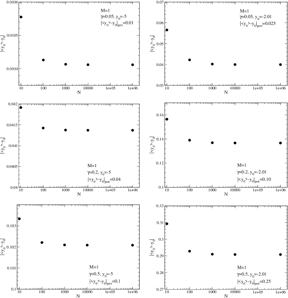
Figure 1: The shift of the single $P$–space state (M = 1) due to the coupling with $N$ $Q$–space states versus $N$ for several values of the coupling strength $\gamma$ and for two positions $y_{0}$ of the state.

We first consider the case of a one–dimensional $P$–space hosting the system’s ground state. The numerical calculation yields the end points of that part of the spectrum which is due to the presence of the $P$–space state. From here we calculate the center of the spectrum and its length. We call the difference between the unperturbed position and the center of the spectrum the shift and the length of the spectrum the fluctuation and compare both values with the perturbative estimates of Sections 3 and 5. We must keep in mind, of course, that the present definitions of shift and fluctuation differ from the ones used in Section 3.

In Fig. 1 the downward shift of the $P$–space state due to the coupling with the $N$ chaotic $Q$–space states is displayed versus $N$ for several values of the coupling strength $\gamma$. For the sake of comparison, the $N$–independent perturbative result $|\langle y_{0}\rangle-y_{0}|_{\rm pert}$ is also given in each panel. In all cases, the downward shift increases monotonically with the number $N$ of states in $Q$–space and reaches saturation at about $N=10^{4}$. In the sequel, “shift” is used for that asymptotic value.

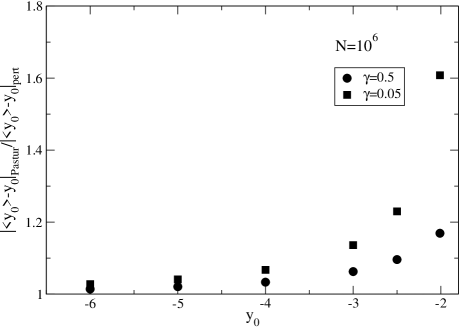
Figure 2: Ratios of exact and perturbative results for the shift for $N\gg 1$ versus distance from the centre of the semicircle.

In the Figure we display two cases:

• The $P$–space state lies far from the $Q$–space spectrum. The downward shift increases monotonically and almost exactly linearly with $\gamma$. Indeed, in going from $\gamma=0.05$ to $\gamma=0.5$ the value grows by an order of magnitude. The predictions of perturbation theory are in order and, notably, turn out to be always smaller in magnitude than the ones stemming from the generalized Pastur equation albeit by a small amount (roughly by about $4\div 6\%$ for $N$ not too large).

• The $P$–space state lies just below the semicircle. Again the shift increases monotonically with $\gamma$ but now perturbation theory badly underestimates the shift, especially for small values of $\gamma$.

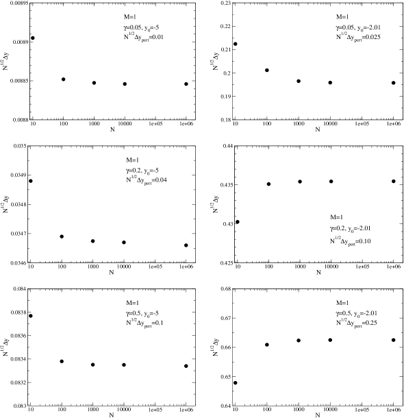
Figure 3: The fluctuation $\Delta y$ (square root of the variance) of the position of the single $P$–space state versus $N$ for several values of the coupling strength $\gamma$ and for two positions $y_{0}$ of the state. We have scaled $\Delta y$ with $N^{1/2}$.

A summary of our results is given in Fig. 2. For two values of $\gamma$, we show the ratio of the exact result over the perturbative result for the shift versus distance from the centre of the semicircle. We recall that in our units, the radius of the semicircle is two. The Figure indicates the goodness of perturbative results. For reasonable values of $\gamma\leq 1/2$, lowest–order perturbation theory furnishes reliable results if the distance of the $P$–state from the edge of the semicircle is larger than the radius of the semicircle.

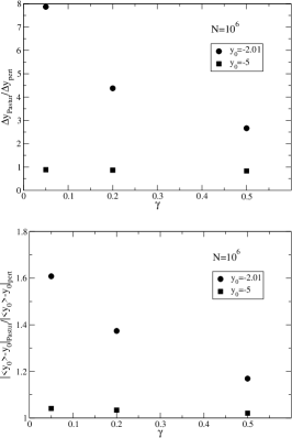
Figure 4: Ratios of exact and perturbative results for shift and fluctuation.

The fluctuations of the ground–state energy are displayed in Fig. 3. The perturbative result is also given in each panel. In all cases, the fluctuations reach saturation at about $N=10^{4}$. In the sequel, “fluctuation” is used for that asymptotic value.

• When the $P$–space state is far from the semicircle we find again that the fluctuations grow monotonically with $\gamma$, and that perturbation theory is reliable but, notably, yields results larger than the ones stemming from the Pastur equation (by about $10\div 15\%$ when $\gamma$ is small, up to about $18\%$ when $\gamma$ is large; these estimates depend, of course, upon the definition of $\Delta y$).

• Perturbation theory fails when the $P$–space state lies close to the semicircle yielding values much smaller than those inferred from the Pastur equation.

Our results are summarized in Fig. 4 where we show the ratios of the exact values over the perturbative results for the fluctuations (upper panel) and for the shifts (lower panel) versus the coupling strength $\gamma$. We observe that the discrepancy between perturbative and exact results is decreasing with increasing $\gamma$. We have no explanation for this observation.

To assess the validity of our results for realistic cases, we must address the case of $P$–spaces of dimension $>1$. We do so for a two–dimensional $P$–space. We assume that the two $P$–space states are not coupled to each other, and that both have the same average coupling to the $Q$–space states. The results for this case are displayed in Fig. 5. We show versus $N$ the average shift and the fluctuation of the lowest $P$–space state located originally at $y_{0}=-5$ for four cases: (i) $P$–space is one–dimensional (M = 1), (ii) $P$–space is two–dimensional and the second state is originally located at $y_{1}=-2.01$, (iii) $P$–space is two–dimensional and the second state is originally located at $y_{1}=-4.9$, (iv) $P$–space is two–dimensional and the second state is originally located at $y_{1}=-4.99$, i.e., in the immediate vicinity of the first state.

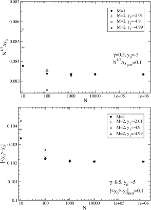
Figure 5: Influence of the induced level repulsion between two states in $P$–space on shift and fluctuation versus $N$.

We observe that the downward shift of the lower of the two $P$–space states increases as the distance to the higher $P$–space state is reduced. In fact, the shift now arises from the combined action of the coupling with the $Q$–space and the induced coupling to the other state in $P$-space. However, this effect is visible only for $N\leq 100$. For large values of $N$, the induced level repulsion between the two states in $P$–space is negligible. This is in accord with the results of Sections 3 and 5. The fluctuations also increase as the two states of the $P$-space come closer to each other but again this effect is visible only for $N\leq 100$.

6.2 Overlapping Spectra

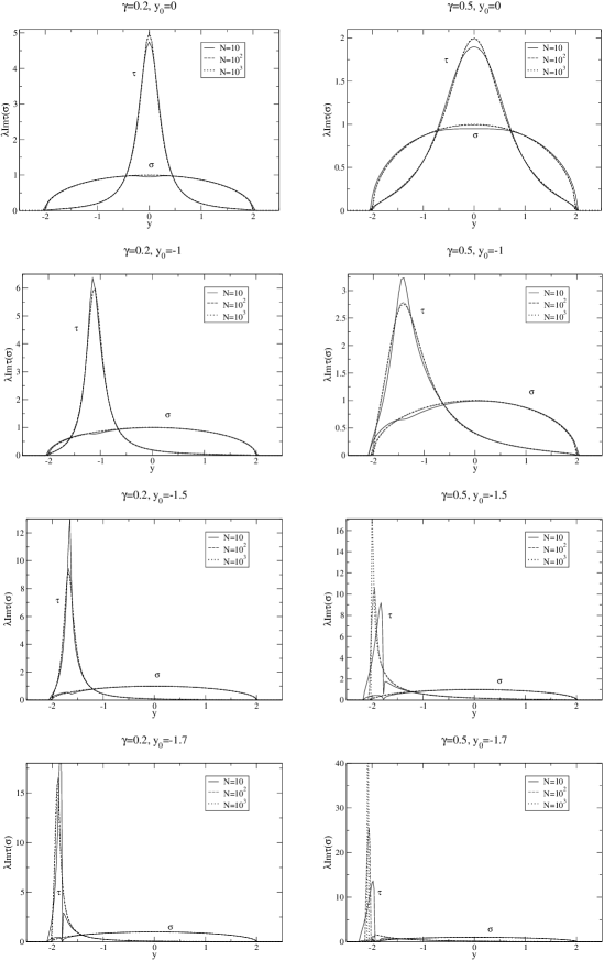
Figure 6: The imaginary parts of $\lambda\tau$ and of $\lambda\sigma$ for two different coupling strengths $\gamma$, and for several positions $y_{0}$ of the $P$–space state.

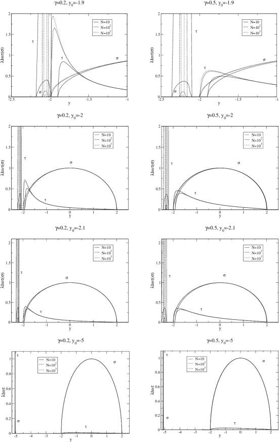
Figure 7: Same as Fig. 6 but for $y_{0}$ close to the end point of the semicircle. The four panels at the bottom show the values of $\lambda\tau$ and of $\lambda\sigma$ for the case of non–overlapping spectra.

We consider a one–dimensional $P$–space with $E_{0}$ embedded into the GOE spectrum. We display the imaginary parts of the spectral functions $\lambda\tau$ and $\lambda\sigma$ as defined in Eqs. (40) and (23). In addition we also show these two functions for the case where $E_{0}$ lies far outside the semicircle.

Figs. 6 and 7 show the imaginary parts for two values of the coupling strength $\gamma$ and for several values of the initial position $y_{0}$ of the $P$–space state. In each panel we display the results for several choices of the dimension $N$ of $Q$–space. We see that in the weak–coupling regime ($\gamma=0.2$) and for $y_{0}=0$, the $P$–space spectral function $\tau$ is well represented by a Lorentzian. As $y_{0}$ moves towards the end point of the GOE spectrum, the Lorentzian becomes increasingly distorted. With the Lorentzian normalized to $\pi$ the product of height and width (computed at half its maximum) should be 2. For the figure shown that product is larger than 2 (the more so the more $y_{0}$ approaches the center of the semicircle). As a consequence of level repulsion, the imaginary part of $\sigma$ is not confined to the interior of the original GOE semicircle. For $y_{0}$ near the center of the semicircle, the dilatation of the semicircle gets smaller, however, with increasing $N$. The situation changes when $y_{0}$ is close to the end point $-2$.

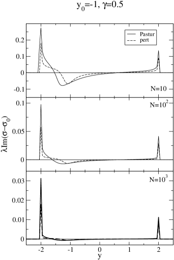
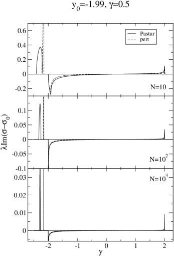
Figure 8: $\lambda{\rm Im}(\sigma-\sigma_{0})$ as obtained from the exact solution of the Pastur equation (solid line) and from the perturbative solution (55) (dashed line) for $y_{0}=-1$, $\gamma=0.5$ and several values for $N$.

Figure 9: Same as Fig. 9, but for $y_{0}=-1.99$.

In the strong–coupling regime ($\gamma=0.5$) and for $y_{0}$ near the center of the semicircle, the imaginary part of $\tau$ resembles a Gaussian more than a Lorentzian. Remarkably, the peak height is still given by $1/\gamma$, irrespective of the strength of $\gamma$. Again, the function becomes strongly distorted as $y_{0}$ approaches the end point. As a consequence of level repulsion, the total spectrum may even develop two branches although the $P$–space state originally lies within the semicircle.

It is of interest to compare the perturbative solution (55) of the Pastur equation with the exact one. For two values of $y_{0}$ (position of the $P$–state) and several values of $N$, this is done in Figs. 9 and 9. We note that for $N\gg 1$, the perturbative solution becomes amazingly accurate, even in the strong coupling limit. However, when the $P$–space state is very close to the edge of the semicircle ($y_{0}=-1.99$), perturbation theory appears to be unable to reproduce the position of the peak outside the semicircle.

We have used the exact results partly displayed in Figs. 6 and 7 to check whether the imaginary parts of $N\sigma/\pi$ and $\tau/\pi$ add up to $N+1$ as they should. We found this indeed to be the case to within about 0.1 percent. This is the expected numerical accuracy of our results. Remarkably, this outcome is valid no matter what the value of $N$: We thus conclude that Pastur equation, while missing contributions of the order of $1/N$, yet preserves the normalization of the density of states.

7 Summary and Conclusions

We have given a comprehensive treatment of the interaction between regular and chaotic states. We have modelled the latter in terms of the GOE, the Gaussian Orthogonal Ensemble of Random Matrices. Using the limit of large matrix dimension for the GOE, we have derived a generalization of the Pastur equation for the ensemble average of the Green’s function of the system. That non–perturbative equation furnishes exact results via numerical calculations. Using that approach we have shown that the coupling induced between two regular states by their interaction with the chaotic states is very small and, in fact, negligible. This is true provided both states are coupled equally strongly to the chaotic states. For that reason, we have focused attention throughout most of the paper on a single regular state interacting with a large number of chaotic states.

To gain an analytical understanding of the behavior of the system we use approximate results. To this end we employ two types of perturbation theory: Canonical perturbation theory for the secular equation for the eigenvalues of the Hamiltonian, and a perturbative treatment of the generalized Pastur equation.

We have considered two cases: The regular state lies either outside or inside the GOE spectrum. In the first case, we calculate the mean value and the variance of the shift, or another measure of its spread, as mean values over the ensemble. The two perturbative approaches yield essentially identical results and agree with the exact solution if the distance between the energy of the regular state and the end point of the GOE spectrum is sufficiently large. For realistic coupling strengths that means the distance is similar to the radius of the semicircle. Due to the interaction with the chaotic states, the spectrum of a set of regular levels will get quenched. The quenching is not uniform but grows with decreasing distance from the semicircle.

The interaction not only alters the position (and the wave function) of the regular state but also affects the shape of the GOE spectrum. The ensuing deformation is particularly relevant when the regular state lies within the GOE spectrum and close to one of its end points. The state itself gets shifted, and acquires a spreading width. Canonical perturbation theory, based on a power series expansion in the strength of the coupling between regular and chaotic states, yields estimates for these quantities. The perturbative solution to the Pastur equation does not rely on the smallness of that strength and displays a non–linear dependence of the spreading width on the strength. We believe this to be an interesting effect which does not seem to have been taken into account previously and which deserves further study. The shape of the spectrum due to the regular state is Lorentzian for small couplings and gradually changes into a Gaussian as the coupling is increased and becomes comparable to the radius of the semicircle. The shape change of the chaotic spectrum is not accessible to canonical perturbation theory but can be estimated using the modified perturbation theory for the generalized Pastur equation. Comparing the results of the latter with the exact ones, we find that the perturbative solution is excellent for $N\gg 1$. When the energy of the regular state is close to the edge of the GOE spectrum, the regular state is pushed outside the GOE spectrum as a consequence of level repulsion for sufficiently strong coupling. In that case the spectrum develops two branches. The perturbative approach is unable to account quantitatively for the part of the spectrum outside the semicircle.

In conclusion: We have derived and solved exactly the generalized Pastur equation for a complex system with strong interactions. We have shown that perturbation theory, either canonical or on the Pastur equation, is valid. We may view our dynamical system as a generic model for a complex, strongly interacting many–body system. In the light of such a view, our results are remarkable. They convey the huge simplification of the many–body problem induced by the concept of ensemble averaging.

Appendix

To calculate the shift of the unperturbed energy $E_{0}$ we have to evaluate the ensemble averages of the first and of the second term on the right–hand side of Eq. (8). For the first term we obtain

$$\left\langle\sum_{\mu=1}^{N}\frac{V_{\mu}^{2}}{E_{\mu}-E_{0}}\right\rangle={\mathcal{V}}^{2}\left\langle\sum_{\mu=1}^{N}\frac{1}{E_{\mu}-E_{0}}\right\rangle={\mathcal{V}}^{2}\int\d E\frac{1}{E-E_{0}}\sum_{\mu=1}^{N}\langle\delta(E-E_{\mu})\rangle\ .$$ (57)

The expression $\sum_{\mu=1}^{N}\langle\delta(E-E_{\mu})\rangle$ is the average level density of the GOE and given in Eq. (9). With the dimensionless variables $x=E/2\lambda$ and $x_{0}=E_{0}/2\lambda$ we get

$$\left\langle\sum_{\mu=1}^{N}\frac{V_{\mu}^{2}}{E_{\mu}-E_{0}}\right\rangle=\frac{{\mathcal{V}}^{2}N}{\pi\lambda}I(x_{0})$$ (58)

where $I(x_{0})$ is defined in Eq. (12). As for the second term on the right–hand side of Eq. (8), we keep only the leading contributions in an expansion in inverse powers of $N$. Thus, in the identity $\langle V_{\mu}^{2}V_{\nu}^{2}\rangle=({\mathcal{V}}^{2})^{2}(1+2\delta_{\mu\nu})$ the contribution from the Kronecker delta is negligible. Averaging over the $V_{\mu}$’s yields

$$\left\langle\sum_{\mu=1}^{N}\frac{V_{\mu}^{2}}{E_{\mu}-E_{0}}\sum_{\nu=1}^{N}\frac{V_{\nu}^{2}}{(E_{\nu}-E_{0})^{2}}\right\rangle=({\mathcal{V}}^{2})^{2}\left\langle\sum_{\mu=1}^{N}\frac{1}{E_{\mu}-E_{0}}\sum_{\nu=1}^{N}\frac{1}{(E_{\nu}-E_{0})^{2}}\right\rangle.$$ (59)

The two–level correlation function decreases as a Bessel function over distances large with respect to the level spacing $d$, but small with respect to $\lambda\approx Nd$ [7] and can be neglected in a calculation keeping only the leading order in $1/N$. Thus we get

$$\left\langle\sum_{\mu=1}^{N}\frac{V_{\mu}^{2}}{E_{\mu}-E_{0}}\sum_{\nu=1}^{N}\frac{V_{\nu}^{2}}{(E_{\nu}-E_{0})^{2}}\right\rangle=\frac{({\mathcal{V}}^{2})^{2}N^{2}}{2\pi^{2}\lambda^{3}}I(x_{0})\frac{\d I(x_{0})}{\d x_{0}}\ .$$ (60)

For the shift this gives Eq. (11). The variance of $\delta\alpha$ is obtained similarly.

References

- [1] T. Guhr, A. Müller-Groeling and H. A. Weidenmüller, Phys. Rep. 299 (1998) 189.
- [2] A. Bohr and B. Mottelson, Nuclear Structure, Benjamin, New York, 1969, Vol. 1.
- [3] C. Mahaux and H. A. Weidenmüller, Shell–Model Approach to Nuclear Reactions, North–Holland, Amsterdam, 1969.
- [4] H. Feshbach, Theoretical Nuclear Physics: Nuclear Reactions, Wiley-Interscience, New York, 1992.
- [5] H. Feshbach, Phys. Rep. 264 (1996) 13; R. Caracciolo, A. De Pace, H. Feshbach and A. Molinari, Ann. Phys. (N.Y.) 262 (1998) 105; A. De Pace, H. Feshbach and A. Molinari, Ann. Phys. (N.Y.) 278 (1999) 109; A. De Pace and A. Molinari, Ann. Phys. (N.Y.) 296 (2002) 263.
- [6] A. Molinari and H. A. Weidenmüller, Phys. Lett. B 601 (2004) 119; ibid., 637 (2006) 48.
- [7] K. B. Efetov, Supersymmetry in Disorder and Chaos, Cambridge University Press, Cambridge, 1997.