Landau parameters for isospin asymmetric nuclear matter based on a relativistic model of composite and finite extension nucleons

Abstract

We study the properties of cold asymmetric nuclear matter at high density, applying the quark meson coupling model with excluded volume corrections in the framework of the Landau theory of relativistic Fermi liquids. We discuss the role of the finite spatial extension of composite baryons on dynamical and statistical properties such as the Landau parameters, the compressibility, and the symmetry energy. We have also calculated the low lying collective eigenfrequencies arising from the collisionless quasiparticle transport equation, considering both unstable and stable modes. An overall analysis of the excluded volume correlations on the collective properties is performed.

PACS : 12.39.Ba, 21.30.Fe, 21.65.+f, 71.10.Ay

1 Introduction

The study of the nuclear medium composed of different fractions of protons and neutrons has been developed for long time and it has concentrated a renewed interest in the last years. The equation of state of isospin asymmetric nuclear matter is a subject of particularly intense research [1, 2, 3, 4, 5]. The possible applications range from the structure of radiative nuclei, the dynamics of rare isotopes and the cooling process of neutron stars. A key role in many of these calculations is played by the density dependence of the symmetry energy [3], which may be extracted from recent isospin diffusion data in heavy ion collisions experiences [2].
The standard theoretical calculations have used as the relevant degrees of freedom protons and neutrons, moving non-relativistically through potentials representing the averaged instantaneous interaction among nucleons. Furthermore, since the development of the Quantum Hadro-Dynamics [6], it has became a common practice to use relativistic hadronic fields in these kind of calculations. In such a case the nuclear interaction is mediated by mesons of scalar or vector isospin character. The role of the scalar isovector meson ($a_{0}$ (980)) has been emphasized in recent investigations [7].

A further step has been given by models incorporating the quark structure of hadrons. They may be reduced to mean field hadronic pictures whose parameters, such as masses and vertices, hide the quark dynamics. These effective models provide both a connection between the hadronic phenomenology and the fundamental theory of the strong interactions, besides a sound description of hadronic matter and atomic nuclei.

Among the dual quark-hadron theoretical frameworks, those based on the bag models include explicitly the quark confinement volume. Specifically, the Quark Meson Coupling (QMC) [8] states the dynamical evolution of this confining region, which depends on the global properties of the nuclear medium as well as on the configuration of the hadronic fields. However, this feature is usually missed [8] in passing to a pure hadronic context, as baryons and mesons are regarded as point-like particles in this limit.
The relevance of the finite extension of nucleons in the evaluation of some nuclear statistical properties has been stressed long time ago [9]. In order to fulfill this assertion, several corrections have been introduced in the hadronic interactions, mainly invoking a Van der Waals-like normalization [10, 11, 12, 13]. The motivation for such a procedure is to parameterize in compact form the strong baryon-baryon repulsion at very short distances. In the high density realm of nuclear matter the mean free path of nucleons is comparable to the quark confining size, hence excluded volume effects become relevant.
The correction due to the finite extension of nucleons have been introduced into the hadronic sector of the bag models [12, 13], it was found that it is necessary to describe properly high density hadronic matter without violating the model assumptions [13].

Another theoretical scheme suitable to describe the nuclear collective phenomena is the Landau theory of Fermi liquids. Although it was originally stated in a non-relativistic fashion, see for instance [14], it was subsequently extended to deal with the relativistic fields formalism [15, 16]. The Landau parameters are useful to evaluate thermodynamical properties, the stability conditions in phase transitions, the nuclear matter collective excitations which couple, for instance, to the weak interaction governing the neutrino emission of URCA processes in neutron stars.

In this work the behaviour of isospin asymmetric nuclear matter is studied in the framework of the QMC model with excluded volume corrections in the hadronic sector. Special attention is paid to the Landau parameters and the collective modes. In the next section we give a resume of the QMC model and we describe the correlations generated by the Van der Waals-like normalization. In section 3 we define the Landau parameters and use them in section 4 to derive the isoscalar and isovector collective modes. Results and discussions are presented in section 5, and finally the conclusions are drawn in section 6.

2 The Quark Meson Coupling Model

QMC is an effective model of the quark structure of hadrons, it is inspired in the MIT bag model, so that in its starting point the confinement mechanism has being accomplished and chiral symmetry has been broken. In order to describe the dynamics of the emerging hadrons, usually the model is projected into a picture of point-like baryons interacting through virtual mesons [8], the same ones which couple quarks inside the confinement region. Since we are primarily concerned with isospin asymmetric nuclear matter, we only consider $u$ and $d$ flavor of quarks coupled by the isovector $\rho$ and $\delta$ ($a_{0}$ (980)) mesons, besides the commonly used iso-scalar $\sigma$ and $\omega$ ones.
Within the QMC model baryons are represented as non-overlapping spherical bags containing three valence quarks; the bag radius changes dynamically with the fields configuration.
The mean field approximation (MFA) is the natural scheme of solution, which replaces the meson fields by its classical expectation values. These mean values determine the nucleon fields, which in turn become the source of the meson ones.
In the MFA the Dirac equation for a quark of flavor $q,\;(q=u,d)$, of current mass $m_{q}$ and $I_{q}$ third isospin component, is given by [8]

$$(i\gamma^{\mu}\partial_{\mu}-g_{\omega}^{q}\gamma^{0}\omega-g_{\rho}^{q}I_{q}\;\gamma^{0}\rho-{m_{q}}^{\ast})\Psi^{q}=0,$$ (2.1)

here the notation ${m_{q}}^{\ast}=m_{q}-g_{\sigma}^{q}\sigma-I_{q}g_{\delta}^{q}\delta$ is used.
For a spherically symmetric bag of radius $R_{b}$ corresponding to a baryon of class $b$, the normalized quark wave function $\Psi^{q}_{b}(r,t)$ is given by

$$\Psi^{q}_{b}(r,t)={\cal N}_{b}^{-1/2}\frac{e^{-i{\varepsilon}_{qb}t}}{\sqrt{4\pi}}\left(\begin{array}[]{c}j_{0}(x_{qb}\,r/R_{b})\\ i\beta_{qb}{\vec{\sigma}}.{\hat{r}}j_{1}(x_{qb}\,r/R_{b})\end{array}\right)\chi^{q},$$ (2.2)

where $\chi^{q}$ is the quark spinor and

$$\varepsilon_{qb}=\frac{\Omega_{qb}}{\!R_{b}}+g_{\omega}^{q}\;\omega+g_{\rho}^{q}I_{q}\;\rho,$$ (2.3)

$${\cal N}_{b}={R_{b}}^{3}\;[2\Omega_{qb}(\Omega_{qb}-1)+R_{b}{m_{q}}^{\ast}]\;\frac{j_{0}^{2}(x_{qb})}{x_{qb}^{2}},$$ (2.4)

$$\beta_{qb}={\left[\frac{\Omega_{qb}-R_{b}{m_{q}}^{\ast}}{\Omega_{qb}+R_{b}{m_{q}}^{\ast}}\right]}^{1/2},$$ (2.5)

with $\Omega_{qb}=[x_{qb}^{2}+{(R_{b}{m_{q}}^{\ast})}^{2}]^{1/2}$. The eigenvalue $x_{qb}$ is the lowest solution of the equation

$$j_{0}(x_{qb})=\beta_{qb}\;j_{1}(x_{qb}),$$ (2.6)

which arises from the boundary condition at the bag surface.
In this model the ground state bag energy is identified with the baryonic mass $M_{b}$,

$$M_{b}=\frac{\sum_{q}n_{q}^{b}\Omega_{qb}-z_{0b}}{R_{b}}+\frac{4}{3}\pi B_{0}{R_{b}}^{3},$$ (2.7)

where $n_{q}^{b}$ is the number of quarks of flavor $q$ inside the bag. The bag constant $B_{0}$ is numerically adjusted to get definite values for the proton bag radius, and the zero-point motion parameters $z_{0b}$ are fixed to reproduce the baryon spectrum at zero density.
The dispersion relation for the b-baryon is

$$k_{0}^{b}=\sqrt{{M_{b}}^{2}+(\mathbf{k}-\mathbf{\Sigma}_{b})^{2}}\pm g_{\omega}\omega_{0}\pm g_{\rho}I_{b}\rho_{0}^{3},$$ (2.8)

for particle $(+)$ and antiparticle $(-)$ solutions. Within the MFA at zero temperature only the particle solutions contribute. In this expression we have assumed that the strength of the couplings does not depend on the quark flavor. We have also introduced the baryonic isospin projection $I_{b}=\sum_{q}n_{q}^{b}I_{q}$, and the vector nucleon selfenergy $\mathbf{\Sigma}_{b}=g_{\omega}\mathbf{\omega}+g_{\rho}\mathbf{\rho}I_{b}$.

For homogeneous infinite static matter the spatial dependence of all the meson fields can be neglected, so that its equations of motion reduce in the MFA to

$$\sigma = =-\frac{1}{{m_{\sigma}}^{2}}\sum_{b}\left(\frac{\partial M_{b}}{\partial\sigma}\right)_{R,\delta}n_{s}^{b},$$ (2.9)

$$\omega_{\mu} = \frac{1}{{m_{\omega}}^{2}}\sum_{b}g_{\omega}j_{\mu}^{\;b},$$ (2.10)

$$\delta = -\frac{1}{{m_{\delta}}^{2}}\sum_{b}\left(\frac{\partial M_{b}}{\partial\delta}\right)_{R,\sigma}n_{s}^{b},$$ (2.11)

$$\rho_{\mu} = \frac{1}{{m_{\rho}}^{2}}\sum_{b}g_{\rho}I_{b}j_{\mu}^{\;b}.$$ (2.12)

Here $j_{\mu}^{\,b}=(n^{b},\mathbf{j}^{\;b})$ stands for the mean value of the nucleon current density of isospin $b$. In the reference frame where the averaged momentum of matter is zero the spatial components of the currents become null $\mathbf{j}^{\;b}=0$, hence only the time-like projections of the vector mesons are non-zero.
It must be noted that Eqs. (2.11) and (2.12) refer only to the third isospin component, since the remaining ones become zero in the MFA.

From the relations (2.7) and (2.8) it can be seen, as it was earlier mentioned, that the nucleon mass and energy spectrum depends on the assumed meson classical values. They are in turn, determined by the nucleon densities as given by the equations (2.9)-(2.12).

The densities $n_{s}^{b}$ and $j_{\mu}^{\;b}$ are defined with respect to the ground state of the hadronic matter, which at zero temperature is composed of baryons filling the Fermi sea up to the state with momentum $k_{Fb}$

$$n_{s}^{b} = \;\frac{\vartheta}{(2\pi)^{3}}\sum_{spin}\int\frac{d^{3}k\;M_{b}}{\sqrt{{M_{b}}^{2}+(\mathbf{k}-\mathbf{\Sigma}_{b})^{2}}}\;\theta(k_{Fb}-|\mathbf{k}|),$$ (2.13)

$$j_{\mu}^{\;b} = \;\frac{\vartheta}{(2\pi)^{3}}\sum_{spin}\int\frac{d^{3}k\;(k-\Sigma)_{\mu}}{\sqrt{{M_{b}}^{2}+(\mathbf{k}-\mathbf{\Sigma}_{b})^{2}}}\;\theta(k_{Fb}-|\mathbf{k}|).$$ (2.14)

In Eqs. (2.13) and (2.14 ) the factor $\vartheta$ is included for future use and it takes the value $\vartheta=1$ for point-like baryons.

The total energy density $\mathcal{E}$ and pressure $P_{0}$ of hadronic matter for point-like baryons is evaluated as

$$\mathcal{E} = \frac{1}{2}m_{\sigma}^{2}\;\sigma^{2}+\frac{1}{2}m_{\omega}^{2}\;\omega^{2}+\frac{1}{2}m_{\rho}^{2}\;\rho^{2}+\frac{1}{2}m_{\delta}^{2}\;\delta^{2}$$ (2.15)

$$+ \frac{\vartheta}{{\pi}^{2}}\sum_{b}\int_{0}^{k_{Fb}}dkk^{2}\sqrt{{M_{b}}^{2}+k^{2}},$$

$$P_{0} = \sum_{b}\mu_{0}^{b}n^{b}-\mathcal{E},$$ (2.16)

where $\mu_{0}^{b}=k_{0}^{b}(k_{Fb})$, see Eq. (2.8), is the chemical potential for point-like baryons.

In the QMC the radius $R_{b}$ is a variable dynamically adjusted to reach the equilibrium of the bag in the dense hadronic medium. We use the equilibrium condition proposed in ref. [13], which can be obtained by minimizing the energy density $\mathcal{E}$ with respect to $R_{b}$

$$-\frac{1}{4\pi R_{b}^{2}}{\left(\frac{\partial{M_{b}}}{\partial R_{b}}\right)}_{\sigma,x_{qb}}=\frac{1}{3{\pi}^{2}\,\xi}\sum_{c}\int_{0}^{k_{Fc}}\frac{dkk^{4}}{\sqrt{{M_{c}}^{2}+k^{2}}},$$ (2.17)

where $\xi=1$. This result reflects the balance of the internal pressure of the bag with the baryonic contribution to the total external pressure, represented by the left and right sides of Eq.(2.17), respectively.
The factor $\xi$ will be redefined below where excluded volume effects will be considered.

The QMC model heavily relies on the assumption of non-overlapping bags, using this criterion an upper density limit around three times the saturation density of symmetric nuclear matter has been found [17]. In order to properly take into account this severe restriction, a simplified model was introduced in [13], which describe baryons as extended objects. Since finite size baryons are assumed non-overlapping, their motion must be restricted to the available space $V^{\prime}$ defined as [10]

$$V^{\prime}=V-\sum_{b}N^{b}v_{b},$$ (2.18)

with $N^{b}$ the total number of baryons of class $b$ inside the volume $V$, and $v_{b}$ the effective volume per baryon of this class. The last mentioned quantity is proportional to the actual baryon volume, i.e. for spherical volumes of radius $R_{b}$

$$v_{b}=\alpha\frac{4\pi}{3}{R_{b}}^{3},$$ (2.19)

where $\alpha$ is a real number ranging from $4$, in the low density limit, to $3\sqrt{2}/{\pi}$, which corresponds to the maximum density allowed for non overlapping spheres, in a face centered cubic arrange. Since we wish to study the high density regime of homogeneous isotropic matter, we shall adopt $\alpha=3\sqrt{2}/{\pi}$ in all our calculations.

Consequently it was assumed that the nucleon fields can be normalized replacing $V^{\prime}$ for $V$, which in turn implies a normalization of the nucleon densities (2.13), (2.14) and of the nucleon contribution to the energy (2.15). The final result may be obtained by taking $\vartheta=1-\sum_{b}n^{b}v_{b}$ within these equations and $\xi={n^{b}_{s}}/{(\alpha\,n^{b})}$ in Eq. (2.17) [13].

Since $\vartheta$ introduces an explicit dependence upon the baryonic densities, the chemical potentials get an extra term, i.e.

$$\mu^{b} = {\left(\frac{\partial\mathcal{E}}{\partial n_{b}}\right)}_{{n_{{b^{\prime}}_{{}_{{}_{{}_{\!\!\!\!\!\!\!\!\!\!\!b^{\prime}\neq b}}}}}}}=\mu_{0}^{b}+\Delta\mu^{b},$$ (2.20)

$$\Delta\mu^{b} = \frac{v_{b}}{3{\pi}^{2}}\sum_{c}\int_{0}^{k_{Fc}}\frac{dkk^{4}}{\sqrt{{M_{c}}^{2}+k^{2}}}.$$ (2.21)

Correspondingly, the total pressure acquires an additional term $\Delta P$ as compared to the pressure of point-like baryons $P_{0}$ in Eq. (2.16)

$$P_{H}=P_{0}+\Delta P=P_{0}+\sum\limits_{b}n^{b}\Delta\mu^{b}.$$ (2.22)

3 Landau parameters and equation of state

The Fermi liquid theory of Landau assumes that the low-lying excitations of a physical system admits a representation in terms of quasi-particles and, circumstantially, collective modes. If the quasi-particle states can be identified by a composed label $B=(b,\beta)$, where we have singled out the first place for the isospin projection and $\beta$ collects discrete spin and momentum indices, then the occupation number of such a level is denoted by $f_{B}$. The conserved baryonic number can be expressed in terms of a summation over such distribution functions: $n=\sum_{B}f_{B}$. The same statement is valid for every extensive conserved quantity such as the energy, which can be written as $\sum_{B}\,f_{B}\varepsilon_{B}$ plus current-current interactions, where $\varepsilon_{B}$ is the nucleon single particle spectrum. For infinite nuclear matter the summation over the discrete momentum indices must be replaced by an integration over the continuous spectrum with measure $d^{3}k/(2\pi^{3})$.
The formulae (2.13) and (2.14) for the nucleon densities must be rewritten in order to fit this form. Firstly the replacement $p_{i}=k_{i}\,\vartheta^{1/3}$ is made, secondly we identify $\sum_{spin}\int d^{3}p\;\theta(p_{Fb}-|\mathbf{p}|)/(2\pi)^{3}\rightarrow\sum_{\beta}f_{b\,\beta}$, with $p_{Fb}=k_{Fb}\,\vartheta^{1/3}$. Hence, Eqs. (2.13), (2.14), and (2.15) can be rewritten as

$$n_{s}^{b} = \sum_{\beta}\frac{f_{b\,\beta}\,M_{b}}{\sqrt{M_{b}^{2}+(\vartheta^{-1/3}\mathbf{p}_{\beta}-\mathbf{\Sigma}_{b})^{2}}},$$ (3.1)

$$j_{\mu}^{\;b} = \sum_{\beta}\frac{f_{b\,\beta}\,(\vartheta^{-1/3}p_{\beta}-\Sigma_{b})_{\mu}}{\sqrt{M_{b}^{2}+(\vartheta^{-1/3}\mathbf{p}_{\beta}-\mathbf{\Sigma}_{b})^{2}}},$$ (3.2)

$$\mathcal{E} = \sum_{B}f_{b\,\beta}\left(\sqrt{M_{b}^{2}+(\vartheta^{-1/3}\mathbf{p}_{\beta}-\mathbf{\Sigma}_{b})^{2}}+g_{\omega}\,\omega_{0}+I_{b}g_{\rho}\rho_{0}\right)$$ (3.3)

$$+\frac{1}{2}\left(m_{\sigma}^{2}\,\sigma^{2}+m_{\delta}^{2}\,\delta^{2}-m_{\omega}^{2}\,\omega_{\mu}\omega^{\mu}-m_{\rho}^{2}\,\rho_{\mu}\rho^{\mu}\right),$$

where the momentum independence of the nucleon masses, characteristic of the Hartree approximation, has been emphasized.
In the last formula $\mathcal{E}$ must be considered as a function of the distribution functions $f_{B}$, the bag radii $R_{b}$ and the meson fields $\phi=\sigma,\,\omega,\,\delta,\,\rho$, hence first variation of the energy density yields

$$\delta\mathcal{E}(f,R,\phi)=\sum_{b}\frac{\partial\mathcal{E}}{\partial R_{b}}\delta R_{b}+\sum_{\phi}\frac{\partial\mathcal{E}}{\partial\phi}\delta\phi+\sum_{B}\frac{\partial\mathcal{E}}{\partial f_{B}}\,\delta f_{B}.$$

The first term is null because of the equilibrium condition for the bag in the nuclear medium, Eq. (2.17), the second one is likewise zero due to the meson field equations (2.9)-(2.12). Therefore, the quasiparticle energy spectrum according to the Fermi liquid prescription is

$$\varepsilon_{B} = \frac{\partial\mathcal{E}}{\partial f_{B}}=\sqrt{M_{b}^{2}+(\vartheta^{-1/3}\mathbf{p}_{\beta}-\mathbf{\Sigma}_{b})^{2}}+g_{\omega}\omega_{0}+g_{\rho}\rho_{0}I_{b}$$ (3.4)

$$+\frac{v_{b}}{3}\sum_{B^{\prime}}f_{B^{\prime}}\frac{\vartheta^{-4/3}\mathbf{p}_{\beta^{\prime}}\cdot\left(\vartheta^{-1/3}\mathbf{p}_{\beta^{\prime}}-\mathbf{\Sigma}_{b^{\prime}}\right)}{\sqrt{M_{b^{\prime}}^{2}+(\vartheta^{-1/3}\mathbf{p}_{\beta^{\prime}}-\mathbf{\Sigma}_{b^{\prime}})^{2}}}.$$

If Eq. (3.4) is evaluated at the Fermi surface, i.e. $|\mathbf{p}_{\beta}|=p_{\beta}=p_{Fb}$, in the limit of isotropic matter and restoring the continuum spectrum, it yields the chemical potential given by Eqs. (2.20), (2.21), in support of the thermodynamical consistency of our approach.

In order to evaluate the Landau’s parameters of the nuclear interaction, a second variation must be performed, i.e. $F_{B^{\prime}\,B}=\partial^{2}\mathcal{E}/\partial f_{B^{\prime}}\,\partial f_{B}=F_{B\,B^{\prime}}$. Since all of the bag radii and the meson fields depend ultimately on the distribution functions $f_{B}$, Eqs. (2.9)-(2.12) and (2.17) must be differentiated in order to obtain a closed expression.
The Landau’s parameters are defined as the Fourier coefficients of an expansion in terms of the Legendre polynomials

$$F^{l}_{BB^{\prime}}=(l+1/2)\int_{-1}^{1}dx\,P_{l}(x)\,\frac{\partial^{2}\mathcal{E}(x)}{\partial f_{B^{\prime}}\,\partial f_{B}},$$

where the integrand must be evaluated on the Fermi surface at the end of the calculations.
It is found that the second order derivative in the expression above, depends linearly on the variable $x=\mathbf{p}_{\beta^{\prime}}\cdot\mathbf{p}_{\beta}/(p_{\beta^{\prime}}\,p_{\beta})$, hence all the parameters of order greater than one are null, whereas for $l=0,\,1$ we have

$$F_{ab}^{0} = C_{\omega}+I_{a}I_{b}C_{\rho}+\sum_{c=n,p}\frac{n_{c}v_{c}}{3\vartheta R_{c}}\left(3\frac{k_{Fa}^{2}}{E_{a}}+v_{a}H^{(3)}+v_{a}\vartheta H^{(1)}H_{c}^{(2)}\frac{M_{c}}{n_{sc}}\right)X_{cb}$$ (3.5)

$$+\frac{1}{3\vartheta}\left(\frac{k_{Fa}^{2}}{E_{a}}v_{b}+\frac{k_{Fb}^{2}}{E_{b}}v_{a}\right)+\frac{v_{a}}{R_{a}}\left(1-\frac{n_{a}}{n_{sa}}\frac{M_{a}}{E_{a}}\right)H^{(1)}X_{ab}$$

$$+v_{a}v_{b}\frac{H^{(3)}}{9\vartheta}+\sum_{q=u,d}\left(n_{a}^{q}Q_{qa}\frac{M_{a}}{E_{a}}-\frac{v_{a}}{3}\sum_{c=n,p}n_{c}^{q}Q_{qc}M_{c}H_{c}^{(2)}\right)Y_{qb},$$

$$F_{ab}^{1} = -\frac{k_{a}k_{b}}{E_{a}E_{b}}\;\frac{C_{\omega}+I_{a}I_{b}C_{\rho}+2C_{\omega}C_{\rho}(1+I_{a}I_{b})n_{\overline{a}}/E_{\overline{a}}}{1+(C_{\omega}+C_{\rho})\sum_{c=p,n}\frac{n_{c}}{E_{c}}+4C_{\omega}C_{\rho}\frac{n_{1}n_{2}}{E_{1}E_{2}}}.$$ (3.6)

Here the definitions $C_{\phi}=(g_{\phi}/m_{\phi})^{2}$ for $\phi=\omega,\,\rho$ and $E_{a}=\sqrt{M_{a}^{2}+k_{Fa}^{2}}$, have been used, together with

$$H_{a}^{(1)}=\int_{0}^{k_{Fa}}\frac{dkk^{4}}{\pi^{2}\left(M_{c}^{2}+k^{2}\right)^{1/2}}, H_{a}^{(3)}=\frac{k_{Fa}^{5}}{\pi^{2}E_{a}}$$

$$H_{a}^{(2)}=\int_{0}^{k_{Fa}}\frac{dkk^{4}}{\pi^{2}\left(M_{c}^{2}+k^{2}\right)^{3/2}}, H^{(l)}=\sum_{c=p,n}H_{c}^{(l)},\,l=1,2,3$$

$$Q_{q\,a}=\frac{\Omega_{qa}+2{m_{q}}^{\ast}R_{a}\left(\Omega_{qa}-1\right)}{{m_{q}}^{\ast}R_{a}+2\Omega_{qa}\left(\Omega_{qa}-1\right)}.$$

Furthermore, the variables $X_{ab}$ and $Y_{qb}$ are the derivatives $X_{ab}=\partial R_{a}/\partial f_{B}$ and $Y_{qb}=\partial{m_{q}}^{\ast}/\partial f_{B}$ evaluated in the isotropic matter limit and taking all the momenta at the Fermi surface. Actually, they are the solutions of an algebraic coupled system of equations obtained by differentiating Eqs. (2.17), (2.9), and (2.11) and making a linear combination of the two last results.
For further development, we define symmetric adimensional Landau parameters

$$\mathcal{F}_{a\,b}^{l}=\mathcal{F}_{b\,a}^{l}=\sqrt{\Gamma_{a}\,\Gamma_{b}}\,F_{a\,b}^{l}$$ (3.7)

where $\Gamma_{b}=(k_{Fb}E_{b}/\pi^{2})\,(b=p,n)$ is the relativistic quasiparticle density of states at the Fermi surface.
Eqs. (3.5)and (3.6) coincide with the previous results [15, 16] for symmetric nuclear matter if the limit $v_{a}\rightarrow 0$ is taken carefully.

The Landau parameters can be related with the nuclear compressibility $\kappa$ and symmetry energy $E_{s}$. For a given nucleon density $n=n^{n}+n^{p}$ and asymmetry coefficient $t=(n^{n}-n^{p})/n$, it can be shown that

$$\kappa=9\,n\,{\left(\frac{\partial^{2}\mathcal{E}}{{\partial n}^{2}}\right)}_{t}=\frac{9\,n}{4}\left[\frac{{(1-t)}^{2}}{\Gamma_{p}}+\frac{{(1+t)}^{2}}{\Gamma_{n}}\right]\left(\frac{1}{\vartheta}+\mathcal{F}_{t}^{0}\right)$$ (3.8)

and

$$\frac{1}{2\,n}\,{\left(\frac{\partial^{2}\mathcal{E}}{{\partial t}^{2}}\right)}_{n}=\frac{n}{8}\left(\frac{1}{\Gamma_{p}}+\frac{1}{\Gamma_{n}}\right)\left(\frac{1}{\vartheta}+\mathcal{F}_{s}^{0}\right)$$ (3.9)

where the effective Landau parameters $\mathcal{F}_{t}^{0}$ and $\mathcal{F}_{s}^{0}$ are, respectively

$$\mathcal{F}_{t}^{0} = \frac{{(1-t)}^{2}\,\Gamma_{n}\,\mathcal{F}_{p\,p}^{0}+2\,(1-t^{2})\,\sqrt{\Gamma_{p}\,\Gamma_{n}}\,\mathcal{F}_{p\,n}^{0}+{(1+t)}^{2}\,\Gamma_{p}\,\mathcal{F}_{n\,n}^{0}}{{(1-t)}^{2}\,\Gamma_{n}+{(1+t)}^{2}\,\Gamma_{p}}$$

$$\mathcal{F}_{s}^{0} = \frac{\Gamma_{n}\,\mathcal{F}_{p\,p}^{0}-2\,\sqrt{\Gamma_{p}\,\Gamma_{n}}\,\mathcal{F}_{p\,n}^{0}+\Gamma_{p}\,\mathcal{F}_{n\,n}^{0}}{\Gamma_{n}+\Gamma_{p}}$$ (3.10)

The symmetry energy $E_{s}(n)$ is obtained from Eq.(3.9) in the limit of $t=0$. These expressions reduce to the usual ones in the symmetric case without volume corrections ($\vartheta=1$), see for instance [15, 16].

4 Collective excitations

Collective modes are associated to local density fluctuations that propagate in the hadronic mean field. These fluctuations are the effect of small perturbations of the occupation distribution $f_{B}$ around the nucleon Fermi level of the quasiparticles. At zero temperature the unperturbed nucleon distributions are given by [14]

$$f_{B}=\frac{1}{V}\,\theta(\mu_{b}-\varepsilon_{B})$$ (4.1)

where $V$ is the volume of the system, and $\mu_{b}$ is the chemical potential. Local density fluctuations add a small variation of the occupation numbers around the $f_{B}$ equilibrium value, i.e. [14, 15]

$$f_{B}(\mathbf{r},t)=f_{B}+\delta f_{B}(\mathbf{r},t)=f_{B}+\delta_{p_{\beta}\,p_{Fb}}\,u_{b}\,e^{i\,(\mathbf{q}.\mathbf{r}-\omega\,t)}$$ (4.2)

and to first order the quasiparticle energies $\varepsilon_{B}$ change accordingly

$$\delta\varepsilon_{B}(\mathbf{r},t)=\sum_{B^{\prime}}F_{B\,B^{\prime}}\,\delta f_{B^{\prime}}(\mathbf{r},t)$$ (4.3)

The propagation of these perturbations at low temperature is governed by the collisionless Landau’s kinetic equation

$$\frac{\partial f_{B}}{\partial t}+\frac{\partial f_{B}}{\partial\mathbf{r}}\,\frac{\partial\varepsilon_{B}}{\partial{\mathbf{p}}_{\beta}}-\frac{\partial f_{B}}{\partial{\mathbf{p}}_{\beta}}\,\frac{\partial\varepsilon_{B}}{\partial\mathbf{r}}=0$$ (4.4)

Introducing Eq. (4.2) into Eq. (4.4) and keeping only linear contributions of the fluctuations, we obtain

$$\frac{\partial\delta f_{B}}{\partial t}+\frac{\partial\delta f_{B}}{\partial\mathbf{r}}\,\frac{\partial\varepsilon_{B}}{\partial{\mathbf{p}}_{\beta}}-\frac{\partial f_{B}}{\partial{\mathbf{p}}_{\beta}}\,\frac{\partial\delta\varepsilon_{B}}{\partial\mathbf{r}}=0$$ (4.5)

which can be further reduced to

$$\left[\omega-\vartheta^{-2/3}\,\frac{({\mathbf{p}}_{Fb}\,.\mathbf{q}\,)}{E_{b}}\right]u_{b}-\frac{p_{Fb}}{\pi^{2}}\,({\mathbf{p}}_{Fb}\,.\mathbf{q}\,)\,\sum_{a=p,n}F_{b\,a}\,u_{a}=0.$$ (4.6)

The sum should be done at the Fermi surface of protons and neutrons. For isotropic matter the direction of propagation can be arbitrarily choosen along the azymuthal axis, so that $({\mathbf{p}}_{Fb}\,.\mathbf{q}\,)={p}_{Fb}\;q\;cos\chi_{b}$. Expanding the amplitudes $u_{b}$ and the Landau parameters $F_{b\,a}$ in terms of Legendre polynomials

$$u_{b} = \sum_{l}\,u_{b}^{l}\,P_{l}\left(\mbox{cos}\,\chi_{b}\right)$$

$$F_{b\,a}^{l} = (2l+1)\int\frac{d\Omega_{a}}{4\,\pi}\,F_{b\,a}\,P_{l}\left(\mbox{cos}(\chi_{a}-\chi_{b})\right)$$ (4.7)

and making use of the addition theorem for Legendre polynomials, we have

$$\sum_{a=p,n}F_{b\,a}\,u_{a}=\sum_{a=p,n}\,\sum_{l}\,\frac{1}{(2l+1)}F_{b\,a}^{l}\,u_{a}^{l}\,P_{l}\left(\mbox{cos}\,\chi_{b}\right)$$ (4.8)

Replacing in Eq. (4.6) and writing all back in terms of the Fermi momenta $k_{Fb}$, we arrive to the following system of homogeneus linear equations

$$\frac{u_{b}^{l}}{(2l+1)}+\vartheta\,\sum_{a=p,n}\,\sqrt{\frac{\Gamma_{b}}{\Gamma_{a}}}\,\sum_{l^{\prime}}\,\frac{1}{(2l^{\prime}+1)}\mathcal{F}_{b\,a}^{l^{\prime}}\,u_{a}^{l^{\prime}}\,\Omega_{l\,l^{\prime}}(s_{b})=0$$ (4.9)

with $s_{b}=\vartheta^{1/3}\,(\omega/q)/v_{Fb}$, where $v_{Fb}=(k_{Fb}/E_{b})$ is the relativistic quasiparticle Fermi velocity. The function $\Omega_{l\,l^{\prime}}$ is given by

$$\Omega_{l\;l^{\prime}}(s)=\Omega_{l^{\prime}\,l}(s)=\frac{1}{2}\int_{-1}^{\;\;1}dy\,P_{l}(y)\,\frac{y}{(y-s)}\,P_{l^{\prime}}(y)$$ (4.10)

which take the particular expressions [14]

$$\Omega_{0\,0}(s) = 1+\frac{s}{2}\,\ln\left(\frac{s-1}{s+1}\right)$$

$$\Omega_{l\,1}(s) = s\,\Omega_{l\,0}(s)+\frac{1}{3}\delta_{l\,1}$$ (4.11)

In the case of unstable modes for which $s$ becomes a purely imaginary quantity in the upper half complex plane, i.e. $s=i\zeta\;(\zeta>0)$, we have $\Omega_{0\,0}(i\zeta)=1-\zeta\;\mbox{arctan}(1/\zeta)$.
Using Eq. (4.11) and keeping in mind that only terms with $l=0,1$ are non vanishing, we can solve Eq. (4.9) for the amplitudes $u_{p}^{0}$ and $u_{n}^{0}$

$$u_{p}^{0} = \frac{C_{p}}{3\,s_{p}}\,u_{p}^{1}+\frac{\vartheta}{9\,s_{p}}\sqrt{\frac{\Gamma_{p}}{\Gamma_{n}}}\mathcal{F}_{p\,n}^{1}\,u_{n}^{1}$$

$$u_{n}^{0} = \frac{C_{n}}{3\,s_{n}}\,u_{n}^{1}+\frac{\vartheta}{9\,s_{n}}\sqrt{\frac{\Gamma_{n}}{\Gamma_{p}}}\mathcal{F}_{n\,p}^{1}\,u_{p}^{1}$$ (4.12)

where $C_{b}=(1+\frac{\vartheta}{3}\,\mathcal{F}_{b\,b}^{1}\,),(b=p,n)$. Replacing into the equations for $l=1$, we have

$$A_{p\,p}\,u_{p}^{1}+\sqrt{\frac{\Gamma_{p}}{\Gamma_{n}}}\,A_{p\,n}\,u_{n}^{1}=0$$

$$\sqrt{\frac{\Gamma_{n}}{\Gamma_{p}}}\,A_{n\,p}\,u_{p}^{1}+A_{n\,n}\,u_{n}^{1}=0$$ (4.13)

where

$$A_{p\,p} = C_{p}+\vartheta\,\Omega_{0\,0}(s_{p})(\,C_{p}\,\mathcal{F}_{p\,p}^{0}+\vartheta\,\frac{v_{Fn}}{3\,v_{Fp}}\,\mathcal{F}_{p\,n}^{0}\,\mathcal{F}_{n\,p}^{1}+{s_{p}}^{2}\,\mathcal{F}_{p\,p}^{1}\,)$$

$$A_{p\,n} = \vartheta\,[\,\frac{1}{3}\mathcal{F}_{p\,n}^{1}+\Omega_{0\,0}(s_{p})(\,\frac{\vartheta}{3}\mathcal{F}_{p\,p}^{0}\mathcal{F}_{p\,n}^{1}+\frac{v_{Fn}}{v_{Fp}}C_{n}\mathcal{F}_{p\,n}^{0}+{s_{p}}^{2}\mathcal{F}_{p\,n}^{1}\,)\,]$$ (4.14)

The remaining coeficients $A_{n\,n}$, $A_{n\,p}$ are obtained through the replacement $p\leftrightarrow n$ in the previous formulas. The nontrivial eigenmodes $u_{b}^{l}(m),(m=1,2,...)$ of the linearized transport equation (4.9) are equivalent to the non vanishing solutions of Eq.(4.13). Therefore the corresponding eigenvalues $s_{b}^{(m)}$ satisfy

$$A_{p\,p}\,A_{n\,n}-A_{p\,n}\,A_{n\,p}=0$$ (4.15)

For fixed nucleon density $n$ and isospin asymmetry $t$, the solutions $s_{b}^{(m)}$ of Eq. (4.15) determine the zero sound dispersion relation ${(\omega/q)}^{(m)}$ for the $m$-eigenmode. Following [18] we shall use the sign of the relative amplitudes $\varrho=u_{p}^{0}/u_{n}^{0}$ to determine the isoscalar ($\varrho>0$) or isovector ($\varrho<0$) character of each mode, for arbitrary isospin asymmetry.

5 Results and discussion

Within the present model the current quark masses have been chosen as $m_{u}=m_{d}=5$ MeV, the bag parameter has been fixed as $B_{0}^{1/4}=210.89$ MeV neglecting its eventual density dependence. The parameter $z_{0b}$ was adjusted in order to reproduce at zero density the empirical value of the nucleon mass and a nucleon bag radius $R_{b}=0.6$ fm. Numerical values for the meson masses have been taken as $m_{\sigma}=550$ MeV, $m_{\omega}=783$ MeV, $m_{\delta}=984$ MeV and $m_{\rho}=770$ MeV.
Since mesons interact directly with quarks, the corresponding meson-nucleon couplings are related to the quark-meson ones $g_{\phi}^{u}=g_{\phi}^{d}$ ($\phi=\sigma,\omega,\delta,\rho$) in a simple way by assuming vector meson dominance, i.e.

$$g_{\sigma}^{b}=3g_{\sigma}^{u},\;\;g_{\omega}^{b}=3g_{\omega}^{u},\;\;g_{\delta}^{b}=g_{\delta}^{u},\;\;g_{\rho}^{b}=g_{\rho}^{u},$$

for $b=p,n$. Their numerical values are obtained by reproducing the symmetric nuclear matter saturation properties, i.e. baryonic density, binding energy and symmetry energy

$$n_{0}=\;0.15fm^{-3},$$

$$E_{bind}={(\mathcal{E}/n)}_{0}-Mc^{2}=-16\mbox{MeV},$$

$$E_{s}(n_{0})=\frac{1}{2\,n_{0}}\,{\left(\frac{\partial^{2}\mathcal{E}}{{\partial t}^{2}}\right)}_{t=0}=\;31.6\mbox{MeV},$$ (5.1)

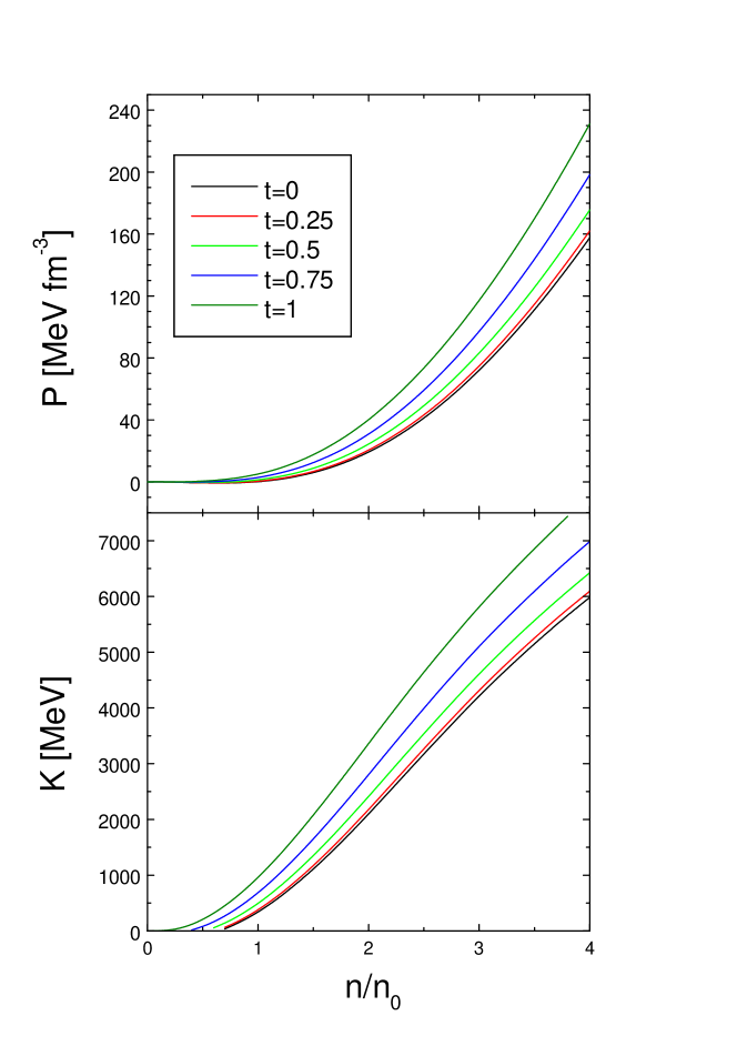
Figure 1: The pressure of cold asymmetric nuclear matter versus density for the CC case (upper panel). The different lines correspond to some typical values of the asymmetry parameter $t$. In the lower panel the corresponding compressibility $\kappa$ is shown for the same set of $t$ values.

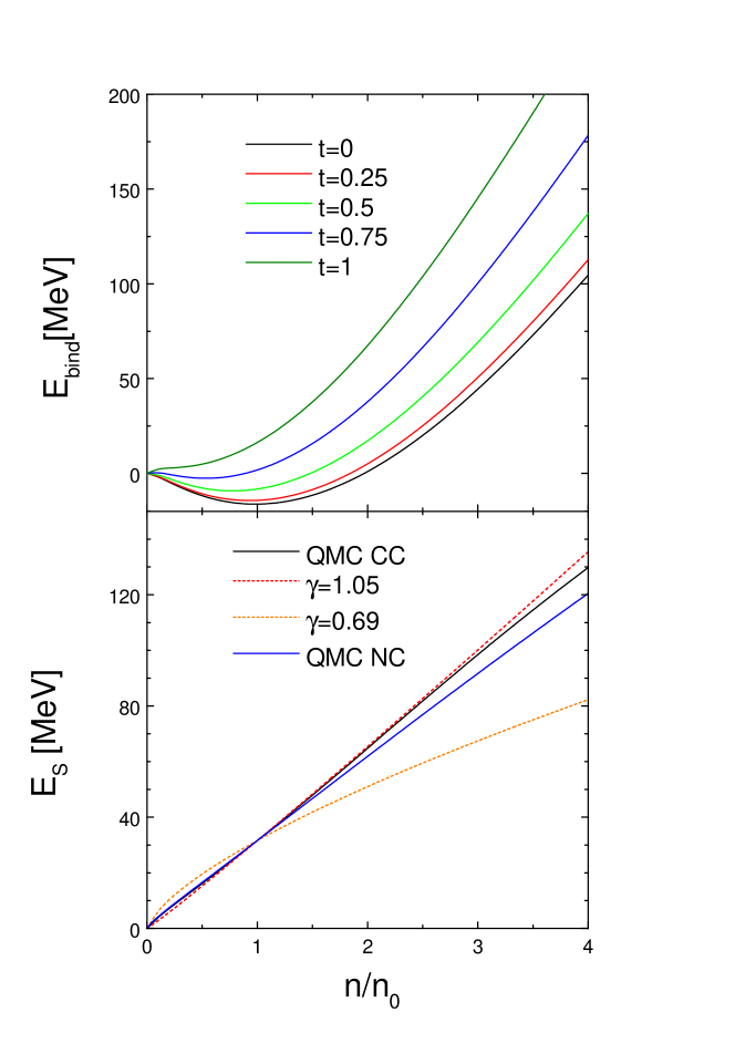
Figure 2: In the upper panel the binding energy of cold asymmetric nuclear matter for the CC case and for some typical values of the asymmetry parameter $t$ is drawn. In the lower panel we plot the asymmetry energy for the CC and NC cases, together with the empirical expression $E_{s}=31.6\,(n/n_{0})^{\gamma}$ ($\gamma=0.69,1.05$) Ref.[2].

where $M=938.92\mbox{MeV}/{c^{2}}$ is the average free nucleon rest mass.
The constraint of the symmetry energy alone is not sufficient to determine unambiguously both $g_{\rho}$ and $g_{\delta}$, instead it establishes a non-linear relation between them. In order to restrain their possible variation, we have used valuable phenomenological data coming from the analysis of isospin diffusion in heavy ion collisions [3], as discussed below.
The values of the couplings are sensitive to either the inclusion or not of the excluded volume corrections. Both instances are considered in Table 1.
The cases with the excluded volume correction (CC) have been compared with calculations without it (NC). It must be emphasized that in the last case the values $\xi=\vartheta=1$, and $\Delta\mu^{p}=\Delta\mu^{n}=0$ must be used.
With this set of parameters the equation of state for asymmetric nuclear matter with finite nucleon size has been evaluated. The results are displayed in Fig. 1 for the the pressure $P$ and the nuclear compressibility $\kappa$ in terms of the baryonic number density for several isospin asymmetries. For symmetric nuclear matter ($t=0$) at normal density we obtained $\kappa=340MeV$, which is higher than the usually assumed values in similar calculations. However it should be stressed that recent mass measurements of the pulsar PSR J0751+18007 yield $M=2.1\pm 0.2M_{\odot}$ [19], which is hardly compatible with the usually adopted value $\kappa\approx 250$ MeV. Indeed a stiffer equation of state is needed to reach this observational constraint.
In previous investigations [13] the authors found that finite baryonic size are responsible for a $12\%$ increment in the maximum mass of a neutron star, obtaining $M_{max}=1.89M_{\odot}$. Therefore the strong baryonic repulsion previous to the Quark-Gluon Plasma transition contributes significatively to produce a stiffer equation of state, and consequently it would give a phenomenological basis to understand the unexpectedly high value measured for the PSR J0751+18007 mass.
The compressibility becomes negative at low densities leading to thermodynamical instabilities, but it grows with increasing $t$ at a fixed density. The instabilities disappear for nuclear compositions approaching pure neutron matter ($t=1$) as a consequence of the repulsive character of the asymmetry energy.
The effect of increasing asymmetry on the binding energy $E_{bind}$ can be appreciated in the upper panel of Fig. 2. In particular neutron matter remains unbound for all densities. A comparison of the equation of state for the CC and NC cases was given in [13] for hadronic matter in $\beta$-equilibrium, the conclusions given there can be extended to the case of nuclear matter at fixed isospin asymmetry, i. e. density dependence for energy and pressure are stiffer in the CC instance.
In the lower panel of the same figure the asymmetry energy $E_{s}$ is displayed, together with the curves corresponding to the empirical expression $E_{s}=31.6\,(n/n_{0})^{\gamma}$ evaluated at the limit values $\gamma=0.69$ and $\gamma=1.05$ obtained in Ref.[2]. It can be seen that our result lies between these curves, showing a significative agreement with the $\gamma=1.05$ case in all the range $0.5<n/n_{0}<2.5$. It must be mentioned that within this model, only a narrow range of values for the pair of couplings $g_{\delta},g_{\rho}$ is able to fit the reference value for $E_{s}(n_{0})$ and to produce simultaneously a curve entirely comprised between the phenomenological constraints. For very low values of $g_{\rho}$ it is not possible to adjust the symmetry energy at the normal density, increasing this coupling yields a stiffer density dependence for $E_{s}(n)$, which quickly goes beyond the curve $\gamma=1.05$ of Fig.2.
Assuming a decomposition

$$E_{s}(n)=E_{s}(n_{0})+L(n/n_{0}-1)/3+K_{s}(n/n_{0}-1)^{2}/18,$$

we have found $L\simeq 95.8$ MeV and $K_{s}\simeq 19$ MeV. The first quantity agrees with the value $L=88\pm 25$ MeV found in [1], whereas we obtained for the combination $K_{asy}=K_{s}-6\,L=-555\pm 5$ MeV in comparison with the suggested value $K_{asy}=-500\pm 50$ MeV [2]. It must be pointed out that the empirical value for $L$ is coherent with the inequality $0.7<\gamma<1.1$, however the numerical value extracted from experimental data for $K_{asy}$ favors a stiffer symmetry energy with $1.26<\gamma<1.3$.
A comparison between NC and CC results yields a enhanced growth for $E_{s}(n)$ in the last case, although differences become appreciable for densities higher than $2n_{0}$. For the NC case the values $L=91.4\pm 0.6$ MeV and $K_{asy}=-553\pm 2$ MeV have been obtained.
In the limit of point-like baryons the formulae for the compressibility and the symmetry energy reduce to

$$\kappa_{t=0}=9n\left[C_{\omega}+\frac{\pi^{2}}{2k_{F}E}-\frac{C_{\sigma}^{eff}}{1+C_{\sigma}^{eff}H^{(2)}}\left(\frac{M}{E}\right)^{2}\right],$$

$$E_{s}=\frac{n}{2}\left[C_{\rho}+\frac{\pi^{2}}{2k_{F}E}-\frac{C_{\delta}^{eff}}{1+C_{\delta}^{eff}H^{(2)}}\left(\frac{M}{E}\right)^{2}\right],$$

which agree with results obtained in relativistic field models with structureless nucleons, with exception of the couplings $C_{\phi}^{eff}=\left(g_{\phi}Q/m_{\phi}\right)^{2}$ ($\phi=\sigma,\delta$) which includes the factor $Q$ defined below Eq. (3.6). Taking into account that $Q$ depends on the medium properties through $m^{\ast}_{q}$ and $R$, density dependent effective couplings have been obtained, due to the quark structure of nucleons proposed in the model.

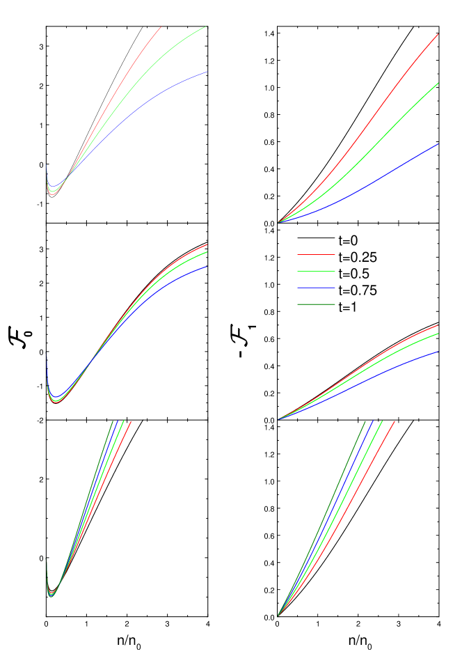
Figure 3: The adimensional Landau parameters for the CC case. In the left (right) panels the scalar (vector) components for the $p\,p$, $p\,n$, and $n\,n$ pairs are respectively plotted from top to bottom, at several fixed values of $t$. The line convention valid for all the cases is indicated in the central right panel, it must be noted that $t=1$ is relevant only for the $n\,n$ amplitude.

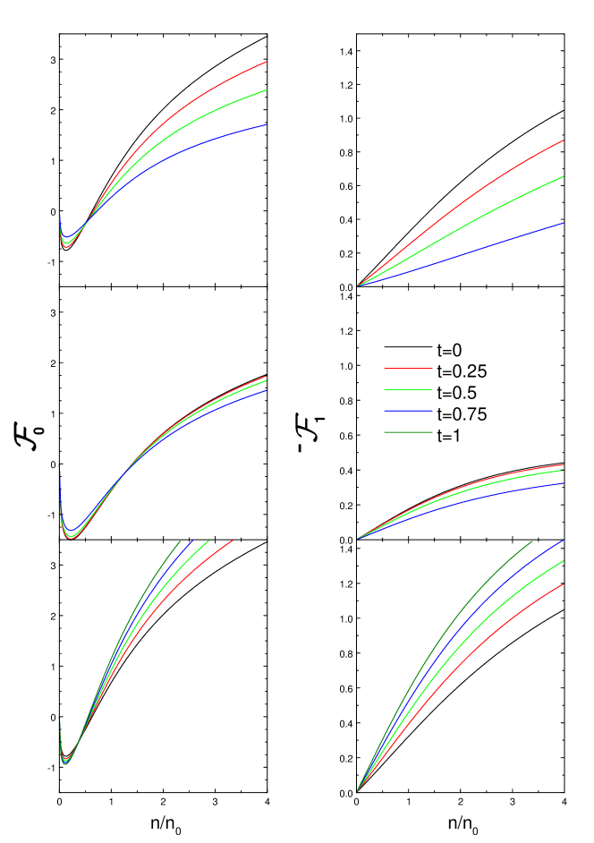
Figure 4: Idem as Fig.3, but for the NC case.

The density dependence of the adimensional Landau parameters are plotted in Figs. 3 (CC) and 4 (NC). At sufficient low densities all scalar parameters $\mathcal{F}_{p\,p}^{0}$, $\mathcal{F}_{n\,p}^{0}$, and $\mathcal{F}_{n\,n}^{0}$ are negative, reflecting the attractive character of the effective nucleon interaction. Therefore instabilities in the equation of state can appear in this density range. Comparing Figs. 3 and 4 we appreciate that, for densities $n/n_{0}\lesssim 1$, the general trend of excluded volume correlations is to slightly increase the nucleon-nucleon attraction. On the other hand in the range $n/n_{0}>1$ the volume corrections enhance the repulsion among nucleons as compared with the respective NC cases. This fact is expected since the available volume per nucleon decreases, resulting in a non negligible compression of the bags at higher densities [13].
The finite volume effects are more evident for the $\mathcal{F}_{b\,b^{\prime}}^{1}$ ($b,b^{\prime}=p,n$) components, enhancing their absolute values for all the range of densities, specially for $n/n_{0}>1$.
Because the adimensional Landau parameters contain density dependent factors, $\mathcal{F}_{p\,p}^{0,\,1}$ and $\mathcal{F}_{p\,n}^{0,\,1}$ decrease for growing isospin asymmetry $t$ as they are a measure of the strength of the in-medium proton interaction. The opposite is true for $\mathcal{F}_{n\,n}^{0,\,1}$.
The low density limit of CC results qualitatively agree with others calculations [15, 16], both for nuclear symmetric matter and for the pure neutron case.
It can be seen that in the sub-nuclear realm of the scalar interaction, the in-medium $p-n$ strength overrides the $p-p$ and $n-n$ components. Furthermore the $n-p$ attractive effect has a wider density range, extending beyond the normal value $n_{0}$.

Collective quantum fluctuations give rise to proper modes which are solutions of the eigenvalue equation (4.15). The corresponding dispersion relations $(\omega/q)$ are displayed in Figs. 5 (CC) and 6 (NC), for some typical values of the isospin asymmetry $t$. It must be pointed out that stable modes satisfy $s_{p,n}>1$, whereas pure imaginary values correspond to unstable propagation. In the last case the quantity $|\omega/q|$ has been plotted. With exception of nearly pure neutron matter, unstable modes are always present at very low densities and therefore they are practically insensitive to finite volume effects.

As it was mentioned earlier, collective modes can be classified as isoscalar and isovector, according to proton and neutron vibrations being in phase or in opposition, respectively.
Unstable modes are found to be isoscalar in character, reflecting the fact that both isospin components simultaneously undergo a liquid-vapor phase transition, leading to cluster formation [18]. This associated mechanical instability is evidenced by the negative sign of the nuclear compressibility in this density domain. Since $\kappa$ comprises density variations at fixed isospin asymmetry $t$, Eq.(3.8), it preserves the proton to neutron ratio.
It is easily verified that for the symmetric case isoscalar modes (stable or unstable) also conserve this ratio, namely $\varrho$ equals ${(\delta n^{p}/\delta n^{n})}_{t}=(n^{p}/n^{n})$ for $t=0$. This is no longer true for iso-asymmetric matter.
For growing asymmetry $t$ these unstable modes show a decreasing amplitude, because the repulsive n-n interaction progressively dominates, until the instability vanishes.
For stable eigensolutions $(\omega/q)$ represents the zero sound velocity $V_{s}$. In the iso-symmetric case there are two stable modes, both in CC and NC instances. The isovector branch appears at very low densities, whereas the isoscalar one starts at $n/n_{0}>1$ . For the CC plot they cross each other at $n/n_{0}\simeq 1.51$ ($n/n_{0}\simeq 1.9$ for NC), but keep their own character because isoscalar and mechanical oscillations preserve the same proton to neutron ratio for $t=0$. Thus, they do not couple to isovector fluctuations, which are related to species separation [18].
In general for iso-asymmetric matter there is only one stable branch which has a mixed character. In fact, the ratio of proton to neutron amplitudes $\varrho$ changes smoothly from negative (isovector) to positive (isoscalar) as the density increases. When the nucleon finite size is considered (CC) the change of character takes place at lower densities than in the point-like case (NC), as can be appreciated from figures 5 and 6, respectively.
As mentioned before, in asymmetric matter the ratio $\varrho$ for isoscalar modes (either stable or not) do not follow the constraint of keeping $t$ constant, as mechanical oscillations do [18]. In fact, the asymmetry of the medium induces a more complicated scenario where some chemical component is also involved, i.e. the relative proton to neutron concentration is modified along the quantum mode. The mixed iso-character of the stable modes at finite $t$ can be ascribed to this cause. At low densities these collective modes are isovector like, indicating a significative species separation. As the density grows, pressure (mechanical) effects become dominant and induce the change to isoscalar like character.
For pure neutron matter only one stable mode has been found in this range of densities.
Concerning the velocity of propagation, a rough $30\%$ increment in the CC results for $V_{s}$ are observed in the high density domain as compared to the NC ones. As an artifact of the approximation used to solve the Landau’s kinetic equation, it is found that $V_{s}$ approaches the velocity of light at densities $n/n_{0}\gtrsim 4$, in the CC approach. However, for such high densities the dissipative effects are non-negligible, resulting in a more involved dynamics which is beyond the scope of the present work.

6 Conclusions

We have studied the thermodynamical properties and collective modes of cold asymmetric nuclear matter. This has been performed within a model of structured nucleons, taking into account an appropriate normalization of the nucleon fields to prevent overlapping of the quark confining regions at high densities [13]. Many body properties of hadronic matter are interpreted in a Fermi liquid picture with quasiparticles and collective modes.
Within this framework the relativistic Landau parameters for iso-asymmetric nuclear matter have been evaluated, and an explicit relation with the nuclear compressibility $\kappa$ and symmetry energy $E_{s}$ has been obtained. The overall trend of excluded volume correlations at densities $n>n_{0}$ is to develop an stiffer equation of state, relative to the case where they are absent.
Different quantities such as density dependence of the symmetry energy, its slope, and the asymmetry compressibility $K_{assy}$ have been evaluated, obtaining qualitative agreement with empirical estimates.
It is argued that short range hadronic correlations in the dense medium preceding the deconfinement phase transition, which has been parametrized in the present work as excluded volume corrections, contribute to understand the high neutron star mass measured recently.
We have also applied the present formalism to the Landau’s collisionless kinetic equation for small fluctuations around the Fermi level. We have obtained the eigenvalue equation for instability and zero sound modes within this scheme, and have discussed the propagation of these modes in the dense hadronic medium.
The behavior of collective excitations can have important consequences in heavy ion reactions, where the formation of fragments is chiefly governed by isoscalar fluctuations.

Case	$g_{\sigma}^{u,d}$	$g_{\omega}^{u,d}$	$g_{\delta}^{u,d}$	$g_{\rho}^{u,d}$
CC	5.76314	2.78280	5.75150	4.3500
NC	5.99339	3.00770	5.42075	4.5000

Table 1: The quark-meson couplings used in the case with excluded volume correction (CC) and without it (NC).

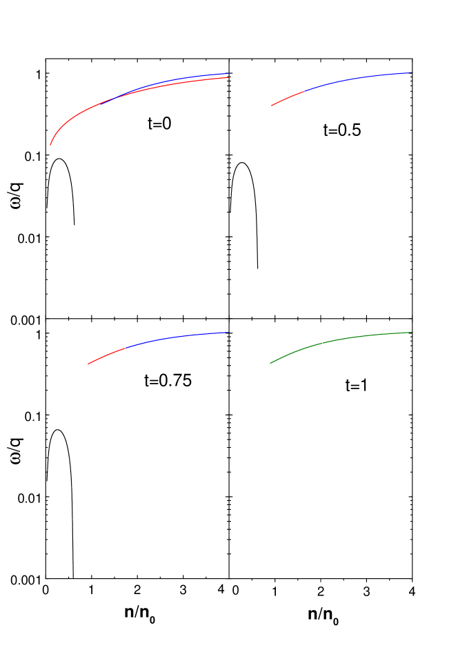
Figure 5: Dispersion relation for collective modes in the CC case, for several values of the asymmetry parameter $t$. The low density solution represents the unstable isoscalar mode (black line). The remaining stable modes are depicted with red or blue lines for isovector or isoscalar character, respectively.

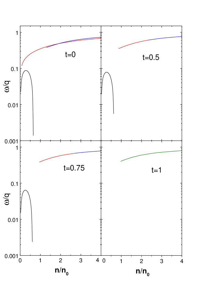
Figure 6: Idem as Fig.5, but for the NC case.

References

• [1] B.A. Li, Phys. Rev. Lett. 88 (2002) 192701;
L.W. Chen, C.M. Ko, and B.A. Li, Phys. Rev. Lett. 94 (2005) 032701, Phys. Rev C 72 (2005) 064309.
• [2] B.A. Li and L.W. Chen, Phys. Rev. C 72 (2005) 064611.
• [3] A.W. Steiner, M. Prakash, J.M. Lattimer, and P.J. Ellis, Phys. Rep. 411 (2005) 325.
• [4] D.V. Shetty, S.J. Yennello, and G.A. Souliotis, LANL Report nucl-ex/0505011.
• [5] S.S. Avancini, L. Brito, D.P. Menezes, and C. ProvidΓͺncia, Phys. Rev. C 71 (2005) 044323.
• [6] B. D. Serot and J. D. Walecka, Advan. Nucl. Phys 16, 1 (1986); Int. J. Mod. Phys. E 6, 515 (1997).
• [7] B. Liu, V. Greco, V. Baran, M. Colonna, and M. Di Toro, Phys. Rev. C65 (2002) 045201;
A. Sulaksono, P. T. P. Hutauruk, and T. Mart, Phys. Rev. C72 (2005) 065801.
• [8] P. A. M. Guichon, Phys. Lett. B200, 235 (1988);
K. Saito and A. W. Thomas, Phys. Lett. B327, 9 (1994); Phys. Rev. C 51, 2757 (1995).
• [9] J. Kapusta, Phys. Rev. D 23, 2444 (1981).
• [10] S. Kagiyama, A. Nakamura, T. Omodaka, Z. Phys. C 53, 163 (1992); 56, 557 (1992);
S. Kagiyama, A. Minaka, A. Nakamura, Prog. Theor. Phys. 89, 1227 (1993);
D. H. Rischke, M. I. Gorenstein, H. StΓΆcker and W. Greiner, Z. Phys. C 51, 485 (1991);
C. P. Singh, B. K. Patra, K. K. Singh, Phys. Lett. B387, 680 (1996);
• [11] J. Cleymans and H. Satz, Z. Phys. C 57, 135 (1993);
J. Cleymans , M. I. Gorenstein, J. StΓ₯lnacke, E. Suhonen, Phys. Scripta 48, 277 (1993);
H. Kouno, K. Koide, T. Mitsumori, N. Noda, A. Hasegawa, M. Nakano, Prog. Theor. Phys. 96, 191 (1996);
G. D. Yen, M. I. Gorenstein, W. Greiner, S. N. Yang, Phys. Rev. C 56, 2210 (1997);
M. I. Gorenstein, H. StΓΆcker, G. D. Yen, S. N. Yang, W. Greiner, J. Phys. G 24, 1777 (1998).
• [12] R. Aguirre and A.L. De Paoli, LANL Report nucl-th/9907087,
P.K. Panda, M. Bracco, M. Chiapparini, E. Conte and G. Krein, Phys. Rev. C 65 (2002) 065206
H. Miao, G. Chong Shou, and P. Zhuang, LANL Report hep-ph/0511245
• [13] R. Aguirre and A.L. De Paoli, Phys. Rev. C 68 (2003) 055804.
• [14] Landau Fermi-Liquid Theory, G. Baym and C. Phethick, John Wiley & Sons, Inc. (1991).
• [15] T. Matsui, Nucl. Phys. A 370 (1981) 365.
• [16] J.C. Caillon, P. Gabinski and J. Labarsouque, J. Phys. G 29 (2003) 2291.
• [17] K. Saito, K. Tsushima and A. W. Thomas, LANL Report nucl-th/9901084.
• [18] V. Baran, M. Colonna, V. Greco, M. Di Toro, Phys. Rep. 410 (2005) 335.
• [19] D.J. Nice et al., Astrop. J. 634 (2005)1242.