$\Lambda\alpha$, $\Sigma\alpha$ and $\Xi\alpha$ potentials derived from the $SU_{6}$ quark-model baryon-baryon interaction

Abstract

We calculate $\Lambda\alpha$, $\Sigma\alpha$ and $\Xi\alpha$ potentials from the nuclear-matter $G$-matrices of the $SU_{6}$ quark-model baryon-baryon interaction. The $\alpha$-cluster wave function is assumed to be a simple harmonic-oscillator shell-model wave function. A new method is proposed to derive the direct and knock-on terms of the interaction Born kernel from the hyperon-nucleon $G$-matrices, with explicit treatments of the nonlocality and the center-of-mass motion between the hyperon and $\alpha$. We find that the $SU_{6}$ quark-model baryon-baryon interactions, FSS and fss2, yield a reasonable bound-state energy for ${}^{5}_{\Lambda}\hbox{He}$, $-3.18\sim-3.62$ MeV, in spite of the fact that they give relatively large depths for the $\Lambda$ single-particle potentials, 46 $\sim$ 48 MeV, in symmetric nuclear matter. An equivalent local potential derived from the Wigner transform of the nonlocal $\Lambda\alpha$ kernel shows a strong energy dependence for the incident $\Lambda$-particle, indicating the importance of the strangeness-exchange process in the original hyperon-nucleon interaction. For the $\Sigma\alpha$ and $\Xi\alpha$ potentials, we only discuss the zero-momentum Wigner transform of the interaction kernels, since these interactions turn out to be repulsive when the two isospin contributions for the $\Sigma N$ and $\Xi N$ interactions are added up. These components show a strong isospin dependence: They are attractive in the isospin $I=1/2$ ($\Sigma\alpha$) and $I=0$ ($\Xi\alpha$) components and repulsive in $I=3/2$ ($\Sigma\alpha$) and $I=1$ ($\Xi\alpha$) components, which indicate that $\Sigma$ and $\Xi$ potentials could be attractive in some particular systems such as the well-known ${}^{4}_{\Sigma}\hbox{He}$ system.

1 Introduction

Interactions between the octet baryons ($B_{8}=N,~{}\Lambda,~{}\Sigma$ and $\Xi$) and the $\alpha$ cluster are important ingredients to consider the possible existence for various kinds of light hypernuclei through detailed microscopic cluster-model calculations. If reliable effective $B_{8}N$ interactions were known, one could easily calculate the $B_{8}\alpha$ potentials, using the standard cluster-model techniques. Unfortunately, this is not the case except for $B_{8}=N$, since the bare $B_{8}N$ interaction itself is not well known especially for the $\Sigma$ and $\Xi$ hyperons, because of the technical difficulties of strangeness experiments. Even if these bare interactions were eventually known, we further need to develop the procedure to link the bare interactions and effective interactions through some effective interaction theory such as the $G$-matrix formalism.

We have recently developed the QCD-inspired spin-flavor $SU_{6}$ quark model for the baryon-baryon interaction [1], which is a unified model for the full octet-baryons [2], and have achieved accurate descriptions of the $NN$ and $YN$ interactions [3]. In particular, the $NN$ interaction of the most recent model fss2 is accurate enough to compare with modern realistic meson-exchange models. These quark-model interactions were used for the detailed study of few-baryon systems such as ${}^{3}\hbox{H}$ [4, 5] and ${}^{3}_{\Lambda}\hbox{H}$ [6], and also of some typical $\Lambda$-hypernuclei, ${}^{9}_{\Lambda}\hbox{Be}$ [7, 8] and ${}^{\ \,6}_{\Lambda\Lambda}\hbox{He}$ [9], through a newly developed three-cluster Faddeev formalism [10, 11] and $G$-matrix calculations [12, 13, 14]. We can now use these baryon-baryon interactions to calculate not only the $\Lambda\alpha$ interaction, but also $\Sigma\alpha$ and $\Xi\alpha$ interactions, assuming the harmonic-oscillator (h.o.) shell-model wave function for the $\alpha$-cluster.

There are, in fact, a couple of advanced procedure to derive the interactions between a single baryon and finite nuclei based on the density-dependent Hartree-Fock theory of $G$-matrix interactions [15, 16, 17]. These approaches, however, use the localized $G$-matrix interaction in the configuration space and the center-of-mass (c.m.) coordinate system connected to the target nucleus. For the $B_{8}\alpha$ interactions, the c.m. correction is quite important. In this paper, we will derive $B_{8}\alpha$ Born kernels, directly starting from the $G$-matrix calculation of the quark-model baryon-baryon interactions. We deal with the nonlocality of the $G$-matrix and the c.m. motion exactly, using the cluster-model approach, at the expense of the self-consistency between the $\alpha$-cluster formation and the $G$-matrix interaction. The $G$-matrix is pre-determined by solving the Bethe-Goldstone equation in symmetric nuclear matter, and the momentum-dependent single-particle (s.p.) potentials as well [12]. The Fermi-momentum is assumed to be the standard value $k_{F}=1.35~{}\hbox{fm}^{-1}$, but the obtained $B_{8}\alpha$ interactions depend on this choice rather monotonously, except for some special cases such as the $\Lambda\alpha$ $LS$ interaction. The treatment of the starting-energy dependence and the non-Galilean invariant momentum dependence of the $G$-matrix is explicitly discussed. We believe that these approximations are good enough to understand the unknown $\Sigma\alpha$ and $\Xi\alpha$ interactions qualitatively, starting from the quark-model predictions of various baryon-baryon interactions. For the $\Lambda\alpha$ interaction, we compare the predictions by the present approach with some available phenomenological $\Lambda\alpha$ potentials [7, 18], obtained by various methods. Another application of the present approach to the $N\alpha$ interaction will be published in a separate paper, since this system involves an extra nucleon-exchange term.

Since the obtained $B_{8}\alpha$ interactions are all nonlocal, we calculate the Wigner transform from the $B_{8}\alpha$ Born kernels. We find that the momentum dependence of the Wigner transform is very strong, and the procedure to find effective local potential by solving the transcendental equation is necessary to obtain a local-potential image for the $\Lambda\alpha$ interaction. The $\Sigma\alpha$ and $\Xi\alpha$ interactions are repulsive, although the isospin $I=1/2$ (for $\Sigma\alpha$) and $I=0$ (for $\Xi\alpha$) contributions of the $\Sigma N$ and $\Xi N$ interactions are attractive. As the first step to study realistic $\Sigma\alpha$ and $\Xi\alpha$ interactions, we will only discuss the zero-momentum Wigner transform in this paper. Although these $B_{8}\alpha$ interactions are complex due to the imaginary part of the underlying $G$-matrices, we discuss only the real part. The spin-orbit $B_{8}\alpha$ potentials are naturally obtained from the $LS$ and $LS^{(-)}$ components of the $G$-matrix invariant interaction.

The central $\Lambda\alpha$, $\Sigma\alpha$ and $\Xi\alpha$ potentials were calculated by many authors with other (usually more crude or purely phenomenological) approaches. The $\Lambda\alpha$ potential was calculated numerously, and different shapes were considered. For instance, see Refs. [19, 20, 21, 22]. Some phenomenological $\Sigma\alpha$ and $\Xi\alpha$ potentials are found in Ref. [23, 24, 25, 26]. The comparison of our results with these potentials are, however, not easy, since our Wigner transform is momentum-dependent and the solutions of the transcendental equations are strongly energy-dependent. We will only point out if some resemblance between them are found. The importance of the isospin dependence of the $\Sigma N$ and $\Xi N$ interactions to the $\Sigma$-nucleus and $\Xi$-nucleus potentials has been discussed by many authors from the phenomenological aspects, for example, in Refs. [27, 23, 25], and by Rijken and Yamamoto from the viewpoint of $G$-matrix calculations in Ref. [28].

The organization of this paper is as follows. In the next formulation section, we first give in Section 2.1 the basic folding formula for the $\alpha$-cluster based on the separation of the $B_{8}\alpha$ Born kernel to the spin-isospin factors and the spatial part. The treatment of $G$-matrix variables, the starting energy and the c.m. momentum, will be carefully discussed. A convenient transformation formula for the rearrangement of relative momenta is given in Section 2.2, by which the partial wave component of the $B_{8}\alpha$ Born kernel is explicitly given both for the central component and the $LS$ component. The folding formula in the partial-wave expansion and the partial-wave components of the $B_{8}\alpha$ Born kernel are explicitly given in Section 2.3. A procedure to calculate the Wigner transform is given in Section 2.4 with a couple of approximations. One of the approximations for the $LS$ component yields a simple factor for the strength of the $LS$ potential, which corresponds to the well-known Scheerbaum factor $S_{B}$ [29] in nuclear matter. The Section 3 is devoted to the results and discussion; first in Section 3.1 the $\Lambda\alpha$ central and $LS$ potentials both in the $T$-matrix approach and in the Wigner transform approach. The isospin dependence of the $\Sigma\alpha$ and $\Xi\alpha$ potentials is discussed in Section 3.2. Section 4 is devoted to a summary. The invariant $G$-matrix for the most general $B_{8}B_{8}$ interaction is discussed in Appendix A.

2 Formulation

2.1 $\alpha$-cluster folding for the $G$-matrix invariant interaction

The $B_{8}\alpha$ Born kernel for the $(0s)$ h.o. $\alpha$-cluster wave function is calculated from

$$V(\mbox{\boldmath$q$}_{f},\mbox{\boldmath$q$}_{i})=\langle\,\delta(\mbox{\boldmath$X$}_{G})e^{i\mbox{\boldmath$q$}_{f}\cdot\mbox{\boldmath$r$}}\chi_{B}\phi_{\alpha}\,|\,\sum^{5}_{j=2}G_{1j}\,|\,1\cdot e^{i\mbox{\boldmath$q$}_{i}\cdot\mbox{\boldmath$r$}}\chi_{B}\phi_{\alpha}\,\rangle\ \ ,$$ (2.1)

where $\chi_{B}$ is the spin-isospin wave function of $B$, $\phi_{\alpha}$ the internal wave function of $\alpha$, and $G_{1j}$ the $BN$ $G$-matrix acting on the particle $i=1$ ($B$) and $j=2$ - 5 (nucleons). We use the short-hand notation $B$ to specify one of the octet baryons, $B_{8}=N,~{}\Lambda,~{}\Sigma$ or $\Xi$. In Eq. (2.1), it is important to calculate the Born kernel in the total c.m. system by inserting $\delta(\mbox{\boldmath$X$}_{G})$ and 1 in the bra and ket sides, respectively [30], since the $G$-matrix interaction $G_{1j}$ is non-Galilean invariant. Namely, the two-particle $G$-matrix which satisfies the translational invariance is parametrized by

$$\langle\mbox{\boldmath$p$}_{1},\mbox{\boldmath$p$}_{2}|G|\mbox{\boldmath$p$}^{\prime}_{1},\mbox{\boldmath$p$}^{\prime}_{2}\rangle=\delta(\mbox{\boldmath$K$}-\mbox{\boldmath$K$}^{\prime})\frac{1}{(2\pi)^{3}}G(\mbox{\boldmath$p$},\mbox{\boldmath$p$}^{\prime};K,\omega,k_{F})\ \ .$$ (2.2)

Here, $\omega$ is the starting energy, $K=|\mbox{\boldmath$K$}|$ is the magnitude of the c.m. momentum, $k_{F}$ is the Fermi momentum of nuclear matter, and the relative momentum $p$ (and also $\mbox{\boldmath$p$}^{\prime}$ etc. with primes), is given by

$$p = \frac{\xi\mbox{\boldmath$p$}_{1}-\mbox{\boldmath$p$}_{2}}{1+\xi}\ \ ,\qquad\qquad\mbox{\boldmath$p$}_{1}=\frac{1}{1+\xi}\mbox{\boldmath$K$}+\mbox{\boldmath$p$}\ \ ,$$

$$K = \mbox{\boldmath$p$}_{1}+\mbox{\boldmath$p$}_{2}\ \ ,\qquad\qquad\mbox{\boldmath$p$}_{2}=\frac{\xi}{1+\xi}\mbox{\boldmath$K$}-\mbox{\boldmath$p$}\ \ ,$$ (2.3)

with $\xi=(M_{N}/M_{B})\leq 1$ being the mass ratio between the nucleon and the baryon $B$. We assume a constant $k_{F}=1.35~{}\hbox{fm}^{-1}$ in this paper unless otherwise specified, so that we will omit this index in the following. In fact, the $G$-matrix in Eq. (2.1) contains the exchange term. It is, therefore, convenient to use the isospin sum of the invariant $G$-matrix, $G^{I}_{BB}(\mbox{\boldmath$p$},\mbox{\boldmath$p$}^{\prime};K,\omega)$ with $I=I_{B}+1/2$ and $I_{B}-1/2$ ($I_{B}$ is the isospin of $B$), defined through

$$G^{I}_{BB}(\mbox{\boldmath$p$},\mbox{\boldmath$p$}^{\prime};K,\omega)$$

$$=\langle\,[BN]_{II_{z}}\,|\,G(\mbox{\boldmath$p$},\mbox{\boldmath$p$}^{\prime};K,\omega)-G(\mbox{\boldmath$p$},-\mbox{\boldmath$p$}^{\prime};K,\omega)\,P_{\sigma}\,P_{F}\,|\,[BN]_{II_{z}}\,\rangle\ \$$

$$=\left(1+\delta_{B,N}\right)\left[g^{I}_{0}+g^{I}_{ss}(\mbox{\boldmath$\sigma$}_{1}\cdot\mbox{\boldmath$\sigma$}_{2})+h^{I}_{0}\,i\widehat{\mbox{\boldmath$n$}}\cdot(\mbox{\boldmath$\sigma$}_{1}+\mbox{\boldmath$\sigma$}_{2})+h^{I}_{-}\,i\widehat{\mbox{\boldmath$n$}}\cdot(\mbox{\boldmath$\sigma$}_{1}-\mbox{\boldmath$\sigma$}_{2})\right.$$

$$\hskip 82.51299pt\left.+\cdots\right]$$ (2.4)

Here $\widehat{\mbox{\boldmath$n$}}=[\mbox{\boldmath$p$}^{\prime}\times\mbox{\boldmath$p$}]/(p^{\prime}p\sin\theta)$, and the invariant functions $g^{I}_{0}$ (central), $g^{I}_{ss}$ (spin-spin), $h^{I}_{0}$ ($LS$), $h^{I}_{-}$ ($LS^{(-)}$), etc. are functions of $\mbox{\boldmath$p$}^{2}$, ${\mbox{\boldmath$p$}^{\prime}}^{2}$, $\cos\theta=(\widehat{\mbox{\boldmath$p$}}\cdot\widehat{\mbox{\boldmath$p$}}^{\prime})$, $K$, $\omega$, and $k_{F}$. These are expressed by the partial-wave components of the $BN$ $G$-matrix as (see Appendix D of Ref. [31])

$$\left.\begin{array}[]{c}g^{I}_{0}\\ g^{I}_{ss}\\ \end{array}\right\} = \frac{1}{4}\,\sum_{J\ell S}(2J+1)\left\{\begin{array}[]{c}1\\ \frac{1}{3}[2S(S+1)-3]\end{array}\right\}G^{IJ}_{S\ell,S\ell}~{}P_{l}(\cos\theta)\ \ ,$$ (2.9)

$$h^{I}_{0} = -\frac{1}{4}\sum_{J}\frac{(2J+1)}{J(J+1)}\left[G^{IJ}_{1J,1J}~{}P^{1}_{J}(\cos\theta)\right.$$

$$\left.+J~{}G^{IJ}_{1J+1,1J+1}~{}P^{1}_{J+1}(\cos\theta)-(J+1)G^{IJ}_{1J-1,1J-1}~{}P^{1}_{J-1}(\cos\theta)\right]\ \ ,$$

$$h^{I}_{-} = \frac{1}{4}\sum_{J}\frac{(2J+1)}{\sqrt{J(J+1)}}\left[G^{IJ}_{1J,0J}+G^{IJ}_{0J,1J}\right]~{}P^{1}_{J}(\cos\theta)\ \ ,$$ (2.10)

where the argument $p$, $\mbox{\boldmath$p$}^{\prime}$, $K$, $\omega$, $k_{F}$ and subscripts for the baryon channels are omitted for the typographical reason. In the $LS$ term, $P^{1}_{J}(\cos\theta)=(\sin\theta)P^{\prime}_{J}(\cos\theta)$ with $J\geq 1$ is the associated Legendre function of the first rank. The invariant $G$-matrix for the most general $B_{8}B_{8}$ interaction is discussed in Appendix A.

In order to calculate the spin-isospin factors, it is convenient to introduce an isospin $pseudo$-exchange operator of the $BN$ system by

$$P_{\tau}=\frac{1}{2I_{B}+1}\left(1+\mbox{\boldmath$\tau$}_{B}\cdot\mbox{\boldmath$\tau$}_{N}\right)\ \ ,$$ (2.11)

with the isospin matrix elements

$$\left(\mbox{\boldmath$\tau$}_{B}\cdot\mbox{\boldmath$\tau$}_{N}\right)=\left\{\begin{array}[]{l}2I_{B}\\ -2(I_{B}+1)\\ \end{array}\right.\qquad\hbox{for}\qquad I=\left\{\begin{array}[]{l}I_{B}+1/2\\ I_{B}-1/2\\ \end{array}\right.\ \ ,$$ (2.12)

and write the invariant $G$-matrix as

$$G(\mbox{\boldmath$p$},\mbox{\boldmath$p$}^{\prime};K,\omega)=G^{I=I_{B}+1/2}_{BB}(\mbox{\boldmath$p$},\mbox{\boldmath$p$}^{\prime};K,\omega)\frac{1+P_{\tau}}{2}+G^{I=I_{B}-1/2}_{BB}(\mbox{\boldmath$p$},\mbox{\boldmath$p$}^{\prime};K,\omega)\frac{1-P_{\tau}}{2}\ \ .$$ (2.13)

We need to calculate

$$X^{I\Omega}_{B}=\langle\chi_{B}\chi_{\alpha}|\sum^{5}_{j=2}\omega^{\Omega}_{1,j}\left(\frac{1\pm P_{\tau}}{2}\right)_{1,j}|\chi_{B}\chi_{\alpha}\rangle\ \ ,$$ (2.14)

with the spin factors $\omega^{central}_{12}=1$, $\omega^{ss}_{12}=(\mbox{\boldmath$\sigma$}_{1}\cdot\mbox{\boldmath$\sigma$}_{2})$, $\omega^{LS}_{12}=\mbox{\boldmath$\sigma$}_{1}+\mbox{\boldmath$\sigma$}_{2}$, and $\omega^{LS^{(-)}}_{12}=\mbox{\boldmath$\sigma$}_{1}-\mbox{\boldmath$\sigma$}_{2}$. In Eq. (2.14), $\chi_{\alpha}$ is the spin-isospin wave function of $\alpha$; i.e., $\phi_{\alpha}=\chi_{\alpha}\phi^{\rm space}_{\alpha}$. Then we find that non-zero matrix elements are

$$X^{I\,central}_{B}=2\frac{2I+1}{2I_{B}+1}\ \ ,\qquad X^{I\,LS}_{B}=X^{I\,LS^{(-)}}_{B}=2\frac{2I+1}{2I_{B}+1}\mbox{\boldmath$\sigma$}_{1}\ \ .$$ (2.15)

On the other hand, the spatial part is calculated in Appendix (B6) of Ref. [7]. It is convenient to express this formula as

$$V^{\rm space}(\mbox{\boldmath$q$}_{f},\mbox{\boldmath$q$}_{i})=\langle\,\delta(\mbox{\boldmath$X$}_{G})e^{i\mbox{\boldmath$q$}_{f}\cdot\mbox{\boldmath$r$}}\phi^{\rm space}_{\alpha}\,|\,G^{\rm space}\,|\,1\cdot e^{i\mbox{\boldmath$q$}_{i}\cdot\mbox{\boldmath$r$}}\phi^{\rm space}_{\alpha}\,\rangle$$

$$=e^{-\frac{3}{32\nu}k^{2}}\left(\frac{2(1+\xi)^{2}}{3\pi\nu}\right)^{\frac{3}{2}}\int d\mbox{\boldmath$p$}\,\exp\left\{-\frac{2(1+\xi)^{2}}{3\nu}\left(\mbox{\boldmath$p$}-\frac{1+4\xi}{4(1+\xi)}\mbox{\boldmath$q$}\right)^{2}\right\}$$

$$\qquad\times G^{\rm space}\left(\mbox{\boldmath$p$}+\frac{1}{2}\mbox{\boldmath$k$},\mbox{\boldmath$p$}-\frac{1}{2}\mbox{\boldmath$k$};(1+\xi)|\mbox{\boldmath$q$}-\mbox{\boldmath$p$}|,\omega\right)\ \ ,$$ (2.16)

where

$$\mbox{\boldmath$k$}=\mbox{\boldmath$q$}_{f}-\mbox{\boldmath$q$}_{i}\ \ ,\qquad\mbox{\boldmath$q$}=\frac{1}{2}\left(\mbox{\boldmath$q$}_{f}+\mbox{\boldmath$q$}_{i}\right)\ \ ,$$ (2.17)

are the momentum transfer and the local momentum of the $B_{8}\alpha$ system. By assuming $g^{I}_{0}$, $h^{I}_{0}\,i\widehat{\mbox{\boldmath$n$}}$ and $h^{I}_{-}\,i\widehat{\mbox{\boldmath$n$}}$ for $G^{\rm space}$, we finally obtain

$$V(\mbox{\boldmath$q$}_{f},\mbox{\boldmath$q$}_{i})=\sum_{I\Omega}2\left(\frac{2I+1}{2I_{B}+1}\right)V^{I\Omega}(\mbox{\boldmath$q$}_{f},\mbox{\boldmath$q$}_{i})\ \ ,$$

$$V^{I\,\left({C\atop LS}\right)}(\mbox{\boldmath$q$}_{f},\mbox{\boldmath$q$}_{i})$$

$$=e^{-\frac{3}{32\nu}k^{2}}\left(\frac{2(1+\xi)^{2}}{3\pi\nu}\right)^{\frac{3}{2}}\int d\mbox{\boldmath$p$}\,\exp\left\{-\frac{2(1+\xi)^{2}}{3\nu}\left(\mbox{\boldmath$p$}-\frac{1+4\xi}{4(1+\xi)}\mbox{\boldmath$q$}\right)^{2}\right\}$$

$$\qquad\times\left\{\begin{array}[]{c}g^{I}_{0}\left(\mbox{\boldmath$p$}+\frac{1}{2}\mbox{\boldmath$k$},\mbox{\boldmath$p$}-\frac{1}{2}\mbox{\boldmath$k$};(1+\xi)|\mbox{\boldmath$q$}-\mbox{\boldmath$p$}|,\omega\right)\\ h^{I}\left(\mbox{\boldmath$p$}+\frac{1}{2}\mbox{\boldmath$k$},\mbox{\boldmath$p$}-\frac{1}{2}\mbox{\boldmath$k$};(1+\xi)|\mbox{\boldmath$q$}-\mbox{\boldmath$p$}|,\omega\right)i\widehat{[\mbox{\boldmath$p$}\times\mbox{\boldmath$k$}]}\cdot\mbox{\boldmath$\sigma$}_{1}\\ \end{array}\right\}\ \ ,$$ (2.20)

where $h^{I}=h^{I}_{0}+h^{I}_{-}$ and $\widehat{[\mbox{\boldmath$p$}\times\mbox{\boldmath$k$}]}=[\mbox{\boldmath$p$}\times\mbox{\boldmath$k$}]/|\,[\mbox{\boldmath$p$}\times\mbox{\boldmath$k$}]\,|$.

It should be noted that the c.m. momentum of the two interacting particles, $\mbox{\boldmath$K$}=(1+\xi)(\mbox{\boldmath$q$}-\mbox{\boldmath$p$})$, in Eqs. (2.16) and (2.20) implies that the local momentum $\mbox{\boldmath$q$}=(\mbox{\boldmath$q$}_{f}+\mbox{\boldmath$q$}_{i})/2$ in Eq. (2.17) plays the role of the incident momentum of the first baryon $B$ from Eq. (2.3), and $p$ the local momentum of the two-particle system, which is now an integral variable. This is a consequence of fixing the c.m. motion of the $B_{8}\alpha$ system as in Eq. (2.1), and is a special situation of the direct and knock-on (exchange) terms. The $G$-matrix depends only on the magnitude $K=|\mbox{\boldmath$K$}|$, since we make an angular average in the $G$-matrix calculation [12, 13]. The $G$-matrix value is, therefore, specified by $K$ and $\omega$, or alternatively by the incident momentum $q_{1}=|\mbox{\boldmath$q$}_{1}|$ and the relative momentum $q=|\mbox{\boldmath$q$}|$ between $B$ and $N$; i.e., $G(\mbox{\boldmath$p$},\mbox{\boldmath$p$}^{\prime};K,\omega)=G(\mbox{\boldmath$q$}+\mbox{\boldmath$k$}/2,\mbox{\boldmath$q$}-\mbox{\boldmath$k$}/2;q_{1},q)$ with $\mbox{\boldmath$k$}=\mbox{\boldmath$p$}-\mbox{\boldmath$p$}^{\prime}$ and $\mbox{\boldmath$q$}=(\mbox{\boldmath$p$}+\mbox{\boldmath$p$}^{\prime})/2$. If $q_{1}$ and $q$ are specified, $K$ is determined by the angular averaging, and $q_{2}$ is determined from $q_{1}$ and $K$. Then the starting energy $\omega$ is determined as the sum of the relative kinetic energy of two particles and the s.p. potentials for $B_{8}$ and $N$ at $q_{1}$ and $q_{2}$, respectively. We therefore choose $q_{1}=|\mbox{\boldmath$q$}_{f}+\mbox{\boldmath$q$}_{i}|/2$ and $q=|\mbox{\boldmath$p$}|$ in the $G$-matrix in Eqs. (2.16) and (2.20). In order to carry out this rather involved calculation, we will develop in the next subsection some kind of transformation formula for the rearrangement of relative momenta in the partial-wave components of nonlocal kernels.

2.2 A transformation formula of the nonlocal kernel in the momentum representation

The folding formula in Eq. (2.16) implies that expressing the $G$-matrix interaction $G^{C}(\mbox{\boldmath$p$},\mbox{\boldmath$p$}^{\prime})$ and $G^{LS}(\mbox{\boldmath$p$},\mbox{\boldmath$p$}^{\prime})\,i\widehat{[\mbox{\boldmath$p$}^{\prime}\times\mbox{\boldmath$p$}]}\cdot\mbox{\boldmath$S$}$ with the subsidiary momentum variables

$$k = \mbox{\boldmath$p$}-\mbox{\boldmath$p$}^{\prime}\ \ ,\qquad\qquad\mbox{\boldmath$p$}=\mbox{\boldmath$q$}+\frac{1}{2}\mbox{\boldmath$k$}\ \ ,$$

$$q = \frac{1}{2}(\mbox{\boldmath$p$}+\mbox{\boldmath$p$}^{\prime})\ \ ,\qquad\mbox{\boldmath$p$}^{\prime}=\mbox{\boldmath$q$}-\frac{1}{2}\mbox{\boldmath$k$}\ \ ,$$ (2.21)

is convenient for the $\alpha$-cluster folding. We express these kernels using the calligraphic letters; i.e.,

$${\mathcal{G}}^{C}(\mbox{\boldmath$k$},\mbox{\boldmath$q$})=G^{C}(\mbox{\boldmath$p$},\mbox{\boldmath$p$}^{\prime})\ \ ,$$

$${\mathcal{G}}^{LS}(\mbox{\boldmath$k$},\mbox{\boldmath$q$})\,i\widehat{[\mbox{\boldmath$q$}\times\mbox{\boldmath$k$}]}\cdot\mbox{\boldmath$S$}=G^{LS}(\mbox{\boldmath$p$},\mbox{\boldmath$p$}^{\prime})\,i\widehat{[\mbox{\boldmath$p$}^{\prime}\times\mbox{\boldmath$p$}]}\cdot\mbox{\boldmath$S$}\ \ .$$ (2.22)

By using this notation and the $q_{1}$, $q$ notation for $K$, $\omega$, discussed in the last subsection, $G^{\rm space}$ in Eq. (2.16), for example, becomes ${\mathcal{G}}^{\rm space}(\mbox{\boldmath$k$},\mbox{\boldmath$p$};q_{1},p)$ with $q_{1}=|\mbox{\boldmath$q$}_{f}+\mbox{\boldmath$q$}_{i}|/2$. In the following, we omit the argument $K$, $\omega$ or $q_{1}$, $q$ for simplicity, unless the dependence becomes crucial for the relationship under consideration. After making partial wave decomposition in Eq. (2.22), we can easily carry out the integral over $p$. The resultant expression is denoted by ${\mathcal{V}}^{C}(\mbox{\boldmath$k$},\mbox{\boldmath$q$})$ and by ${\mathcal{V}}^{LS}(\mbox{\boldmath$k$},\mbox{\boldmath$q$})\,i\widehat{[\mbox{\boldmath$q$}\times\mbox{\boldmath$k$}]}\cdot\mbox{\boldmath$S$}$. The desired Born kernels, $V^{C}(\mbox{\boldmath$q$}_{f},\mbox{\boldmath$q$}_{i})$ and $V^{LS}(\mbox{\boldmath$q$}_{f},\mbox{\boldmath$q$}_{i})\,i\widehat{[\mbox{\boldmath$q$}_{i}\times\mbox{\boldmath$q$}_{f}]}\cdot\mbox{\boldmath$S$}$, are obtained from another transformation related to Eq. (2.17).

Our task is, therefore, to relate the partial-wave components ${\mathcal{G}}^{C}_{\lambda}(k,q)$ and $G^{C}_{\ell}(p,p^{\prime})$, and also ${\mathcal{G}}^{LS}_{\lambda}(k,q)$ and $G^{LS}_{\ell}(p,p^{\prime})$, which are defined through

$${\mathcal{G}}^{C}(\mbox{\boldmath$k$},\mbox{\boldmath$q$})=\sum^{\infty}_{\lambda=0}(2\lambda+1){\mathcal{G}}^{C}_{\lambda}(k,q)P_{\lambda}(\widehat{\mbox{\boldmath$k$}}\cdot\widehat{\mbox{\boldmath$q$}})\ \ ,$$

$$G^{C}(\mbox{\boldmath$p$},\mbox{\boldmath$p$}^{\prime})=\sum^{\infty}_{\ell=0}(2\ell+1)G^{C}_{\ell}(p,p^{\prime})P_{\ell}(\widehat{\mbox{\boldmath$p$}}\cdot\widehat{\mbox{\boldmath$p$}}^{\prime})\ \ ,$$

$${\mathcal{G}}^{LS}(\mbox{\boldmath$k$},\mbox{\boldmath$q$})=\sum^{\infty}_{\lambda=1}(2\lambda+1){\mathcal{G}}^{LS}_{\lambda}(k,q)P^{1}_{\lambda}(\widehat{\mbox{\boldmath$k$}}\cdot\widehat{\mbox{\boldmath$q$}})\ \ ,$$

$$G^{LS}(\mbox{\boldmath$p$},\mbox{\boldmath$p$}^{\prime})=\sum^{\infty}_{\ell=1}(2\ell+1)G^{LS}_{\ell}(p,p^{\prime})P^{1}_{\ell}(\widehat{\mbox{\boldmath$p$}}\cdot\widehat{\mbox{\boldmath$p$}}^{\prime})\ \ .$$ (2.23)

We generalize the transformation Eq. (2.21) as

$$\left(\begin{array}[]{c}\mbox{\boldmath$p$}\\ \mbox{\boldmath$p$}^{\prime}\\ \end{array}\right)=\left(\begin{array}[]{cc}\frac{1}{2}&1\\ -\frac{1}{2}&1\\ \end{array}\right)\left(\begin{array}[]{c}\mbox{\boldmath$k$}\\ \mbox{\boldmath$q$}\\ \end{array}\right)=\left(\begin{array}[]{cc}\alpha&\beta\\ \gamma&\delta\\ \end{array}\right)\left(\begin{array}[]{c}\mbox{\boldmath$k$}\\ \mbox{\boldmath$q$}\\ \end{array}\right)\ \ ,$$ (2.34)

with $\alpha\delta-\beta\gamma=1$. A simple calculation gives

$${\mathcal{G}}^{C}_{\lambda}(k,q)=\sum^{\infty}_{\ell=0}(2\ell+1)\frac{1}{2}\int^{1}_{-1}dx~{}\frac{G^{C}_{\ell}(p,p^{\prime})}{(pp^{\prime})^{\ell}}P_{\lambda}(x)\,g_{\ell}(k,q;x)\ \ ,$$ (2.35)

where $g_{\ell}(k,q;x)=(pp^{\prime})^{\ell}P_{\ell}(\widehat{\mbox{\boldmath$p$}}\cdot\widehat{\mbox{\boldmath$p$}}^{\prime})$ with

$$p=\sqrt{\alpha^{2}k^{2}+\beta^{2}q^{2}+2\alpha\beta kqx}\ \ ,\qquad p^{\prime}=\sqrt{\gamma^{2}k^{2}+\delta^{2}q^{2}+2\gamma\delta kqx}\ \ .$$ (2.36)

The transformation of the $LS$ components is similarly carried out by using the orthogonality relations of $P^{1}_{\ell}(x)$ and

$$\left(\frac{1}{\sin\theta}\right)P^{1}_{\ell}(\cos\theta)=\sum_{\ell^{\prime}=\ell-1,\ell-3,\cdots,1~{}{\rm or}~{}0}(2\ell^{\prime}+1)\,P_{\ell^{\prime}}(\cos\theta)\ \ ,$$

$$P_{\lambda-1}(x)-P_{\lambda+1}(x)=\frac{2\lambda+1}{\lambda(\lambda+1)}\sqrt{1-x^{2}}\,P^{1}_{\lambda}(x)\ \ .$$ (2.37)

For the numerical integration over $x$ in Eq. (2.35) etc., it is convenient to use the spline interpolation

$$G^{\Omega}_{\ell}(p,p^{\prime})=\sum_{i,j}S_{i}(p)\,S_{j}(p^{\prime})\,G^{\Omega}_{\ell}(p_{i},p_{j})\ \ ,$$ (2.38)

since the G-matrix calculation itself is very much time consuming. After all, we obtain the following formula for the transformation of the partial-wave components:

$${\mathcal{G}}^{\Omega}_{\lambda}(k,q)=\sum_{i,j}\sum^{\infty}_{\ell=0~{}{\rm or}~{}1}(2\ell+1)\,F^{\Omega\,\lambda\ell}_{i,j}\,G^{\Omega}_{\ell}(p_{i},p_{j})\qquad(\Omega=C,~{}LS)\ \ ,$$

$$F^{C\,\lambda\ell}_{i,j}=\frac{1}{2}\int^{1}_{-1}dx~{}\frac{S_{i}(p)S_{j}(p^{\prime})}{(pp^{\prime})^{\ell}}P_{\lambda}(x)\,g_{\ell}(k,q;x)\ \ ,$$

$$F^{LS\,\lambda\ell}_{i,j}=\frac{kq}{2\lambda+1}\sum_{\ell^{\prime}=\ell-1,\ell-3,\cdots,1~{}{\rm or}~{}0}(2\ell^{\prime}+1)\,\frac{1}{2}\int^{1}_{-1}dx~{}\frac{S_{i}(p)S_{j}(p^{\prime})}{(pp^{\prime})^{\ell^{\prime}+1}}$$

$$\qquad\times\left[P_{\lambda-1}(x)-P_{\lambda+1}(x)\right]\,g_{\ell^{\prime}}(k,q;x)\ \ ,$$ (2.39)

where

$$g_{\ell}(k,q;x)=(pp^{\prime})^{\ell}P_{\ell}(\widehat{\mbox{\boldmath$p$}}\cdot\widehat{\mbox{\boldmath$p$}}^{\prime})$$

$$=\sum_{\ell_{1}+\ell_{2}=\ell}\sum_{{\ell_{1}}^{\prime}+{\ell_{2}}^{\prime}=\ell}(-1)^{\ell_{2}+{\ell_{1}}^{\prime}}\frac{(2\ell+1)\,!}{\sqrt{(2\ell_{1})\,!\,(2\ell_{2})\,!\,(2{\ell_{1}}^{\prime})\,!\,(2{\ell_{2}}^{\prime})\,!}}\alpha^{\ell_{1}}\beta^{\ell_{2}}\gamma^{{\ell_{1}}^{\prime}}\delta^{{\ell_{2}}^{\prime}}$$

$$\times k^{\ell_{1}+{\ell_{1}}^{\prime}}q^{\ell_{2}+{\ell_{2}}^{\prime}}\sum_{\ell^{\prime}}\langle\ell_{1}0{\ell_{1}}^{\prime}0|\ell^{\prime}0\rangle\langle\ell_{2}0{\ell_{2}}^{\prime}0|\ell^{\prime}0\rangle\left\{\begin{array}[]{ccc}\ell_{1}&\ell_{2}&\ell\\ {\ell_{2}}^{\prime}&{\ell_{1}}^{\prime}&\ell^{\prime}\\ \end{array}\right\}P_{\ell^{\prime}}(x)\ \ .$$ (2.42)

The summation over $\ell$ in Eq. (2.39) is from $\ell=0$ for $\Omega=C$ and from $\ell=1$ for $\Omega=LS$.

It is important to note some symmetries possessed by ${\mathcal{G}}^{\Omega}_{\lambda}(\mbox{\boldmath$k$},\mbox{\boldmath$q$})$. From the time-reversal symmetry, the $G$-matrix $G^{\Omega}(\mbox{\boldmath$p$},\mbox{\boldmath$p$}^{\prime})$ is symmetric for the interchange of $p$ and $\mbox{\boldmath$p$}^{\prime}$. Since this interchange corresponds to $\mbox{\boldmath$k$}\rightarrow-\mbox{\boldmath$k$}$, the transformed partial-wave components, ${\mathcal{G}}^{C}_{\lambda}(k,q)$ and ${\mathcal{G}}^{LS}_{\lambda}(k,q)$, are no-zero only for $\lambda=0~{},2~{},4~{},\cdots$ and $\lambda=1~{},3~{},5~{},\cdots$, respectively. For the coefficients in Eq. (2.34), we can show $g_{\ell}(2q,k/2;x)=(-1)^{\ell}g_{\ell}(k,q;x)$ in Eq. (2.42). This property implies that, if $G^{\Omega}_{\ell}(p,p^{\prime})$ is transformed to ${\mathcal{G}}^{\Omega}_{\lambda}(k,q)$, then $(-1)^{\ell}G^{\Omega}_{\ell}(p,p^{\prime})$ is transformed to ${\mathcal{G}}^{\Omega}_{\lambda}(2q,k/2)$. In the later application of the present formalism to $n\alpha$ resonating-group method (RGM), we will find that the knock-on term is obtained by simply replacing ${\mathcal{G}}^{\Omega}_{\lambda}(k,q)$ to ${\mathcal{G}}^{\Omega}_{\lambda}(2q,k/2)$ in the direct term. In fact, the knock-on term is already included even in the hyperon $\alpha$ system as in Eq. (2.4), which is the strangeness exchange term of the hyperon-nucleon interaction. In other words, the direct and knock-on terms are treated on the equal footing in the present formalism to deal with the invariant $G$-matrix interaction. For the transformation from ${\mathcal{V}}^{\Omega}(\mbox{\boldmath$k$},\mbox{\boldmath$q$})$ to $V^{\Omega}(\mbox{\boldmath$q$}_{f},\mbox{\boldmath$q$}_{i})$, we find that the latter Born kernel is symmetric with respect to the interchange of $q_{f}$ and $q_{i}$, which is the consequence of Eqs. (2.36) and (2.39) for the transformation coefficients (see Eq. (2.17))

$$\left(\begin{array}[]{c}\mbox{\boldmath$k$}\\ \mbox{\boldmath$q$}\\ \end{array}\right)=\left(\begin{array}[]{cc}1&-1\\ \frac{1}{2}&\frac{1}{2}\\ \end{array}\right)\left(\begin{array}[]{c}\mbox{\boldmath$q$}_{f}\\ \mbox{\boldmath$q$}_{i}\\ \end{array}\right)\ \ .$$ (2.49)

2.3 Partial-wave expansion of the $B_{8}\alpha$ Born kernel

If we use partial-wave decomposition in Eq. (2.23) and the similar expansions for ${\mathcal{V}}^{\Omega}(\mbox{\boldmath$k$},\mbox{\boldmath$q$})=V^{\Omega}(\mbox{\boldmath$q$}_{f},\mbox{\boldmath$q$}_{i})$, the folding formula Eq. (2.16) becomes very simple. For both of the $\Omega=C$ and $LS$ terms, it is given by

$${\mathcal{V}}^{\Omega}_{\lambda}(k,q)=\exp\left\{-\frac{3}{32\nu}k^{2}-\frac{2}{3\nu}\left(\frac{1}{4}+\xi\right)^{2}q^{2}\right\}\left(\frac{2(1+\xi)^{2}}{3\pi\nu}\right)^{\frac{3}{2}}4\pi$$

$$\times\int^{\infty}_{0}p^{2}dp~{}\exp\left\{-\frac{2(1+\xi)^{2}}{3\nu}p^{2}\right\}\,i_{\lambda}\left(\frac{(1+\xi)(1+4\xi)}{3\nu}pq\right)~{}{\mathcal{G}}^{\Omega}_{\lambda}(k,p)\ \ ,$$

(2.50)

where $i_{\lambda}(x)=i^{\lambda}j_{\lambda}(-ix)$ is the spherical Bessel function of the imaginary argument. For the proof of the $LS$-term folding, we use a simple formula

$$P^{1}_{\ell}(\widehat{\mbox{\boldmath$k$}}\cdot\widehat{\mbox{\boldmath$q$}})~{}i\widehat{\left[\mbox{\boldmath$q$}\times\mbox{\boldmath$k$}\right]}_{\nu}=(-1)^{\ell}\frac{4\pi}{\sqrt{3}}\sqrt{\frac{\ell(\ell+1)}{~{}2\ell+1~{}}}~{}\left[Y_{\ell}(\widehat{\mbox{\boldmath$k$}})Y_{\ell}(\widehat{\mbox{\boldmath$q$}})\right]_{1\nu}\ \ ,$$ (2.51)

which is derived by using

$$P^{1}_{\ell+1}(x)-P^{1}_{\ell-1}(x)=(2\ell+1)\,\sqrt{1-x^{2}}\,P_{\ell}(x)\ \ ,$$ (2.52)

and

$$P_{\ell}(\widehat{\mbox{\boldmath$k$}}\cdot\widehat{\mbox{\boldmath$q$}})~{}i\left[\mbox{\boldmath$q$}\times\mbox{\boldmath$k$}\right]_{\nu}=(-1)^{\ell}\frac{4\pi}{\sqrt{3}}\frac{kq}{(2\ell+1)}\left\{\sqrt{\frac{(\ell+1)(\ell+2)}{2\ell+3}}\right.$$

$$\left.\times\left[Y_{\ell+1}(\widehat{\mbox{\boldmath$q$}})Y_{\ell+1}(\widehat{\mbox{\boldmath$k$}})\right]_{1\nu}-\sqrt{\frac{(\ell-1)\ell}{2\ell-1}}\left[Y_{\ell-1}(\widehat{\mbox{\boldmath$q$}})Y_{\ell-1}(\widehat{\mbox{\boldmath$k$}})\right]_{1\nu}\right\}\ \ .$$ (2.53)

The final step to derive the partial-wave components $V^{\Omega}_{\ell}(q_{f},q_{i})$ in

$$V(\mbox{\boldmath$q$}_{f},\mbox{\boldmath$q$}_{i}) = V^{C}(\mbox{\boldmath$q$}_{f},\mbox{\boldmath$q$}_{i})+V^{LS}(\mbox{\boldmath$q$}_{f},\mbox{\boldmath$q$}_{i})~{}i\widehat{[\mbox{\boldmath$q$}_{i}\times\mbox{\boldmath$q$}_{f}]}\cdot\mbox{\boldmath$S$}\ \ ,$$

$$V^{C}(\mbox{\boldmath$q$}_{f},\mbox{\boldmath$q$}_{i}) = \sum^{\infty}_{\ell=0}(2\ell+1)\,V^{C}_{\ell}(q_{f},q_{i})\,P_{\ell}(\widehat{\mbox{\boldmath$q$}}_{f}\cdot\widehat{\mbox{\boldmath$q$}}_{i})\ \ ,$$

$$V^{LS}(\mbox{\boldmath$q$}_{f},\mbox{\boldmath$q$}_{i}) = \sum^{\infty}_{\ell=1}(2\ell+1)\,V^{LS}_{\ell}(q_{f},q_{i})\,P^{1}_{\ell}(\widehat{\mbox{\boldmath$q$}}_{f}\cdot\widehat{\mbox{\boldmath$q$}}_{i})\ \ ,$$ (2.54)

is carried out by using the transformation formula in the preceding subsection with the coefficients in Eq. (2.49). In the $jj$-coupling scheme, we also need $V^{J}_{\ell}(q_{f},q_{i})$ in the partial-wave expansion

$$V(\mbox{\boldmath$q$}_{f},\mbox{\boldmath$q$}_{i})=4\pi\sum_{J\ell}V^{J}_{\ell}(q_{f},q_{i})\sum_{M}{\mathcal{Y}}_{(\ell\frac{1}{2})JM}\left(\widehat{\mbox{\boldmath$q$}}_{f};{\rm spin}\right)\,{\mathcal{Y}}^{*}_{(\ell\frac{1}{2})JM}\left(\widehat{\mbox{\boldmath$q$}}_{i};{\rm spin}\right)\ \ ,$$

(2.55)

which is given by

$$\ V^{J}_{\ell}(q_{f},q_{i})=V^{C}_{\ell}(q_{f},q_{i})+V^{LS}_{\ell}(q_{f},q_{i})~{}\langle\mbox{\boldmath$L$}\cdot\mbox{\boldmath$S$}\rangle_{J\ell}\ \ ,$$ (2.60)

$$\ \langle\mbox{\boldmath$L$}\cdot\mbox{\boldmath$S$}\rangle_{J\ell}=\frac{1}{2}\left[J(J+1)-\ell(\ell+1)-\frac{3}{4}\right]=\left\{\begin{array}[]{c}\frac{\ell}{2}\\ -\frac{\ell+1}{2}\\ \end{array}\right.\quad\hbox{for}\quad J=\left\{\begin{array}[]{c}\ell+\frac{1}{2}\\ \ell-\frac{1}{2}\\ \end{array}\right.\ \ .$$

(2.61)

In Eq. (2.55), ${\mathcal{Y}}_{(\ell\frac{1}{2})JM}\left(\widehat{\mbox{\boldmath$q$}};{\rm spin}\right)=[Y_{\ell}(\widehat{\mbox{\boldmath$q$}})\,\chi_{\frac{1}{2}}]_{JM}$ is the angular-spin wave function of the $B_{8}\alpha$ system. For the proof, we again use Eq. (2.51).

In summary, the Born kernel of the $B_{8}\alpha$ system is obtained by using Eqs. (2.39) and (2.50), starting from

$$\ G^{C}_{\ell}(p,p^{\prime})=\frac{1}{2}\sum_{IJS}\left(\frac{2I+1}{2I_{B}+1}\right)\left(\frac{2J+1}{2\ell+1}\right)G^{IJ}_{S\ell,S\ell}(p,p^{\prime})\quad(\ell=0,~{}1,~{}2,\cdots)\ \ ,$$

$$\ G^{LS}_{\ell}(p,p^{\prime})=\sum_{I}\left(\frac{2I+1}{2I_{B}+1}\right)\left\{-\frac{1}{\ell(\ell+1)}G^{I\,\ell}_{1\ell,1\ell}(p,p^{\prime})-\frac{2\ell-1}{\ell(2\ell+1)}G^{I\,\ell-1}_{1\ell,1\ell}(p,p^{\prime})\right.$$

$$\left.\ +\frac{2\ell+3}{(\ell+1)(2\ell+1)}G^{I\,\ell+1}_{1\ell,1\ell}(p,p^{\prime})+\frac{1}{\sqrt{\ell(\ell+1)}}\left[G^{I\,\ell}_{1\ell,0\ell}(p,p^{\prime})+G^{I\,\ell}_{0\ell,1\ell}(p,p^{\prime})\right]\right\}$$

$$\hskip 227.62204pt(\ell=1,~{}2,~{}3,\cdots)\ \ .$$ (2.62)

For $B_{8}=N$, we should multiply the factor 2 to include the knock-on term. We first use Eq. (2.39) with the coefficients Eq. (2.34) and transform the above $G^{\Omega}_{\ell}(p,p^{\prime})$ to ${\mathcal{G}}^{\Omega}_{\lambda}(k,q)$. Then, the $\alpha$-cluster folding by Eq. (2.50) yields ${\mathcal{V}}^{\Omega}_{\lambda}(k,q)$ from ${\mathcal{G}}^{\Omega}_{\lambda}(k,q)$. The second transformation from ${\mathcal{V}}^{\Omega}_{\lambda}(k,q)$ to $V^{\Omega}_{\lambda}(q_{f},q_{i})$ is carried out with the coefficient Eq. (2.49). The selection of $q_{1}$ and $q$ in $G^{\Omega}(p,p^{\prime};q_{1},q)$ is now almost apparent. We choose $q_{1}$ as $q$ in the folding formula Eq. (2.50). The relative momentum $q$ is actually $p$ in Eq. (2.50). Therefore, the nest structure ${\mathcal{V}}^{\Omega}_{\lambda}(k,q)\supset{\mathcal{G}}^{\Omega}_{\lambda}(k,p;q_{1}=q,q=p)$ and ${\mathcal{G}}^{\Omega}_{\lambda}(k,q;q_{1},q)\supset G^{\Omega}_{\ell}(p,p^{\prime};q_{1},q)$ is incorporated in the computer code. Namely, we first specify $k$ and $q$ in Eq. (2.50). Then ${\mathcal{G}}^{\Omega}_{\lambda}(k,p;q_{1}=q,q=p)$ is generated from ${\mathcal{G}}^{\Omega}_{\lambda}(k,q;q_{1},q)$ for a general $q$, which is obtained from the transformation formula, Eq. (2.39), by using the complete off-shell $G$-matrix $G^{\Omega}_{\ell}(p_{i},p_{j};q_{1},q)$.

2.4 Wigner transform

The present formalism is convenient to calculate the Wigner transform $V^{\Omega}_{W}(\mbox{\boldmath$r$},\mbox{\boldmath$q$})$, since they are essentially the Fourier transform of ${\mathcal{V}}^{\Omega}(\mbox{\boldmath$k$},\mbox{\boldmath$q$})$. We define these through

$$V_{W}(\mbox{\boldmath$r$},\mbox{\boldmath$q$}) = \frac{1}{(2\pi)^{3}}\int d\mbox{\boldmath$k$}~{}e^{i\mbox{\boldmath$k$}\cdot\mbox{\boldmath$r$}}\,V(\mbox{\boldmath$q$}+\mbox{\boldmath$k$}/2,\mbox{\boldmath$q$}-\mbox{\boldmath$k$}/2)$$ (2.63)

$$= \frac{1}{(2\pi)^{3}}\int d\mbox{\boldmath$k$}~{}e^{i\mbox{\boldmath$k$}\cdot\mbox{\boldmath$r$}}\,\left\{{\mathcal{V}}^{C}(\mbox{\boldmath$k$},\mbox{\boldmath$q$})+{\mathcal{V}}^{LS}(\mbox{\boldmath$k$},\mbox{\boldmath$q$})\,i\widehat{[\mbox{\boldmath$q$}\times\mbox{\boldmath$k$}]}\cdot\mbox{\boldmath$S$}\right\}$$

$$= V^{C}_{W}(\mbox{\boldmath$r$},\mbox{\boldmath$q$})+V^{LS}_{W}(\mbox{\boldmath$r$},\mbox{\boldmath$q$})\,[\mbox{\boldmath$r$}\times\mbox{\boldmath$q$}]\cdot\mbox{\boldmath$S$}\ \ .$$

Note that the $LS$ term is defined by $\mbox{\boldmath$L$}_{W}\cdot\mbox{\boldmath$S$}\equiv[\mbox{\boldmath$r$}\times\mbox{\boldmath$q$}]\cdot\mbox{\boldmath$S$}$, instead of $i\widehat{[\mbox{\boldmath$r$}\times\mbox{\boldmath$q$}]}\cdot\mbox{\boldmath$S$}$. If we apply the partial-wave expansion

$$V^{C}_{W}(\mbox{\boldmath$r$},\mbox{\boldmath$q$}) = \sum^{\infty}_{\lambda=0}(2\lambda+1)\,V^{C}_{W\lambda}(r,q)\,P_{\lambda}(\cos\varphi)\ \ ,$$

$$V^{LS}_{W}(\mbox{\boldmath$r$},\mbox{\boldmath$q$}) = \sum^{\infty}_{\lambda=1}(2\lambda+1)\,V^{LS}_{W\lambda}(r,q)\,\left(\frac{1}{\sin\varphi}\right)P^{1}_{\lambda}(\cos\varphi)\ \ ,$$ (2.64)

with $\cos\varphi=(\widehat{\mbox{\boldmath$r$}}\cdot\widehat{\mbox{\boldmath$q$}})$, we can easily derive the partial-wave components as

$$V^{C}_{W\lambda}(r,q) = \frac{4\pi}{(2\pi)^{3}}\int^{\infty}_{0}k^{2}dk~{}i^{\lambda}\,j_{\lambda}(kr)\,{\mathcal{V}}^{C}_{\lambda}(k,q)\ \ ,$$

$$V^{LS}_{W\lambda}(r,q) = \frac{1}{qr}\,\frac{4\pi}{(2\pi)^{3}}\int^{\infty}_{0}k^{2}dk~{}i^{\lambda-1}\,j_{\lambda}(kr)\,{\mathcal{V}}^{LS}_{\lambda}(k,q)\ \ .$$ (2.65)

Here we use Eq. (2.51) again for the derivation of the $LS$ term. Since $V^{C}_{W\lambda}(r,q)\neq 0$ for $\lambda=0,~{}2,~{}4,\cdots$ and $V^{LS}_{W\lambda}(r,q)\neq 0$ for $\lambda=1,~{}3,~{}5,\cdots$ (see Subsec. 2.2), the $\lambda=0$ and $\lambda=1$ terms become the leading terms for the central and $LS$ Wigner transform, respectively. In fact, in the $q=0$ case, we find that only these leading terms survive for the zero-momentum Wigner transform. It is, therefore, a good approximation to retain only $\lambda=0$ and $\lambda=1$ terms in Eq. (2.64):

$$V^{C}_{W}(\mbox{\boldmath$r$},\mbox{\boldmath$q$}) \sim \frac{4\pi}{(2\pi)^{3}}\int^{\infty}_{0}k^{2}dk~{}j_{0}(kr)\,{\mathcal{V}}^{C}_{0}(k,q)\ \ ,$$

$$V^{LS}_{W}(\mbox{\boldmath$r$},\mbox{\boldmath$q$}) \sim \frac{4\pi}{(2\pi)^{3}}\int^{\infty}_{0}k^{2}dk~{}\frac{1}{r}\,j_{1}(kr)\,\frac{3}{q}\,{\mathcal{V}}^{LS}_{1}(k,q)\ \ ,$$ (2.66)

which we use throughout this paper.

The zero-momentum Wigner transform is a convenient tool to estimate the strength of the interaction. From the folding formula Eq. (2.50), we can calculate ${\mathcal{V}}^{C}_{0}(k,0)$ and $(3/q){\mathcal{V}}^{LS}_{1}(k,q)|_{q=0}$. This process yields

$$V^{C}_{W}(\mbox{\boldmath$r$},0) = \frac{2}{\pi}\int^{\infty}_{0}k^{2}dk~{}e^{-\frac{3}{32\nu}k^{2}}\,j_{0}(kr)$$

$$\times\left(\frac{2(1+\xi)^{2}}{3\pi\nu}\right)^{\frac{3}{2}}\int^{\infty}_{0}q^{2}dq~{}e^{-\frac{2(1+\xi)^{2}}{3\nu}q^{2}}\,{\mathcal{G}}^{C}_{0}(k,q)\ \ ,$$

$$V^{LS}_{W}(\mbox{\boldmath$r$},0) = \frac{(1+\xi)(1+4\xi)}{3\nu}\,\frac{2}{\pi}\int^{\infty}_{0}k^{2}dk~{}e^{-\frac{3}{32\nu}k^{2}}\,\frac{1}{r}\,j_{1}(kr)$$

$$\times\left(\frac{2(1+\xi)^{2}}{3\pi\nu}\right)^{\frac{3}{2}}\int^{\infty}_{0}q^{3}dq~{}e^{-\frac{2(1+\xi)^{2}}{3\nu}q^{2}}\,{\mathcal{G}}^{LS}_{1}(k,q)\ \ .$$

For the $LS$ component, it is easy to introduce another approximation, which gives a simple factor for the $LS$ strength, similar to the Scheerbaum’s factor [29]. For this purpose, we express ${\mathcal{G}}^{LS}_{1}(k,q)$ in the original form

$${\mathcal{G}}^{LS}_{1}(k,q) = \frac{kq}{3}\sum^{\infty}_{\ell=1}(2\ell+1)\frac{1}{2}\int^{1}_{-1}dx~{}[1-P_{2}(x)]\,\frac{G^{LS}_{\ell}(p,p^{\prime})}{pp^{\prime}}$$ (2.68)

$$\times\left(\frac{1}{\sin\theta}\right)P^{1}_{\ell}(\cos\theta)\ \ ,$$

where $\cos\theta=(\widehat{\mbox{\boldmath$p$}}\cdot\widehat{\mbox{\boldmath$p$}}^{\prime})$ with $\mbox{\boldmath$p$}=\mbox{\boldmath$q$}+\mbox{\boldmath$k$}/2$, $\mbox{\boldmath$p$}^{\prime}=\mbox{\boldmath$q$}-\mbox{\boldmath$k$}/2$ and $x=(\widehat{\mbox{\boldmath$k$}}\cdot\widehat{\mbox{\boldmath$q$}})$. We neglect the $k$ dependence except for the front factor $kq/3$ and set $k=0$. Then, $p,~{}p^{\prime}\rightarrow q$, $\cos\theta\rightarrow 1$, and the $x$ integral can be performed. By further using $P^{\prime}_{\ell}(1)=\ell(\ell+1)/2$, we obtain

$${\mathcal{G}}^{LS}_{1}(k,q) \sim \frac{kq}{3}~{}\sum^{\infty}_{\ell=1}(2\ell+1)\,\frac{1}{q^{2}}\,G^{LS}_{\ell}(q,q)\,\frac{\ell(\ell+1)}{2}$$ (2.69)

$$= \left(\frac{2k}{3q}\right)\,\frac{1}{4}~{}\sum^{\infty}_{\ell=1}\ell(\ell+1)(2\ell+1)\,G^{LS}_{\ell}(q,q)\ \ .$$

If we set

$$\ G(q) = \frac{1}{4}~{}\sum^{\infty}_{\ell=1}\ell(\ell+1)(2\ell+1)\,G^{LS}_{\ell}(q,q)$$

$$= \frac{1}{4}~{}\sum_{IJ}\left(\frac{2I+1}{2I_{B}+1}\right)(2J+1)\left\{-G^{IJ}_{1\,J,1\,J}(q,q)-(J+2)G^{IJ}_{1\,J+1,1\,J+1}(q,q)\right.$$

$$\left.+(J-1)G^{IJ}_{1\,J-1,1\,J-1}(q,q)+\sqrt{J(J+1)}\left[G^{IJ}_{1\,J,0\,J}(q,q)+G^{IJ}_{0\,J,1\,J}(q,q)\right]\right\}$$

$$= 2\sum_{IJ}\left(\frac{2I+1}{2I_{B}+1}\right)\left[h^{I}_{0}(\mbox{\boldmath$p$},\mbox{\boldmath$p$}^{\prime})+h^{I}_{-}(\mbox{\boldmath$p$},\mbox{\boldmath$p$}^{\prime})\right]\frac{1}{\sin\theta}\Bigr{|}_{\mbox{\boldmath$p$}=\mbox{\boldmath$p$}^{\prime}=\mbox{\boldmath$q$}}\ \ ,$$ (2.70)

we can write ${\mathcal{G}}^{LS}_{1}(k,q)\sim(2k/3q)G(q)$. Using this and the integration formula

$$\frac{2}{\pi}\int^{\infty}_{0}k^{3}dk~{}e^{-\frac{3}{32\nu}k^{2}}\,\frac{1}{r}\,j_{1}(kr)=\frac{8}{\sqrt{\pi}}\,\left(\frac{8\nu}{3}\right)^{\frac{5}{2}}\,e^{-\frac{8}{3}\nu r^{2}}\ \ ,$$ (2.71)

we find

$$V^{LS}_{W}(\mbox{\boldmath$r$},0) \sim \frac{2}{3}\,\frac{(1+\xi)(1+4\xi)}{3\nu}\,\frac{8}{\sqrt{\pi}}\,\left(\frac{8\nu}{3}\right)^{\frac{5}{2}}\,e^{-\frac{8}{3}\nu r^{2}}$$ (2.72)

$$\times\left(\frac{2(1+\xi)^{2}}{3\pi\nu}\right)^{\frac{3}{2}}\int^{\infty}_{0}q^{2}dq~{}e^{-\frac{2(1+\xi)^{2}}{3\nu}q^{2}}\,G(q)\ \ .$$

We can write Eq. (2.72) in the way similar to the Scheerbaum’s formula:

$$U(r)=-\frac{\pi}{2}\,S_{B}\,\frac{1}{r}\,\frac{d\rho(r)}{dr}\,\mbox{\boldmath$\ell$}\cdot\mbox{\boldmath$\sigma$}\ \ .$$ (2.73)

For the $B_{8}\alpha$ system, the density $\rho(r)$ of the $\alpha$-cluster is calculated as

$$\rho(r)=\langle\phi_{\alpha}|\sum^{4}_{i=1}\delta(\mbox{\boldmath$r$}-\mbox{\boldmath$\xi$}_{i})|\phi_{\alpha}\rangle=4\left(\frac{8\nu}{3\pi}\right)^{\frac{3}{2}}\,e^{-\frac{8}{3}\nu r^{2}}\ \ ,$$ (2.74)

where $\mbox{\boldmath$\xi$}_{i}=\mbox{\boldmath$x$}_{i}-\mbox{\boldmath$X$}_{\alpha}$ is the coordinate of the nucleon $i$, measured from the c.m. of the $\alpha$-cluster. Then, we find that the integral Eq. (2.71) is nothing but $(-\pi)(1/r)(d\rho(r)/dr)$. Thus Eq. (2.73) becomes

$$U(r)=S_{B}\,\frac{8}{\sqrt{\pi}}\,\left(\frac{8\nu}{3}\right)^{\frac{5}{2}}\,e^{-\frac{8}{3}\nu r^{2}}\,\mbox{\boldmath$\ell$}\cdot\mbox{\boldmath$S$}\ \ .$$ (2.75)

Similarly, we can write Eq. (2.72) as

$$V^{LS}_{W}(\mbox{\boldmath$r$},0)=\widetilde{S}_{B}\,\frac{8}{\sqrt{\pi}}\,\left(\frac{8\nu}{3}\right)^{\frac{5}{2}}\,e^{-\frac{8}{3}\nu r^{2}}\ \ ,$$ (2.76)

and obtain

$$\widetilde{S}_{B}=\frac{1+4\xi}{4\xi}\,\frac{1}{2\pi}\,\frac{\xi}{1+\xi}\,\frac{8\pi^{2}}{3}\,\left(\frac{2(1+\xi)^{2}}{3\pi\nu}\right)^{\frac{5}{2}}\int^{\infty}_{0}q^{2}dq~{}e^{-\frac{2(1+\xi)^{2}}{3\nu}q^{2}}\,G(q)\ \ .$$ (2.77)

This expression corresponds to Eq. (50) of Ref. [13], which is the Scheerbaum factor of finite nuclei derived from $G$-matrix calculations:

$$S_{B}(q_{1})=\frac{1}{2\pi}\,\frac{\xi}{1+\xi}\,\frac{3}{(k_{F})^{3}}\,(1+\xi)^{3}\int^{q_{\rm max}}_{0}dq~{}W(q_{1},q)\,G(q)\ \ .$$ (2.78)

The difference between Eqs. (2.77) and (2.78) is the weight function,

$$W(q)=q^{2}\,e^{-\frac{2(1+\xi)^{2}}{3\nu}q^{2}}\longleftrightarrow W(q_{1},q)\ \ ,$$ (2.79)

and an extra front factor $\frac{1+4\xi}{4\xi}$ in Eq. (2.77). This enhancement factor appears, since in the standard $G$-matrix calculation of single-particle potentials the c.m. motion of the total system is not correctly treated. In the $B_{8}\alpha$ system, this approximation affects the result appreciably, which is discussed in Ref. [8]. The two weight functions in Eq. (2.79) may seem to be fairly different, since $W(q_{1},q)$ with $q_{1}=0$ is given by $W(0,q)=\theta(q-k_{F}/(1+\xi))$. However, this is not the case, since in the small $q$ region (the low-energy region) $G(q)$ is anyway very small. We can further approximate Eqs. (2.77) and (2.78), by calculating $\bar{q}=\sqrt{\langle q^{2}\rangle}$ with each weight function, and by replacing $q$ in $G(q)$ with this $\bar{q}$. The average momentum $\bar{q}$ is given by

$$\bar{q}=\frac{3\sqrt{\nu}}{2}\,\left(\frac{1}{1+\xi}\right)\quad\hbox{for}\quad W(q)\ ,\quad\bar{q}=\frac{k_{F}}{\sqrt{3}}\,\left(\frac{1}{1+\xi}\right)\quad\hbox{for}\quad W(0,q)\ \ .$$ (2.80)

For $W(q)$ with $\nu=0.257~{}\hbox{fm}^{-1}$, $\bar{q}\sim 0.38~{}\hbox{fm}^{-1}$, and for $W(0,q_{1})$ with $k_{F}=1.2~{}\hbox{fm}^{-1}$, $\bar{q}\sim 0.34~{}\hbox{fm}^{-1}$. These values are very close to $q=\bar{k}/2=0.35~{}\hbox{fm}^{-1}$, calculated from the Scheerbaum’s estimation for an average momentum transfer $\bar{k}\sim 0.7~{}\hbox{fm}^{-1}$. From this prescription, $\tilde{S}_{B}$ and $S_{B}(0)$ are given by

$$\tilde{S}_{B}=\frac{1+4\xi}{4\xi}\,\frac{1}{2\pi}\,\frac{\xi}{1+\xi}\,\frac{1}{\bar{q}^{2}}\,G(\bar{q})\ \ ,\qquad S_{B}(0)=\frac{1}{2\pi}\,\frac{\xi}{1+\xi}\,\frac{1}{\bar{q}^{2}}\,G(\bar{q})\ \ .$$ (2.81)

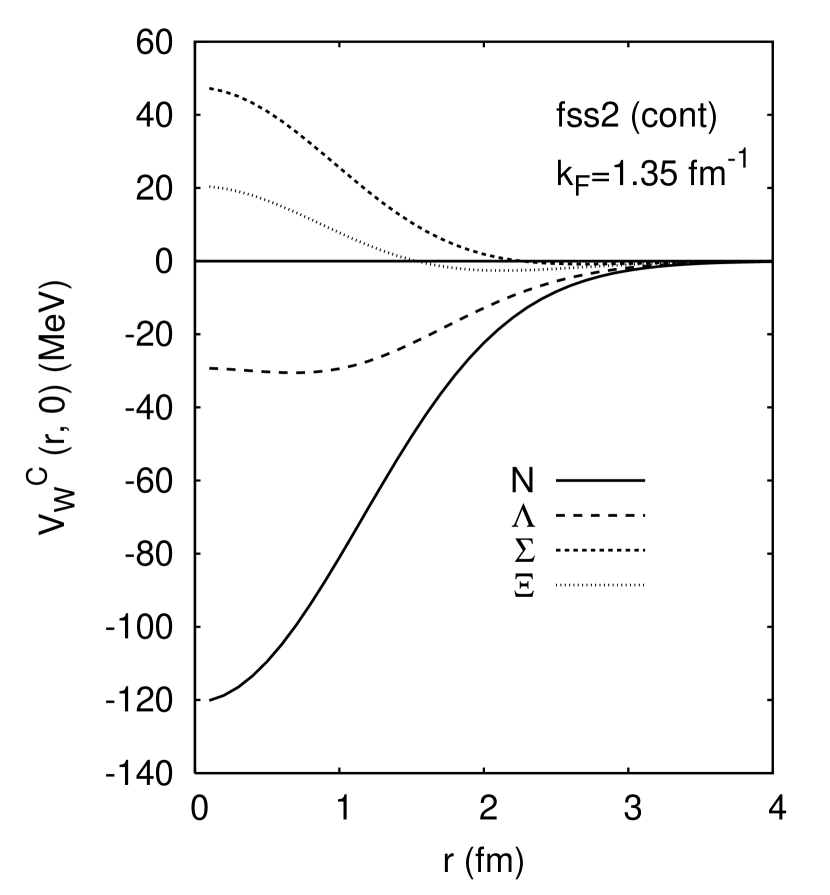
Figure 1: The central component of the zero-momentum Wigner transform ${V_{W}}^{C}(r,0)$ for the $B_{8}\alpha$ Born kernel, calculated from the quark-model $G$-matrix $B_{8}B_{8}$ interactions by fss2. The Fermi momentum used in the $G$-matrix calculation is $k_{F}=1.35~{}\hbox{fm}^{-1}$ and the continuous choice is used for intermediate spectra. The $(0s)^{4}$ shell-model wave function with the h.o. size parameter $\nu=0.257~{}\hbox{fm}^{-2}$ is used for the $\alpha$ cluster.

Figure 2: The same as Fig. 2, but for the $LS$ component ${V_{W}}^{LS}(r,0)$.

3 Results and discussion

3.1 $\Lambda\alpha$ interaction

In order to gain the overview of the zero-momentum Wigner transform given in Eq. (LABEL:fm4-5), we will show in Fig. 2 the central ($V^{C}_{W}(\mbox{\boldmath$r$},0)$) and $LS$ ($V^{LS}_{W}(\mbox{\boldmath$r$},0)$) components for the $B_{8}\alpha$ interaction with $B_{8}=N,~{}\Lambda,~{}\Sigma$ and $\Xi$, when the quark-model $G$-matrix $B_{8}B_{8}$ interaction by fss2 are employed with the continuous choice for intermediate spectra. In this case, we choose $q_{1}=0$ and the relative momentum $q$ is assigned to the integral mesh point $q$ in Eq. (LABEL:fm4-5). The Fermi-momentum used for the $G$-matrix calculation is $k_{F}=1.35~{}\hbox{fm}^{-1}$, and the $(0s)^{4}$ shell-model wave function with the h.o. size parameter $\nu=0.257~{}\hbox{fm}^{-2}$ is used for the $\alpha$-cluster folding. We note that the correct treatment of the total c.m. motion for the $B_{8}\alpha$ system is very important, since the c.m. correction in the standard approach is of the order of $1/A\sim 1/4$. As the result, the zero-momentum Wigner transform becomes very much short-ranged and deep with the interaction range about $R=1.2A^{1/3}\sim 2~{}\hbox{fm}$. The $\alpha$-particle density in Eq. (2.74) is more compact than the density including the c.m. motion, $\rho(r)=4(2\nu/\pi)^{3/2}\,e^{-2\nu r^{2}}$, and the central density is about $(4/3)^{3/2}\sim 1.5$ times larger. The extremely large $N\alpha$ Wigner transform in Fig. 2 is because of the factor 2 in Eq. (A.9), and also because the other nucleon-exchange term than the knock-on term and the effect of the exchange normalization kernel are neglected. We will deal with this case in a separate paper.

Table 1: Values of the zero-momentum Wigner transform at the origin $\mbox{\boldmath$r$}=0$, $V^{C}_{W}(0,0)$ and $V^{LS}_{C}(0,0)$, and the Scheerbaum-like factor, $\widetilde{S}_{B}$, in Eq. (2.77). The unit is in MeV for $V^{C}_{W}(0,0)$ and $V^{LS}_{C}(0,0)$, and in MeV $\hbox{fm}^{5}$ for $\widetilde{S}_{B}$. The models are fss2 and FSS, and $qtq$ and cont. imply the $QTQ$ and continuous choices for intermediate spectra, respectively, used in the $G$-matrix calculations.

	$B$	FSS		fss2
		$qtq$	cont	$qtq$	cont
	$N$	$-112.8$	$-121.1$	$-112.6$	$-120.0$
$V^{C}_{W}(0,0)$	$\Lambda$	$-26.01$	$-26.03$	$-28.09$	$-29.31$
	$\Sigma$	59.33	48.72	51.76	47.24
	$\Xi$	7.97	10.73	20.83	20.38
	$N$	$-65.60$	$-67.65$	$-63.89$	$-65.31$
$V^{LS}_{W}(0,0)$	$\Lambda$	$-14.56$	$-14.70$	$-17.89$	$-18.91$
	$\Sigma$	$-28.07$	$-23.45$	$-24.32$	$-22.92$
	$\Xi$	18.59	25.55	7.71	8.59
	$N$	$-51.00$	$-52.24$	$-52.15$	$-53.49$
$\widetilde{S}_{B}$	$\Lambda$	$-5.32$	$-5.04$	$-13.22$	$-13.96$
	$\Sigma$	$-34.87$	$-30.36$	$-31.69$	$-30.89$
	$\Xi$	20.15	26.30	6.77	7.62

We list in Table 1 the values of the zero-momentum Wigner transform at the origin $\mbox{\boldmath$r$}=0$, and the Scheerbaum-like factor $\widetilde{S}_{B}$ in Eq. (2.77) for all the possible combinations of $G$-matrix calculations for the models, fss2 and FSS, and for the $QTQ$ and continuous choices for intermediate spectra. The corresponding values for the single-particle potentials, $U_{B}(q_{1})$, and the Scheerbaum factors, $S_{B}(q_{1})$, at $q_{1}=0$ in symmetric nuclear matter with $k_{F}=1.35~{}\hbox{fm}^{-1}$ are listed in Table 2. By comparing these results, we obtain the following findings:

1. The $\Lambda\alpha$ central Wigner transforms are fairly shallow in comparison with $U_{\Lambda}(0)$ in the symmetric nuclear matter calculations. Namely, $|V^{C}_{W}(0,0)|$ is less than 30 MeV in all the cases, while $|U_{\Lambda}(0)|$ is more than 40 MeV.

2. The $\Sigma\alpha$ and $\Xi\alpha$ central Wigner transforms are repulsive, although $U_{\Xi}(0)$ is attractive. In particular, $V^{C}_{W}(0,0)$ for $\Sigma\alpha$ is strongly repulsive, which is due to the quark-model prediction of the repulsive $\Sigma N(I=3/2)$ ${}^{3}S_{1}$ interaction. These characters are the result of strong isospin dependence of the $\Sigma N$ and $\Xi N$ interactions, which is discussed in the next subsection.

3. The $LS$ component, $V^{LS}_{W}(0,0)$, for the $\Lambda\alpha$ interaction is by no means extremely small, in comparison with that for the $\Sigma\alpha$ interaction. The ratio is only 70 – 80 % for fss2 and 50 – 60 % for FSS. On the other hand, $\widetilde{S}_{B}$ factors reflect the characteristics of $S_{B}(0)$; namely, $\widetilde{S}_{B}$ is about 20 – 30 % larger than $S_{B}(0)$, which is about equal to the enhancement factor $\frac{1+4\xi}{4\xi}\sim 1.25$ – 1.35 in Eqs. (2.77) and (2.81).

Table 2: The depth of the single-particle potentials, $U_{B}(q_{1})$, and the Scheerbaum factors, $S_{B}(q_{1})$, at $q_{1}=0$ obtained by the angular-averaged $G$-matrix calculations of the quark-model potentials in symmetric nuclear matter. The Fermi-momentum $k_{F}=1.35~{}\hbox{fm}^{-1}$ is used. The models are fss2 and FSS, and $qtq$ and cont. imply the $QTQ$ and continuous choices for intermediate spectra, respectively.

	$B$	FSS		fss2
		$qtq$	cont	$qtq$	cont
	$N$	$-79.8$	$-89.3$	$-80.6$	$-88.9$
$U_{B}(0)$	$\Lambda$	$-42.9$	$-46.3$	$-44.8$	$-48.4$
	$\Sigma$	16.1	17.3	9.5	7.3
	$\Xi$	$-14.9$	$-20.8$	$-5.3$	$-8.0$
	$N$	$-40.3$	$-41.4$	$-41.3$	$-42.4$
$S_{B}(0)$	$\Lambda$	$-3.9$	$-3.6$	$-10.0$	$-10.6$
	$\Sigma$	$-27.4$	$-22.6$	$-24.1$	$-23.2$
	$\Xi$	14.6	21.4	4.6	5.8

Figure 3: Solutions of the transcendental equation Eq. (3.3), obtained from the $\Lambda\alpha$ Wigner transform for the various effective $\Lambda N$ potentials. SB is the Sparenberg-Baye potential, Eqs. (3.1) and (3.2), NSC, ND, NF are the simulated versions of the Nijmegen potentials, and JA, JB are those of the Jülich potentials. The energy $E=-3.12$ MeV is assumed. The $(0s)^{4}$ shell-model wave function with the h.o. size parameter $\nu=0.257~{}\hbox{fm}^{-2}$ is used for the $\alpha$-cluster.

Figure 4: The same as Fig. 4, but for the Wigner transform, $V^{C}_{W}(\mbox{\boldmath$r$},\mbox{\boldmath$q$})$ in Eq. (2.66), calculated from the quark-model $G$-matrix interactions. The $\Lambda\alpha$ Born kernels are calculated from the quark-model $G$-matrix $B_{8}B_{8}$ interactions by fss2 and FSS. The Fermi momentum used in the $G$-matrix calculation is $k_{F}=1.35~{}\hbox{fm}^{-1}$, and $qtq$ stands for the $QTQ$ prescription and cont for the continuous choice for intermediate spectra.

We find that the zero-momentum Wigner transform is not good enough to define phase-shift equivalent local potentials, especially for the $\Lambda\alpha$ interaction, In order to see this clearly, we examined the Wigner transform for several effective $\Lambda\alpha$ potentials, which can be easily derived from the $\Lambda\alpha$ Born kernels given in Appendix B of Ref. [7]. The effective $\Lambda N$ potentials we examined are the Sparenberg-Baye potential (SB potential) [7] given by

$$v_{\Lambda N}=\left[\,v({}^{1}E)\frac{1-P_{\sigma}}{2}+v({}^{3}E)\frac{1+P_{\sigma}}{2}\,\right]\,\left[\,\frac{u}{2}+\frac{2-u}{2}P_{r}\,\right]\ ,$$ (3.1)

with

$$v({}^{1}E) = -128.0~{}\exp(-0.8908~{}r^{2})+1015~{}\exp(-5.383~{}r^{2})\ ,$$

$$v({}^{3}E) = -56.31\,f\,\exp(-0.7517~{}r^{2})+1072~{}\exp(-13.74~{}r^{2})\ ,$$ (3.2)

and the $G$-matrix simulated $\Lambda N$ forces [18] generated from the various OBEP potentials, NS (Nijmegen soft-core model NSC89), ND (hard-core model D) , NF (hard-core model F), JA (Jülich model A), and JB (model B). By choosing the parameters, $u=0.94687$ and $f=0.8923$ in Eqs. (3.1) and (3.2), we can correctly reproduce the $\Lambda$ separation energy in ${}^{5}_{\Lambda}\hbox{He}$: $E^{\rm exp}_{B}({}^{5}_{\Lambda}\hbox{He})=-3.12\pm 0.02~{}\hbox{MeV}$. The strength of the short-range repulsive term (the third component) of the NS - JB potentials are slightly modified from the original values, in order to reproduce this value. (See Ref. [7].) The phase-shift equivalent local potential in the semi-classical WKB-RGM approximation [32, 33, 30] is calculated by solving the transcendental equation

$$U_{\rm eff}(R)=G^{W}\left(R\,,~{}\sqrt{(2\mu_{\Lambda\alpha}/\hbar^{2})\left[E-U_{\rm eff}(R)\right]}\right)\ \ ,$$ (3.3)

for some specific energies $E$, where $G^{W}(R,\,q)$ is assigned to $V^{C}_{W}(\mbox{\boldmath$r$},\mbox{\boldmath$q$})$ in Eq. (2.66) with $R=r=|\mbox{\boldmath$r$}|$ and $q=|\mbox{\boldmath$q$}|$. We here study only the $S$ wave, by neglecting the usual semi-classical centrifugal term $\hbar^{2}(\ell+1/2)^{2}/2\mu_{\Lambda\alpha}$. The centrifugal potentials are included only in the Schrödinger equation. This is a plausible approximation, since the $LS$ term of the $\Lambda\alpha$ interaction is very small. The obtained $\Lambda\alpha$ effective local potentials with $E=-3.12~{}\hbox{MeV}$ are plotted in Fig. 4 for SB - JA potentials. The depth of $U_{\rm eff}$ is tabulated in Table 3, together with the $q^{2}$ value at $R=0$, determined self-consistently. The bound-state energy of this effective local potential, $E_{B}$, is calculated by solving the Schrödinger equation

$$\left[-\frac{\hbar^{2}}{2\mu_{\Lambda\alpha}}\frac{\partial^{2}}{(\partial R)^{2}}+U_{\rm eff}(R)\right]\Psi(R)=E_{B}\,\Psi(R)\ \ .$$ (3.4)

We find that the bound-state energies of SB - JA potentials are too small, compared with the exact value $E_{B}({\rm exact})$, which is obtained by solving the Lippmann-Schwinger equation using the $\Lambda\alpha$ Born kernels. Namely, $E_{B}$ from $U_{\rm eff}(R)$ is from 1.3 MeV to 1.7 MeV too small in magnitude, except for the rather moderate difference 0.74 MeV in ND. Figure 4 shows that this difference is related with the interaction range of $U_{\rm eff}(R)$; i.e., the range of ND is long while the others are short. This poor result of the WKB-RGM approximation for the $\Lambda\alpha$ interaction is probably related to the very strong nonlocality (or momentum dependence) originating from the $P_{r}$ term in Eq. (3.1). In order to see this, we artificially changed the Majorana exchange mixture parameter $u$ in Eq. (3.1) and compared $E_{B}$ obtained by the Wigner transform technique and by the exact method using the $\Lambda\alpha$ Born kernel. Table 4 shows this comparison. The case $u=2$ corresponds to pure Wigner-type $\Lambda\alpha$ interaction, which gives a local $\Lambda\alpha$ potential and complete agreement between the two methods. Once we decrease the $u$ value and introduce the Majorana component, the Wigner transform technique loses the attractive effect of nonlocality very much and eventually reaches at a very weak effective local potential with no bound state before $u=0$ (the strength of the odd force =$-$(the strength of the even force)). Our case is just in the middle of these two extremes, which corresponds to the approximate Serber-type interaction with a weak odd force. On the other hand, the exact solution is almost independent of the $u$ value, which implies that the $\Lambda$-particle is bound to the $\alpha$-cluster in the almost $S$ wave.

Table 3: The depth of the effective local potential $U_{\rm eff}(0)$, obtained by solving the transcendental equation Eq. (3.3) with $E=-3.12$ MeV. The $q^{2}$ value at $R=0$ and a special value $V^{C}_{W}(0,0)$ of the $\Lambda\alpha$ Wigner transform at $\mbox{\boldmath$r$}=0$ and $\mbox{\boldmath$q$}=0$ are also given. The eigenvalue $E_{B}$ is obtained by solving the $S$-wave Schrödinger equation Eq. (3.4) for $U_{\rm eff}(R)$. The heading $E_{B}$ (exact) indicates the exact eigenvalue, calculated from the $\Lambda\alpha$ Born kernel. The quark-model $G$-matrix interactions are fss2 and FSS both in the $QTQ$ ($qtq$) and continuous (cont) prescriptions for intermediate spectra. The depth of the $LS$ potential $U^{LS}_{\rm eff}(0)$ is calculated from the $q^{2}$ value determined by using only the central force.

model	$V^{C}_{W}(0,0)$	$q^{2}$	$U_{\rm eff}(0)$	$U_{\rm eff}^{LS}(0)$	$E_{B}$	$E_{B}$ (exact)
	(MeV)	(fm-2)	(MeV)	(MeV)	(MeV)
SB	$-58.86$	1.062	$-27.15$		$-1.86$	$-3.12$
NS	$-71.00$	1.269	$-31.85$		$-1.74$	$-3.12$
ND	$-32.08$	0.613	$-16.98$		$-2.38$	$-3.12$
NF	$-61.91$	0.959	$-24.83$		$-1.78$	$-3.12$
JA	$-74.35$	1.168	$-29.56$		$-1.60$	$-3.12$
JB	$-83.71$	1.312	$-32.81$		$-1.43$	$-3.12$
fss2 (cont)	$-29.53$	0.731	$-19.66$	$-17.22$	$-2.94$	$-3.62$
fss2 ($qtq$)	$-28.04$	0.657	$-17.99$	$-16.24$	$-2.15$	$-2.75$
FSS (cont)	$-26.35$	0.673	$-18.34$	$-11.50$	$-2.62$	$-3.18$
FSS ($qtq$)	$-25.95$	0.607	$-16.87$	$-12.30$	$-1.78$	$-2.29$

Table 4: Comparison of the $S$-wave bound-state energies calculated from the Wigner transform technique ($E_{B}$) and the Lippmann-Schwinger approach of the $\Lambda\alpha$ Born kernel ($E_{B}({\rm exact})$), when the Majorana exchange parameter $u$ in Eq. (3.1) is changed from $u=2$ (pure Wigner) to $u=0$ (pure Majorana).

$u$	$E_{B}$	$E_{B}$ (exact)
	(MeV)	(MeV)
2	$-3.219$	$-3.219$
1	$-1.864$	$-3.120$
0.5	$-1.272$	$-3.079$
0	unbound	$-3.041$

Figure 5: The central component of the zero-momentum Wigner transform, $V^{C}_{W}(R,0)$, and the solution of the transcendental equation, $U_{\rm eff}(R)$, for the quark-model $G$-matrix interaction fss2. The continuous choice for intermediate spectra is used for the $G$-matrix calculation.

Figure 6: The same as Fig. 6, but for the $LS$ component. The local momentum $q$ is determined self-consistently by using only the central components as in Fig. 6.

Figure 7: The same as Fig. 4 but for the $LS$ components. The local momentum is determined only by the central force.

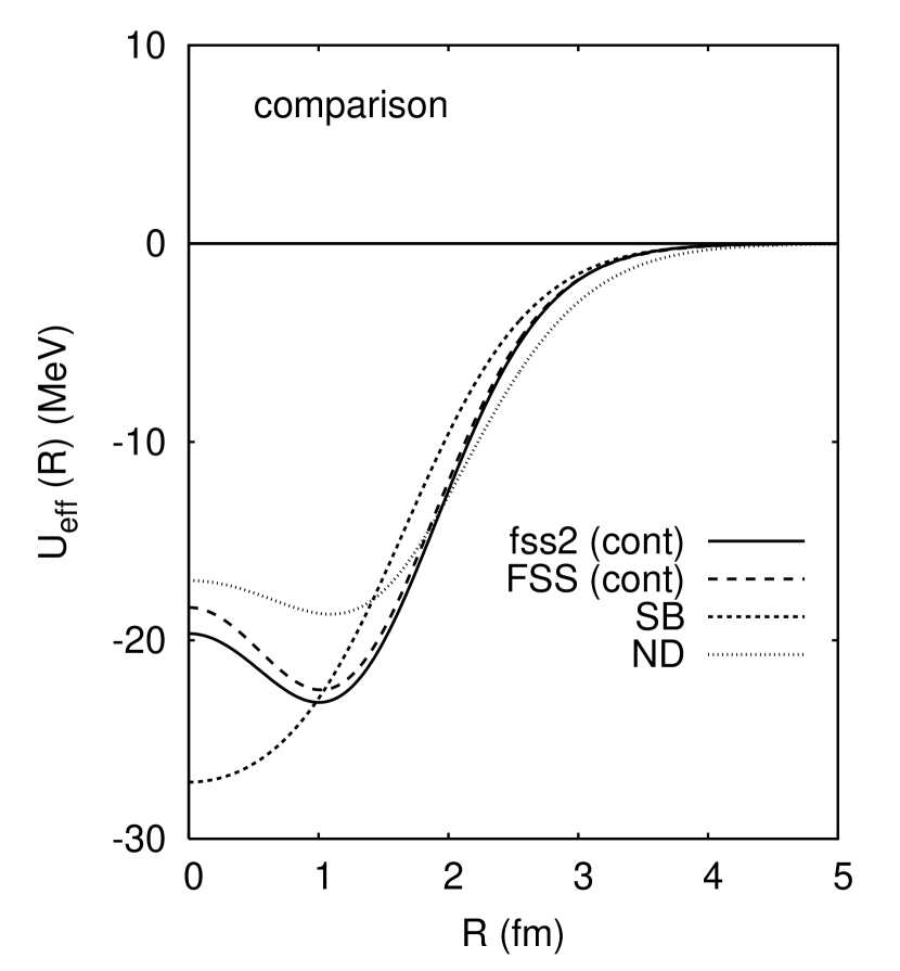
Figure 8: Comparison of effective local potentials predicted by the quark-model $G$-matrix interactions fss2, FSS (with the continuous choice for intermediate spectra) and by some of the effective $\Lambda N$ forces, SB and ND potentials.

The situation is almost the same even with the Wigner transform approach of the quark-model $G$-matrix interaction. We show in Fig. 4 solutions of the transcendental equations obtained from the Wigner transform of $\Lambda\alpha$ Born kernels. Here we also assumed $E=-3.12$ MeV. We find that different prescriptions for the $G$-matrix calculations, the $QTQ$ ($qtq$) or the continuous (cont) choice for intermediate spectra, give essentially same result with a slightly smaller attraction for the $QTQ$. The model FSS gives a little weaker attraction than fss2. The bound-state energies listed in Table 3 show that the Schrödinger equation of $U_{\rm eff}(R)$ gives smaller energies by 0.5 $\sim$ 0.7 MeV than the exact method using the $\Lambda\alpha$ Born kernel. In fact, the bound-state energy for ${}^{5}_{\Lambda}\hbox{He}$, obtained by solving the Lippmann-Schwinger equation is $-3.62$ MeV for fss2 (cont) and $-3.18$ MeV for FSS (cont). These values are by no means too large, compared with the experimental value $E^{\rm exp}_{B}({}^{5}_{\Lambda}\hbox{He})=-3.12\pm 0.02~{}\hbox{MeV}$. Table 3 also shows that the attraction is reduced when the zero-momentum Wigner transform is converted to the effective local potential. This is depicted in Fig. 6 for a typical example of the fss2 prediction with the continuous prescription. The small difference of $V^{C}_{W}(0,0)$ values in Table 3 from those in Table 1 is because $r=0.1~{}\hbox{fm}$ and $q=0.013~{}\hbox{fm}^{-1}$ are actually used in Table 1, instead of $r=q=0$, and also because a spline interpolation for $q$ is applied to ${\mathcal{V}}^{C}_{0}(k,q)$ in Eq. (2.66), to facilitate the Wigner transform for an arbitrary $q$. The $LS$ component $U_{\rm eff}^{LS}(R)$ depicted in Figs. 6 and 8, and the depth $U_{\rm eff}^{LS}(0)$ in Table 3 are calculated from the $LS$ Wigner transform in Eq. (2.66) by using local momentum $q$ determined self-consistently for each $R$, with respect to the central component. First we find in Fig. 6 that the modification of the zero-momentum $LS$ Wigner transform to the effective local potential is comparatively small. Secondly, Fig. 8 shows that the model FSS gives a shallower $LS$ potential than model fss2, which is a result of the strong cancellation between the ordinary $LS$ and the antisymmetric $LS$ ($LS^{(-)}$) forces in the model FSS. In Fig. 8, we compare the central components of the effective local potentials obtained by the quark-model $G$-matrix interaction and by some of the effective $\Lambda N$ forces. We find that the $G$-matrix prediction is rather long-ranged and situated in the middle of ND and SB predictions. The shape of our $\Lambda\alpha$ central potential is rather similar to one of the phenomenological potentials in Ref. [19] (B of Fig. 5), and to the effective potential derived from a five-particle microscopic wave function with hard core correlations in Ref. [20] (the dashed curve of Fig. 6). It is convenient to parametrize the obtained $\Lambda\alpha$ potentials in simple Gaussian functions. For example, the effective local potential at $E=-3.12$ MeV, predicted by fss2 (cont) in Fig. 8, is expressed as

$$U(R)=-(19.42+19.50\,R^{2})\,e^{-0.5145\,R^{2}}\ \ (\hbox{MeV})\ \ ,$$ (3.5)

with the bound-state energy $E_{B}=-2.95$ MeV (which corresponds to $-2.94$ MeV in Table 3).

Table 5: The depths of the effective local potentials, $U_{\rm eff}(0)$, and the $S$-wave phase shifts, $\delta^{W}_{0}(E)$, obtained by solving the Schrödinger equation. The exact phase shift, $\delta_{0}(E)$ (exact), is also shown, which is obtained by solving the Lippmann-Schwinger equation from the Born kernel.

model	$E_{\rm c.m.}$	$U_{\rm eff}(0)$	$\delta^{W}_{0}(E)$	$\delta_{0}(E)$ (exact)
	(MeV)	(MeV)	(deg)	(deg)
	10	$-20.74$	62.74	72.20
SB	30	$-11.90$	29.01	36.28
	50	$-4.26$	15.37	20.69
	10	$-25.16$	61.67	72.88
NS	30	$-15.58$	28.12	37.10
	50	$-6.74$	13.46	20.46
	10	$-10.69$	62.14	68.39
ND	30	$-1.78$	26.89	32.90
	50	6.29	12.83	17.94
fss2	10	$-15.33$	70.58	74.82
(cont)	30	$-9.46$	36.24	40.54
	50	$-4.04$	22.47	25.75
fss2	10	$-13.18$	64.92	70.07
(qtq)	30	$-6.63$	31.28	35.50
	50	$-1.09$	18.18	21.54
FSS	10	$-14.60$	69.70	73.49
(cont)	30	$-9.79$	36.88	40.50
	50	$-4.96$	23.01	26.62
FSS	10	$-12.21$	62.64	67.88
(qtq)	30	$-6.10$	30.25	34.30
	50	$-1.27$	18.14	21.20

We list in Table 5 the depths of the effective local potentials $U_{\rm eff}(0)$ for positive energies, $E_{\rm c.m.}=10,~{}30$ and 50 MeV, and the $S$-wave phase shifts $\delta^{W}_{0}(E)$ obtained by solving the Schrödinger equation. The exact phase shift $\delta_{0}(E)$ (exact) is also shown, which is obtained from the Born kernel. Here we again find the effective local potentials are too shallow, especially for the effective $\Lambda N$ forces. The phase shift difference is about 5 - $11^{\circ}$ for the effective $\Lambda N$ forces, while 3 - $5^{\circ}$ for the quark-model $G$-matrix interactions. This implies that we need a readjustment of the effective local potentials of the order of 10 MeV, in order to reproduce the correct magnitude of the phase shifts.

Finally, we will make a brief comment on the choice of the $k_{F}$ value in the present framework. If we choose a smaller $k_{F}$, the $\Lambda$ s.p. potential in the symmetric nuclear matter becomes shallower and the $\Lambda\alpha$ central interaction becomes more attractive. The first feature reduces the magnitude of the starting energy in the $\Lambda N$ $G$-matrix, resulting in more attractive $\Lambda N$ $G$-matrix. Although this change is compensated by the smaller volume in the phase-space integral to calculate the $\Lambda$ s.p. potential, such a mechanism does not work in the present calculation of the $\Lambda\alpha$ interaction. Thus the $\Lambda\alpha$ central interaction after the $\alpha$-cluster folding becomes more attractive for a smaller $k_{F}$. The same situation is observed in Fig. 4 of Ref. [25] for their $\Sigma(3N)$ potential. For example, if we change $k_{F}=1.35~{}\hbox{fm}^{-1}$ to $1.20~{}\hbox{fm}^{-1}$ (which corresponds to the 70$\%$ of the normal density), the depth of the $\Lambda$ s.p. potential, $U_{\Lambda}(0)$, in Table 2 is reduced from $-48.4$ MeV to $-37.5$ MeV for the model fss2 in the continuous choice. On the other hand, the depth of the effective local potential, $U_{\rm eff}(0)$, and $E_{B}({\rm exact})$ in Table 3 changes from $-19.66$ MeV to $-21.74$ MeV and from $-3.62$ MeV to $-4.54$ MeV, respectively. This implies that the self-consistent mechanism of the starting-energy dependence, which is not properly taken into account in this paper, is in fact very important. This finding is in accord with the importance of the Brueckner rearrangement effect discussed in Ref. [14]. Since the purpose of the present study is not to examine the change of the $\alpha$-cluster, it would be safe to assume the standard value $k_{F}=1.35~{}\hbox{fm}^{-1}$, in order to examine the qualitative features of the $B_{8}\alpha$ interaction.

3.2 $\Sigma\alpha$ and $\Xi\alpha$ interactions

Figure 9: The central components of the zero-momentum Wigner transform, ${V_{W}}^{C}(\mbox{\boldmath$r$},0)$ with $R=|\mbox{\boldmath$r$}|$, for the $\Sigma\alpha$ Born kernel, calculated from the quark-model $G$-matrix $B_{8}B_{8}$ interactions by FSS. The Fermi momentum $k_{F}=1.35~{}\hbox{fm}^{-1}$ and the continuous choice are used for the $G$-matrix calculation. The h.o. size parameter $\nu=0.257~{}\hbox{fm}^{-2}$ is used for the $\alpha$-cluster.

Figure 10: The same as Fig. 10, but for fss2.  

As seen from Fig. 2, the $\Sigma\alpha$ and $\Xi\alpha$ interactions are repulsive. This does not mean that the $\Sigma$ and $\Xi$ potentials are always repulsive. The structure of spin-isospin factors for the $\Sigma\alpha$ and $\Xi\alpha$ systems is especially simple (see Eq. (2.15)), which is due to the spin-isospin saturated character of the $\alpha$-particle. It is, therefore, important to examine each isospin component separately, in order to gain some insight to other possibilities of unknown hypernuclei. Here we discuss some qualitative features of these interactions, based on the symmetry properties of the $B_{8}B_{8}$ interactions predicted by the quark-model interactions, FSS and fss2. When the interaction is repulsive, the transcendental equation Eq. (3.3) sometimes does not have its solution, since the square of the local momentum, $q^{2}$, becomes negative. Since the extension of the Wigner transform Eq. (2.66) to the negative $q^{2}$ is not easy numerically, we only discuss the zero-momentum Wigner transform in this subsection.

Figure 11: The same as Fig. 10, but for the $LS$ components.

Figure 12: The same as Fig. 12, but for fss2.

Figures 10 and 10 show the isospin components with $I=1/2$ and $I=3/2$ for the $\Sigma\alpha$ central interaction, predicted by FSS and fss2, respectively. We find that both interactions have some amount of attraction originating from the ${}^{3}S_{1}$ channel of the $I=1/2$ $\Sigma N$ interaction. This channel becomes attractive due to the very strong $\Lambda N$–$\Sigma N$ coupling by the one-pion exchange tensor force. On the other hand, the ${}^{3}S_{1}$ state of the $I=3/2$ channel is strongly repulsive due to the Pauli principle at the quark level. We find from Figs. 10 and 10 that this repulsion is so strong that almost no attraction from the $I=1/2$ channel remains in the $\Sigma\alpha$ interaction.

Figure 13: The same as Fig. 10, but for the $\Xi\alpha$ interaction.

Figure 14: The same as Fig. 14, but for fss2.

Figure 15: The same as Fig. 14, but for the $LS$ components.

Figure 16: The same as Fig. 16, but for fss2.

On the other hand, the two isospin channels, $I=1/2$ and 3/2, yield fairly large $LS$ force for the $\Sigma\alpha$ interaction. This can be seen in Figs. 12 and 12. In the isospin $I=3/2$ channel, ${}^{3}P_{J}$ states are classified to the flavor symmetric channel with the $SU_{3}$ label (22). It is, therefore, plausible that the same mechanism as the $NN$ $I=1$ channel yields very strong $LS$ force. On the other hand, a part of the $LS$ force from the isospin $I=1/2$ channel is due to the flavor-exchange process between $(11)_{a}$ and $(11)_{s}$ $SU_{3}$ configurations. This process is accompanied with the spin flip between $S=0$ and 1, and yields very strong $LS^{(-)}$ force. The $LS$ and $LS^{(-)}$ forces reinforce each other in just opposite way to the $\Lambda N$ interaction, and the resultant $\Sigma\alpha$ $LS$ force becomes almost 3/5 of the $N\alpha$ $LS$ force, as seen from $\widetilde{S}_{B}$ in Table 1. This ratio is almost the same as that of the Scheerbaum factors $S_{B}=S_{B}(0)$ in symmetric nuclear matter. (See Table 2.)

Figures 14 and 14 show the isospin components with $I=0$ and $I=1$ for the $\Xi\alpha$ central interaction, predicted by FSS and fss2, respectively. Here again we find the situation that the attractive nature of the $I=0$ component is largely canceled by the repulsion in the $I=1$ channel. However, this cancellation is not strong especially in the model FSS, and we have almost 5 MeV attraction around $R=2$ fm. In fss2, the height of the central repulsion in the $I=1$ channel is almost 20 MeV, and we can expect a few MeV attraction in the surface region. These long-range attractions may have some influence to the atomic orbit between $\Xi^{-}$ and $\alpha$. The $\Xi\alpha$ potential rather similar (though more attractive) to that by FSS is presented by Myint and Akaishi in Ref. [26]. It should be noted that the origin of the repulsion in the $I=1$ channel is the Pauli forbidden state $(11)_{s}$ in the ${}^{1}S_{0}$ state and the almost Pauli forbidden state (30) in the ${}^{3}S_{1}$ state. However, the coupling with the $\Lambda\Sigma$ channel is very important, which may cause the long-range attraction even in the $I=1$ channel.

The $LS$ components of the $\Xi\alpha$ interaction is repulsive, which is clearly seen in Figs. 16 ans 16. This $LS$ force is fairly strong, especially for FSS. The magnitude is almost 1/3 of the $N\alpha$ $LS$ force with the opposite sign. These features are very similar to the $LS$ force in symmetric nuclear matter, as seen in Table 2.

4 Summary

The $SU_{6}$ quark-model baryon-baryon interaction (fss2, FSS) [1, 2, 3] is a unified model which describes all the baryon-octet baryon-octet ($B_{8}B_{8}$) interactions in a full coupled-channel formalism. For the nucleon-nucleon ($NN$) and hyperon-nucleon ($YN$) interactions, all the available experimental data are reasonably reproduced. It is, therefore, interesting to study $B_{8}\alpha$ interactions in a microscopic framework under a simple assumption of the $(0s)^{4}$ harmonic-oscillator shell-model wave function for the $\alpha$-cluster. In this study, we have used the result of $G$-matrix calculations for symmetric nuclear matter, as an input for the two-body interactions for the $\alpha$-cluster folding. Since the resultant $B_{8}\alpha$ interactions are rather insensitive to the Fermi-momentum $k_{F}$ in the $G$-matrix calculations (except for the $\Lambda N$ $LS$ force for FSS), we have assumed $k_{F}=1.35~{}\hbox{fm}^{-1}$. The other $G$-matrix parameters, the center-of-mass (c.m.) momentum $K$ of two interacting particles and the starting energy $\omega$, are treated unambiguously in the total c.m. frame of the $B_{8}\alpha$ system. This can be achieved by considering the transformation of the matrix elements in the momentum representation from the initial ($\mbox{\boldmath$q$}_{i}$) and final ($\mbox{\boldmath$q$}_{f}$) momenta to the momentum transfer ($\mbox{\boldmath$k$}=\mbox{\boldmath$q$}_{f}-\mbox{\boldmath$q$}_{i}$) and the local momentum $\mbox{\boldmath$q$}=(\mbox{\boldmath$q$}_{f}+\mbox{\boldmath$q$}_{i})/2$. If one uses this transformation at the level of $G$-matrix, the procedure of the $\alpha$-cluster folding becomes extremely simple both for the central and $LS$ components. The $B_{8}\alpha$ interaction, ${\mathcal{V}}^{\Omega}(\mbox{\boldmath$k$},\mbox{\boldmath$q$})$ with $\Omega=C,~{}LS$, represented by $k$ and $q$ is then transformed back to the $B_{8}\alpha$ Born kernel, $V^{\Omega}(\mbox{\boldmath$q$}_{f},\mbox{\boldmath$q$}_{i})$, through the inverse transformation. This procedure is also convenient to calculate the Wigner transform, $V^{\Omega}_{W}(\mbox{\boldmath$r$},\mbox{\boldmath$q$})$, which is simply a Fourier transform of ${\mathcal{V}}^{\Omega}(\mbox{\boldmath$k$},\mbox{\boldmath$q$})$. By solving the transcendental equation for $V^{\Omega}_{W}(\mbox{\boldmath$r$},\mbox{\boldmath$q$})$, we can obtain an energy-dependent local potential of the $B_{8}\alpha$ system in the WKB-RGM approximation [32, 33, 30].

In this paper, we have applied the present formalism to the $\Lambda\alpha$, $\Sigma\alpha$ and $\Xi\alpha$ systems. Applications to the $N\alpha$ system will be discussed in a separate paper, since this system involves an extra nucleon-exchange term, in addition to the direct and knock-on terms. In the $\Lambda\alpha$ system, the WKB-RGM approximation is rather poor due to the very strong momentum dependence of the exchange knock-on term. This term appears even for the effective $\Lambda N$ force, which is traced back to the strangeness exchange processes. We find that the $\Lambda\alpha$ central potentials predicted by various quark-model $G$-matrices are very similar to each other, irrespective of a specific model, fss2 or FSS, and the $QTQ$ or continuous choice for intermediate spectra. At the bound-state energy, $E=-3.12$ MeV, they are long-range local potentials with the wine-bottle shape, having the depth less than 30 MeV. They are very similar to the $\Lambda\alpha$ potential obtained from the effective $\Lambda N$ potential ND [18], simulating the Nijmegen hard-core model D. The $\Lambda\alpha$ bound-state energies are calculated by solving the Lippmann-Schwinger equation of the $\Lambda\alpha$ Born kernel. These are $-3.62$ MeV for fss2 (cont) and $-3.18$ MeV for FSS (cont), when $k_{F}=1.35~{}\hbox{fm}^{-1}$ is used. It should be noted that the depth of the single-particle potential for $\Lambda$ in symmetric nuclear matter is 48 MeV for fss2 (cont) and 46 MeV for FSS (cont) [1]. The fact that the predicted $\Lambda\alpha$ bound-state energies are by no means too large, in comparison with the experimental value $E^{\rm exp}_{B}({}^{5}_{\Lambda}\hbox{He})=-3.12\pm 0.02~{}\hbox{MeV}$, implies that the proper treatment of the c.m. motion of the $\Lambda\alpha$ system is very important. It is also important to note that, in the present $G$-matrix approach, the $\Lambda N$–$\Sigma N$ coupling by the very strong one-pion exchange tensor force is explicitly treated, the lack of which is known to lead to the so-called overbinding problem of the $\Lambda\alpha$ bound state. The energy loss predicted by the $\alpha$-cluster rearrangement effect [14] through the starting-energy dependence of the $G$-matrix needs further detailed analyses. On the other hand, the $\Lambda\alpha$ $LS$ potentials are rather model dependent. In the model fss2, the depth of the $LS$ potential is $-16\sim-17$ MeV, while in FSS about $-12$ MeV. The interaction range of the FSS $LS$ potential is also very short, which leads to a small Scheerbaum-like factor $\widetilde{S}_{\Lambda}$ for the $\Lambda\alpha$ $LS$ force. We will show in a separate paper, the strength of the $LS$ force is further reduced for smaller values of $k_{F}$, if FSS is used. The very small spin-orbit splitting of the ${}^{9}_{\Lambda}\hbox{Be}$ [34, 35] can be reproduced in the $\alpha\alpha\Lambda$ Faddeev calculation, using the $\alpha\alpha$ RGM kernel and the $\Lambda\alpha$ $LS$ Born kernel predicted from the FSS $G$-matrix with $k_{F}=1.25~{}\hbox{fm}^{-1}$.

Based on the reasonable reproduction of the $\Lambda\alpha$ interaction properties, we have examined the real parts of the $\Sigma\alpha$ and $\Xi\alpha$ interactions in the Wigner transform technique. Since these interaction are repulsive, we have examined only the zero-momentum Wigner transform as the first step. In the $\Sigma\alpha$ interaction, the attractive effect from the isospin $I=1/2$ $\Sigma N$ channel is completely cancelled out by the repulsion from the $I=3/2$ $\Sigma N$ channel. The origin of this strong repulsion is the $\Sigma N(I=3/2)$ ${}^{3}S_{1}$ channel, which contains the almost Pauli-forbidden $SU_{3}$ (30) component for the most compact $(0s)^{6}$ configuration. On the other hand, the $\Xi\alpha$ interaction is less repulsive because of the appreciable attraction originating from the $I=0$ $\Xi N$ channels. The $\Xi\alpha$ zero-momentum Wigner transform predicted by FSS yields about $-5$ MeV attraction around $R=2$ fm, while the attraction of fss2 is about $-3$ MeV. These long-range attractions may have some relevance to the formation of atomic bound states for the $\Xi^{-}\alpha$ system. As to the spin-orbit interaction, the two isospin channels of the $\Sigma N$ interaction give fairly strong attractive $\Sigma\alpha$ $LS$ forces, yielding almost 3/5 of the $N\alpha$ $LS$ force. On the other hand, $\Xi\alpha$ $LS$ force is repulsive and the magnitude is $1/8\sim 1/2$ of the $N\alpha$ $LS$ force. We will show in the next paper, the present $N\alpha$ $LS$ force is consistent with the observed $P$-wave splitting of the $3/2^{-}$ and $1/2^{-}$ excited states of ${}^{5}\hbox{He}$.

It should be noted that the overall repulsive character of the $\Sigma\alpha$ and $\Xi\alpha$ interactions is related to the spin-isospin saturated character of the $\alpha$-cluster. The strong isospin dependence of the $\Sigma N$ and $\Xi N$ interactions, namely, repulsive for the $\Sigma N(I=3/2)$ and $\Xi N(I=1)$ channels and attractive for the $\Sigma N(I=1/2)$ and $\Xi N(I=0)$ channels, leads to a possibility of attractive features in some particular spin-isospin channels for systems of $\Sigma$, $\Xi$ and the $s$-shell clusters [23, 24, 25]. One of the examples of such systems is the isospin $I=1/2$ and spin $S=0$ state of ${}^{4}_{\Sigma}\hbox{He}$, in which the strong repulsion of the $\Sigma N(I=3/2)$ ${}^{3}S_{1}$ channel does not contribute [36] and a quasi-bound state is in fact observed experimentally [37, 38]. Applications of the present approach to such systems are under way.

Acknowledgments

This work was supported by Grants-in-Aid for Scientific Research (C) from the Japan Society for the Promotion of Science (JSPS) (Grant Nos. 18540261 and 17540263).

Appendix A Invariant $G$-matrix for the most general $B_{8}B_{8}$ interaction

In this Appendix, we will define the invariant $G$-matrix for the most general $B_{8}B_{8}$ interaction. The $B_{8}B_{8}$ channels in the bra side ($\gamma$) and ket side ($\alpha$) are specified by [30]

$$\gamma = \left[\frac{1}{2}(11)c_{1}\,\frac{1}{2}(11)c_{2}\right]SS_{z}YII_{z};{\mathcal{P}}\ \ ,$$

$$\alpha = \left[\frac{1}{2}(11)a_{1}\,\frac{1}{2}(11)a_{2}\right]S^{\prime}{S_{z}}^{\prime}YII_{z};{{\mathcal{P}}}^{\prime}\ \ ,$$ (A.1)

in the isospin basis. For example, the spin-flavor functions are given by

$$\eta_{\gamma}=\chi_{SS_{z}}\,[B_{1}B_{2}]^{\mathcal{P}}_{II_{z}}\ \ ,$$

$$[B_{1}B_{2}]^{\mathcal{P}}_{II_{z}}=\frac{1}{\sqrt{2(1+\delta_{c_{1},c_{2}})}}\left\{[B_{1}B_{2}]_{II_{z}}+{\mathcal{P}}(-1)^{I_{1}+I_{2}-I}[B_{2}B_{1}]_{II_{z}}\right\}\ ,$$ (A.2)

where the isospin-coupled flavor wave functions, $[B_{1}B_{2}]_{II_{z}}$, are lexicographically ordered and the first baryon is numbered always 1 and the second 2 (i.e., $[B_{2}B_{1}]_{II_{z}}=[B_{2}(1)B_{1}(2)]_{II_{z}}$). The flavor symmetry basis, $[B_{1}B_{2}]^{\mathcal{P}}_{II_{z}}$ with ${\mathcal{P}}=1$ and $-1$, gives

$$\left[B_{1}B_{2}\right]_{II_{z}} = \sqrt{\frac{1+\delta_{c_{1},c_{2}}}{2}}\sum_{\mathcal{P}}\left[B_{1}B_{2}\right]^{\mathcal{P}}_{II_{z}}\ \ ,$$

$$\left[B_{3}B_{4}\right]_{II_{z}} = \sqrt{\frac{1+\delta_{a_{1},a_{2}}}{2}}\sum_{{\mathcal{P}}^{\prime}}\left[B_{3}B_{4}\right]^{{\mathcal{P}}^{\prime}}_{II_{z}}\ \ .$$ (A.3)

The matrix element of the $G$-matrix in the isospin basis and its partial-wave decomposition are given by [31]

$$G_{\gamma\alpha}(\mbox{\boldmath$p$},\mbox{\boldmath$p$}^{\prime};K,\omega) = \langle\chi_{SS_{z}}[B_{1}B_{2}]^{\mathcal{P}}_{II_{z}}|G(\mbox{\boldmath$p$},\mbox{\boldmath$p$}^{\prime};K,\omega)|\chi_{S^{\prime}{S_{z}}^{\prime}}[B_{3}B_{4}]^{{\mathcal{P}}^{\prime}}_{II_{z}}\rangle$$ (A.4)

$$= \sum^{\prime}_{JM\ell\ell^{\prime}}4\pi G^{J}_{\gamma S\ell,\alpha S^{\prime}{S_{z}}^{\prime}}(p,p^{\prime};K,\omega)\sum_{m}\langle\ell mSS_{z}|JM\rangle\,Y_{\ell m}(\widehat{\mbox{\boldmath$p$}})$$

$$\times\sum_{m^{\prime}}\langle\ell^{\prime}m^{\prime}S^{\prime}{S_{z}}^{\prime}|JM\rangle\,Y^{*}_{\ell^{\prime}m^{\prime}}(\widehat{\mbox{\boldmath$p$}}^{\prime})\ \ .$$

Here the prime symbol on $\sum$ implies that the summation is only for such quantum numbers that satisfy the generalized Pauli principle:

$$(-1)^{\ell}(-1)^{1-S}{\mathcal{P}}=(-1)^{\ell^{\prime}}(-1)^{1-S^{\prime}}{\mathcal{P}}^{\prime}=-1\ \ .$$ (A.5)

We multiply Eq. (A.4) with $|\chi_{SS_{z}}\rangle$ and $\langle\chi_{S^{\prime}{S_{z}}^{\prime}}|$ from the left- and right-hand sides, respectively, and take a sum over $SS_{z}$ and $S^{\prime}{S_{z}}^{\prime}$. Then we find

$$\langle[B_{1}B_{2}]^{\mathcal{P}}_{II_{z}}|G(\mbox{\boldmath$p$},\mbox{\boldmath$p$}^{\prime};K,\omega)|[B_{3}B_{4}]^{{\mathcal{P}}^{\prime}}_{II_{z}}\rangle$$

$$=\sum^{\prime}_{JM\ell\ell^{\prime}SS^{\prime}}4\pi\,G^{J}_{\gamma S\ell,\alpha S^{\prime}{S_{z}}^{\prime}}(p,p^{\prime};K,\omega)\,{\mathcal{Y}}_{(\ell S)JM}(\widehat{\mbox{\boldmath$p$}};{\rm spin})\,{\mathcal{Y}}^{*}_{(\ell^{\prime}S^{\prime})JM}(\widehat{\mbox{\boldmath$p$}}^{\prime};{\rm spin})\ \ ,$$

(A.6)

where ${\mathcal{Y}}_{(\ell S)JM}(\widehat{\mbox{\boldmath$p$}};{\rm spin})=[Y_{\ell}(\widehat{\mbox{\boldmath$p$}})\chi_{S}]_{JM}$ is the angular-spin function for the two-baryon system.

Let us denote the two-baryon channels with $c=(c_{1},c_{2})$, $a=(a_{1},a_{2})$, and consider

$$G_{ca}(\mbox{\boldmath$p$},\mbox{\boldmath$p$}^{\prime};K,\omega)$$

$$\equiv\langle[B_{1}B_{2}]_{II_{z}}|G(\mbox{\boldmath$p$},\mbox{\boldmath$p$}^{\prime};K,\omega)-G(\mbox{\boldmath$p$},-\mbox{\boldmath$p$}^{\prime};K,\omega)P_{\sigma}P_{F}|[B_{3}B_{4}]_{II_{z}}\rangle\ \ .$$ (A.7)

We can rewrite this by using Eqs. (A.3) and (A.6):

$$G_{ca}(\mbox{\boldmath$p$},\mbox{\boldmath$p$}^{\prime};K,\omega)$$

$$=\frac{1}{2}\sqrt{(1+\delta_{c_{1},c_{2}})(1+\delta_{a_{1},a_{2}})}\sum_{{\mathcal{P}},{\mathcal{P}}^{\prime}}\left\{\langle[B_{1}B_{2}]^{\mathcal{P}}_{II_{z}}|G(\mbox{\boldmath$p$},\mbox{\boldmath$p$}^{\prime};K,\omega)|[B_{3}B_{4}]^{{\mathcal{P}}^{\prime}}_{II_{z}}\rangle\right.$$

$$\left.-\langle[B_{1}B_{2}]^{\mathcal{P}}_{II_{z}}|G(\mbox{\boldmath$p$},-\mbox{\boldmath$p$}^{\prime};K,\omega)P_{\sigma}P_{F}|[B_{3}B_{4}]^{{\mathcal{P}}^{\prime}}_{II_{z}}\rangle\right\}\ \ .$$ (A.8)

Here the second term in the brackets gives the same contribution as the first term, due to the condition Eq. (A.5). Thus we find that Eq. (A.7) is actually invariant $G$-matrix, which allows the expressions

$$G_{ca}(\mbox{\boldmath$p$},\mbox{\boldmath$p$}^{\prime};K,\omega)$$

$$=\langle[B_{1}B_{2}]_{II_{z}}|G(\mbox{\boldmath$p$},\mbox{\boldmath$p$}^{\prime};K,\omega)-G(\mbox{\boldmath$p$},-\mbox{\boldmath$p$}^{\prime};K,\omega)P_{\sigma}P_{F}|[B_{3}B_{4}]_{II_{z}}\rangle$$

$$=\sqrt{(1+\delta_{c_{1},c_{2}})(1+\delta_{a_{1},a_{2}})}\sum_{{\mathcal{P}},{\mathcal{P}}^{\prime}}\langle[B_{1}B_{2}]^{\mathcal{P}}_{II_{z}}|G(\mbox{\boldmath$p$},\mbox{\boldmath$p$}^{\prime};K,\omega)|[B_{3}B_{4}]^{{\mathcal{P}}^{\prime}}_{II_{z}}\rangle$$

$$=\sqrt{(1+\delta_{c_{1},c_{2}})(1+\delta_{a_{1},a_{2}})}\sum^{\prime}_{JM\ell\ell^{\prime}SS^{\prime}{\mathcal{P}}{\mathcal{P}}^{\prime}}4\pi\,G^{J}_{\gamma S\ell,\alpha S^{\prime}{S_{z}}^{\prime}}(p,p^{\prime};K,\omega)$$

$$\qquad\times{\mathcal{Y}}_{(\ell S)JM}(\widehat{\mbox{\boldmath$p$}};{\rm spin})\,{\mathcal{Y}}^{*}_{(\ell^{\prime}S^{\prime})JM}(\widehat{\mbox{\boldmath$p$}}^{\prime};{\rm spin})$$

$$=\sqrt{(1+\delta_{c_{1},c_{2}})(1+\delta_{a_{1},a_{2}})}\left[g_{0}+g_{ss}\,(\mbox{\boldmath$\sigma$}_{1}\cdot\mbox{\boldmath$\sigma$}_{2})+h_{0}\,i\widehat{\mbox{\boldmath$n$}}\cdot(\mbox{\boldmath$\sigma$}_{1}+\mbox{\boldmath$\sigma$}_{2})\right.$$

$$\left.\qquad+h_{-}\,i\widehat{\mbox{\boldmath$n$}}\cdot(\mbox{\boldmath$\sigma$}_{1}-\mbox{\boldmath$\sigma$}_{2})+\cdots\right]\ \ .$$ (A.9)

The eight independent invariant functions, $g_{0}$, $g_{ss}$, etc., are expressed by some combinations of the partial-wave components of the $G$-matrix, $G^{J}_{\gamma S\ell,\alpha S^{\prime}{S_{z}}^{\prime}}(p,p^{\prime};K,\omega)$, which are explicitly given in Appendix D of Ref. [31].

References

• [1] Y. Fujiwara, Y. Suzuki and C. Nakamoto, Prog. Part. Nucl. Phys. (2006) (in press)
• [2] Y. Fujiwara, M. Kohno, C. Nakamoto and Y. Suzuki, Phys. Rev. C 64 (2001) 054001
• [3] Y. Fujiwara, T. Fujita, M. Kohno, C. Nakamoto and Y. Suzuki, Phys. Rev. C 65 (2002) 014002
• [4] Y. Fujiwara, K. Miyagawa, M. Kohno, Y. Suzuki and H. Nemura, Phys. Rev. C 66 (2002) 021001
• [5] Y. Fujiwara, K. Miyagawa, Y. Suzuki, M. Kohno and H. Nemura, Nucl. Phys. A 721 (2003) 983c
• [6] Y. Fujiwara, K. Miyagawa, M. Kohno and Y. Suzuki, Phys. Rev. C 70 (2004) 024001
• [7] Y. Fujiwara, K. Miyagawa, M. Kohno, Y. Suzuki, D. Baye and J.-M. Sparenberg, Phys. Rev. C 70 (2004) 024002
• [8] Y. Fujiwara, M. Kohno, K. Miyagawa and Y. Suzuki, Phys. Rev. C 70 (2004) 047002
• [9] Y. Fujiwara, M. Kohno, K. Miyagawa, Y. Suzuki and J.-M. Sparenberg, Phys. Rev. C 70 (2004) 037001
• [10] Y. Fujiwara, H. Nemura, Y. Suzuki, K. Miyagawa and M. Kohno, Prog. Theor. Phys. 107 (2002) 745
• [11] Y. Fujiwara, Y. Suzuki, K. Miyagawa, M. Kohno and H. Nemura, Prog. Theor. Phys. 107 (2002) 993
• [12] M. Kohno, Y. Fujiwara, T. Fujita, C. Nakamoto and Y. Suzuki, Nucl. Phys. A 674 (2000) 229
• [13] Y. Fujiwara, M. Kohno, T. Fujita, C. Nakamoto and Y. Suzuki, Nucl. Phys. A 674 (2000) 493
• [14] M. Kohno, Y. Fujiwara and Y. Akaishi, Phys. Rev. C 68 (2003) 034302
• [15] X. Campi and D. W. Sprung, Nucl. Phys. A 194 (1972) 401
• [16] M. Kohno, S. Nagata and N. Yamaguchi, Prog. Theor. Phys. Suppl. No. 65 (1975) 200
• [17] M. Kohno and D. W. L. Sprung, Nucl. Phys. A 397 (1983) 1
• [18] E. Hiyama, M. Kamimura, T. Motoba, T. Yamada and Y. Yamamoto, Prog. Theor. Phys. 97 (1997) 881
• [19] C. Daskaloyannis, M. Grypeos and H. Nassena, Phys. Rev. C 26 (1982) 702
• [20] S. Nakaichi-Maeda and E. W. Schmid, Z. Phys. A 315 (1984) 287
• [21] R. Guardiola and J. Navarro, Acta Phys. Pol. B 24 (1993) 525
• [22] I. N. Filikhin, A. Gal and V. M. Suslov, Phys. Rev. C 68 (2003) 024002
• [23] T. Harada, S. Shinmura, Y. Akaishi and H. Tanaka, Nucl. Phys. A 507 (1990) 715
• [24] S. Okabe, T. Harada and Y. Akaishi, Nucl. Phys. A 514 (1990) 613
• [25] T. Yamada and K. Ikeda, Prog. Theor. Phys. Suppl. No. 117 (1994) 201
• [26] K. S. Myint and Y. Akaishi, Prog. Theor. Phys. Suppl. No. 117 (1994) 251
• [27] C. B. Dover and A. Gal, Prog. Part. Nucl. Phys. 12 (1984) 171
• [28] Th. A. Rijken and Y. Yamamoto, nucl-th/0608074
• [29] R. R. Scheerbaum, Nucl. Phys. A 257 (1976) 77
• [30] C. Nakamoto, Y. Suzuki and Y. Fujiwara, Prog. Theor. Phys. 94 (1995) 65
• [31] Y. Fujiwara, M. Kohno, C. Nakamoto and Y. Suzuki, Prog. Theor. Phys. 103 (2000) 755
• [32] H. Horiuchi, Prog. Theor. Phys. 64 (1980) 184 ; Β K. Aoki and H. Horiuchi, Prog. Theor. Phys. 68 (1982) 1658;Β 2028
• [33] Y. Suzuki and K. T. Hecht, Nucl. Phys. A 420 (1984) 525 ; 446 (1985) 749 (E)
• [34] H. Akikawa et al., Phys. Rev. Lett. 88 (2002) 082501
• [35] H. Tamura et al., Nucl. Phys. A 754 (2005) 58c
• [36] T. Yamada and K. Ikeda, Prog. Theor. Phys. 88 (1992) 139
• [37] R. S. Hayano et al., Phys. Lett. B 231 (1989) 355
• [38] T. Nagae et al., Phys. Rev. Lett. 80 (1998) 1605