Rapidity-dependent spectra from a single-freeze-out model of relativistic heavy-ion collisions

Abstract

An extension of the single-freeze-out model with thermal and geometric parameters dependent on the spatial rapidity, $\alpha_{\parallel}$, is used to describe the rapidity and transverse-momentum spectra of pions, kaons, protons, and antiprotons measured at RHIC at $\sqrt{s_{NN}}=200~{}{\rm GeV}$ by the BRAHMS collaboration. THERMINATOR is used to perform the necessary simulation, which includes all resonance decays. The result of the fit to the rapidity spectra in the range of the BRAHMS data is the expected growth of the baryon and strange chemical potentials with the magnitude of $\alpha_{\parallel}$, while the freeze-out temperature is kept fixed. The value of the baryon chemical potential at $\alpha_{\parallel}\sim 3$, which is the relevant region for particles detected at the BRAHMS forward rapidity $y\sim 3$, is about $200~{}{\rm GeV}$, i.e. lies in the range of the values obtained for the highest SPS energy. The chosen geometry of the fireball has a decreasing transverse size as the magnitude of $\alpha_{\parallel}$ is increased, which also corresponds to decreasing transverse flow. This feature is verified by reproducing the transverse momentum spectra of pions and kaons at various rapidities. The strange chemical potential obtained from the fit to the $K^{+}/K^{-}$ ratio is such that the local strangeness density in the fireball is compatible with zero. The resulting rapidity spectra of net protons are described qualitatively in the model. As a result of the study, the knowledge of the “topography” of the fireball is achieved, making other calculations possible. As an example, we give predictions for the rapidity spectra of hyperons.

I Introduction

The study of particle abundances has been a major source of information concerning heavy-ion collisions. In fact, the agreement of the particle ratios with simple predictions of statistical models is a key argument for early thermalization of the formed system BRAHMS Collab. (2005); PHOBOS Collab. (2005); STAR Collab. (2005); PHENIX Collab. (2005). Up to now the numerous studies of the particle ratios Koch and Rafelski (1986); Cleymans and Satz (1993); Sollfrank et al. (1994); Braun-Munzinger et al. (1995, 1996); Gazdzicki and Gorenstein (1999); Yen and Gorenstein (1999); Cleymans and Redlich (1998); Becattini et al. (2001); Rafelski and Letessier (2000); Braun-Munzinger et al. (2001); Michalec (2001); Magestro (2002); Becattini et al. (2004); Braun-Munzinger et al. (2003); Torrieri and Rafelski (2004); Cleymans et al. (2005); Rafelski et al. (2005); Becattini and Ferroni (2005) were falling into two basic categories: the so-called $4\pi$ studies at low energies (SIS, AGS) and the studies at mid-rapidity for approximately boost-invariant systems at highest energies (RHIC). The $4\pi$ studies involve three-momentum integrals of the statistical distribution functions, with the multiplicity of species $i$ given by $N_{i}=V\int d^{3}pf_{i}(\sqrt{m_{i}^{2}+p^{2}})$, thus providing information on volume-averaged thermal parameters of the system in a very simple way. The inclusion of resonance decays Brown et al. (1991); Sollfrank et al. (1990); Bolz et al. (1993), crucial for the success of the approach, is also straightforward, since the detection of the products with full angular coverage is insensitive to the decay kinematics or flow effects; once the resonance has decayed, its products are registered. The other simple situation arises when the system is nearly boost-invariant. To a sufficiently good accuracy this is the case at mid-rapidity for the RHIC energies, where the particle yields $dN/dy$ change only by a few percent in the rapidity window $|y|<1$. The assumption of the boost-invariance of the fireball leads again to very simple formulas. Although the particles detected at mid-rapidity are collected from various parts of the fireball, not only from the very central region, their ratios are the same as in the $4\pi$ calculation. This is because for $dN_{i}/dy=\int d^{2}p_{\perp}d^{3}N_{i}/(d^{2}p_{\perp}dy)$ we have from the boost invariance Broniowski and Florkowski (2001)

$$\frac{dN_{i}/dy}{dN_{j}/dy}=\frac{\int dy\,dN_{i}/dy}{\int dy\,dN_{j}/dy}=\frac{N_{i}}{N_{j}}.$$ (1)

This obvious general formula finds an explicit manifestation in specific boost-invariant models. The result also holds when resonance decays are included, see Ref. Broniowski et al. (2002) for a derivation in the framework of the Cooper-Frye Cooper and Frye (1974) formalism.

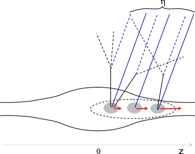
Figure 1: (Color online) Emission of particles from a boost-non-invariant fireball. The horizontal (vertical) axis indicates longitudinal coordinate $z$ (transverse coordinate $\rho$). Particles emitted with the same value of pseudorapidity $\eta$ originate from different regions of the fireball indicated by the gray blobs (they also are emitted at different times). The thermal conditions and flow (indicated by arrows) in these regions are different. The solid lines indicate tracks of primordial particles, while the dashed lines show products of resonance decays. The dashed ellipse indicates the relevant region for a give $\eta$, which spans about two units of the spatial rapidity $\alpha_{\parallel}$.

When the system is not boost invariant the above simplifications no longer hold. The situation is illustrated in Fig. 1. Particles detected at a given pseudorapidity $\eta$ (parallel lines in the figure) originate from different pieces of the fireball (gray blobs). Thermal conditions (temperature, chemical potentials, flow) change from piece to piece, which must be properly included. In addition, the effects of the longitudinal flow (indicated by arrows) must be incorporated, and the kinematics of resonance decays (dashed lines) becomes relevant. Although the resulting formalism for particle spectra remains conceptually simple and is based on the standard Cooper-Frye treatment, the calculation is no longer semi-analytic and a full-fledged simulation is necessary to accomplish the goal.

In the analysis of this paper we use THERMINATOR – the THERMal heavy IoN generATOR Kisiel et al. (2006a), to generate the Monte Carlo events in a suitably modified single-freeze-out model of Ref. Broniowski and Florkowski (2001). The extension to the boost-non-invariant case consists of two basic elements. The first one (geometric) is the choice of the shape of the freeze-out hypersurface $\Sigma$ and collective expansion. The other one incorporates the dependence of the thermal parameters on the position within the hypersurface $\Sigma$. Specifically, in our treatment the transverse size and the chemical potentials depend on the spatial rapidity $\alpha_{\parallel}=\mathrm{arctanh}(z/t)$, where $z$ and $t$ are the longitudinal and time coordinates on the freeze-out hypersurface. Although the boost-non-invariant model has quite a few parameters, as listed at the end of Sect. II, they can be fitted independently to various combinations of the data, leaving little freedom. For instance, the $\alpha_{\parallel}$ dependence of the baryon and strange chemical potentials is fixed with the ratios of protons to antiprotons and $K^{+}$ to $K^{-}$. The result in the range of the BRAHMS data is the expected growth of the baryon and strange chemical potentials with $|\alpha_{\parallel}|$. The value of the baryon chemical potential $\mu_{B}$ at $\alpha_{\parallel}\sim 3$, which is the relevant region for particles detected at the BRAHMS forward rapidity, $y\sim 3$, is about $200~{}{\rm GeV}$. This value is in the range of the values of the thermal fits for the highest SPS energy, thus we confirm the recent findings by Roehrich Roehrich (Florence, 3-6 July 2006) that the thermal conditions at RHIC at forward rapidities, $y\sim 3$, correspond to the SPS conditions at mid-rapidity. Details of our procedure of determining the dependence of thermal parameters on $\alpha_{\parallel}$ are explained in Sect. III. Our strategy, as usual, is to fix the features of the fireball with the well-measured spectra of particles: pions, kaons, protons and antiprotons. The strange chemical potential obtained from the fit to the $K^{+}/K^{-}$ ratio is such that the local strangeness density on the freeze-out hypersurface $\Sigma$ is compatible with zero. The experimental Bearden et al. (2003) rapidity spectra of net protons, $p-\bar{p}$, are reproduced qualitatively in the model, displaying the correct shape but overshooting the data at larger rapidities by about 50%. The chosen geometry of the fireball incorporates a decreasing transverse size as $|\alpha_{\parallel}|$ is increased, which simultaneously results in a decreasing transverse flow. This choice is verified in Sect. III by reproducing the spectra $d^{2}N/(2\pi p_{T}dp_{T}dy)$ at a fixed $y$ of pions and kaons at $\sqrt{s_{NN}}=200~{}\mathrm{GeV}$ from the BRAHMS collaboration Bearden et al. (2005). These transverse-momentum spectra exhibit slopes which become steeper with rapidity.

As a result of our study, we obtain the “topography” of the fireball, which can be the ground for other more detailed studies, discussed in the Conclusion.

II The single freeze-out model

The single-freeze-out model is described in detail in Refs. Broniowski and Florkowski (2001, 2002); Broniowski et al. (2002). Here we review the main assumptions and the formalism of describing the expansion and particle decays.

1. At a certain stage of evolution of the fireball the thermal equilibrium between hadrons is reached. Most probably, hadrons are “born” already in such an equilibrated state. The local particle phase-space densities have the form of the Fermi-Dirac or Bose-Einstein statistical distributions. The particles generated at freeze-out are termed primordial. For simplicity of the model we do not include the $\gamma$ non-equilibrium factors of Ref. Rafelski (1991) used in several recent analyses Torrieri and Rafelski (2004); Becattini et al. (2004); Cleymans et al. (2005).

2. The thermodynamic parameters are the freeze-out temperature $T$ and three chemical potentials: baryon, $\mu_{B}$, strange, $\mu_{S}$, and $\mu_{I_{3}}$, related to the third component of isospin. In a boost-non-invariant model the values of these parameters depend on the position within the freeze-out hypersurface $\Sigma$.

3. In the boost-non-invariant model the shape of the fireball is nontrivial in the longitudinal direction. In this paper we retain the azimuthal symmetry.

4. The velocity field of the collective expansion is chosen in the form of the Hubble flow Csorgo and Lorstad (1996), providing the longitudinal and transverse flow to the system. Again, in the boost-non-invariant model the functional form of the velocity field may depend on the longitudinal position.

5. The evolution after freeze-out includes decays of resonances which may proceed in cascades. All resonances from the Particle Data Tables Hagiwara et al. (2002) are incorporated.

6. Elastic rescattering among particles after the chemical freeze-out is ignored and the model may be viewed as an approximation to a more detailed evolution, taking into account different time scales for various hadronic processes (see Heinz (1999) and references therein).

The single freeze-out concept complies to the explosive scenario at RHIC Rafelski and Letessier (2000). Moreover, the approach reproduces very efficiently the particle abundances, the transverse-momentum spectra, including particles with strangeness Broniowski and Florkowski (2002), produces very reasonable results for the resonance production Broniowski et al. (2003a), the charge balance functions in rapidity Bozek et al. (2005), the elliptic flow Broniowski et al. (2003b), the HBT radii Kisiel et al. (2006b), and the transverse energy Prorok (2005, 2006a, 2006b). Recently with the help of RQMD Sorge et al. (1989) it was found (cf. Fig. 16 and 17 of Ref. Nonaka and Bass (2006)) that the elastic rescattering effects are not significant for the mid-rapidity $p_{T}$ spectra of pions. One can understand this as follows: resonance decays “cool” the spectra Broniowski and Florkowski (2001). As the result, the original $\sim 165~{}\mathrm{MeV}$ spectra from the chemical freeze-out look, after feeding from resonances, approximately as $\sim 130~{}\mathrm{MeV}$ spectra, which would be obtained at the the lower temperature of the thermal freeze-out. Thus elastic rescattering becomes innocuous. Certainly, more studies are desirable here, in particular an “afterburner” performing elastic rescattering could be run on top of our simulation. It would help to achieve a more accurate collision picture, with the elastic rescattering processes taken fully into account.

Popular choices of the freeze-out hypersurface and the collective velocity field are discussed in detail in Ref. Florkowski and Broniowski (2004). In this work we modify in a very simple way the original boost-invariant single-freeze-out model of Ref. Broniowski and Florkowski (2001, 2002); Broniowski et al. (2002) by making the transverse size of the fireball dependent on the spatial rapidity. We use the freeze-out hypersurface parameterized as

$$x^{\mu}=\left(\begin{array}[]{c}t\\ x\\ y\\ z\end{array}\right)=\left(\begin{array}[]{l}\tau\mathrm{cosh}\alpha_{\perp}\mathrm{cosh}\alpha_{\parallel}\\ \tau\mathrm{sinh}\alpha_{\perp}\cos\phi\\ \tau\mathrm{sinh}\alpha_{\perp}\sin\phi\\ \tau\mathrm{cosh}\alpha_{\perp}\mathrm{sinh}\alpha_{\parallel}\end{array}\right).$$ (10)

The parameter $\alpha_{\parallel}$ is the spatial rapidity, while $\alpha_{\perp}$ is related to the transverse radius as

$$\rho=\sqrt{x^{2}+y^{2}}=\tau\mathrm{sinh}\alpha_{\perp}.$$ (11)

The four-velocity field is chosen to follow the Hubble law

$$u^{\mu}=x^{\mu}/\tau.$$ (12)

We note that the longitudinal flow is $v_{z}=\hbox{tanh}\,\alpha_{\parallel}=z/t$ (as in the one-dimensional Bjorken model Bjorken (1983)), while the transverse flow (at $z=0$) has the form $v_{\rho}=\hbox{tanh}\,\alpha_{\perp}$.

The new element of the parameterization of this paper, which implements the departure from boost invariance, is the selection of boundaries for the fireball. In the boost invariant model $\rho$ was limited by the space-independent parameter $\rho_{\mathrm{max}}$, or $0\leq\alpha_{\perp}\leq\alpha_{\perp}^{\mathrm{max}}$. Now we take

$$0\leq\alpha_{\perp}\leq\alpha_{\perp}^{\mathrm{max}}(\alpha_{\parallel})\equiv\alpha_{\perp}^{\mathrm{max}}(0)\exp\left(-\frac{\alpha_{\parallel}^{2}}{2\Delta^{2}}\right).$$ (13)

The interpretation of this formula is clear: as we depart from the center by increasing $|\alpha_{\parallel}|$, we simultaneously reduce $\alpha_{\perp}$, or $\rho_{\mathrm{max}}$. The rate of this reduction is controlled by a new model parameter, $\Delta$. Since in our model the flow is linked to the position via Eq. (12), we also have less transverse flow as we increase $|\alpha_{\parallel}|$. This feature will show in the $p_{T}$ spectra presented in Sect. III. We may also use more conveniently the parameter

$$\rho_{\mathrm{max}}^{(0)}=\mathrm{sinh}\alpha_{\perp}^{\mathrm{max}}(0).$$ (14)

Thus the geometry and expansion of the fireball is described by three parameters: $\tau$, $\rho_{\mathrm{max}}^{(0)}$, and $\Delta$.

With the standard parameterization of the particle four-momentum in terms of rapidity $y$ and the transverse mass $m_{\perp}$,

$$p^{\mu}=\left(m_{\perp}\hbox{cosh}y,p_{\perp}\cos\varphi,p_{\perp}\sin\varphi,m_{\perp}\hbox{sinh}y\right),$$ (15)

we find with Eqs. (10) and (12)

$$p\cdot u=m_{\perp}\hbox{cosh}(\alpha_{\perp})\hbox{cosh}(\alpha_{\parallel}-y)-p_{\perp}\hbox{sinh}(\alpha_{\perp})\cos(\phi-\varphi),$$ (16)

and

$$d^{3}\Sigma\cdot p\!\! = \!\!d\alpha_{\parallel}d\phi\,\rho\,d\rho\times$$ (17)

$$\left[m_{\perp}\sqrt{\tau^{2}+\rho^{2}}\,\hbox{cosh}(\alpha_{\parallel}-y)-p_{\perp}\rho\cos(\phi-\varphi)\right]$$

$$= \tau^{3}d\alpha_{\parallel}d\phi\,\mathrm{sinh}\alpha_{\perp}\,d\alpha_{\perp}\,p\cdot u$$

where $d^{3}\Sigma^{\mu}$ is the volume element of the hypersurface. With the assumed azimuthal symmetry the Cooper-Frye Cooper and Frye (1974) formalism then yields the following expression for the momentum density of a given species of primordial particles:

$$\frac{d^{2}N}{2\pi p_{T}dp_{T}\,dy} = \tau^{3}\!\!\int_{-\infty}^{\infty}\!\!\!\!\!\!d\alpha_{\parallel}\int_{0}^{\alpha_{\perp}^{\mathrm{max}}(\alpha_{\parallel})}\!\!\!\!\!\!\!\!\!\!\!\!\!d\alpha_{\perp}\int_{0}^{2\pi}\!\!\!\!\!\!d\phi$$ (18)

$$\times p\cdot uf\left(\beta p\cdot u-\beta\mu(\alpha_{\parallel})\right),$$

$$f(z) = \frac{1}{(2\pi)^{3}}\frac{1}{\exp z\pm 1},$$

where $p\cdot u$ from Eq. (16) is taken at $\varphi=0$, $f(z)$ is the statistical distribution function (with $+$ for fermions and $-$ for bosons), $\beta=1/T$, and

$$\mu(\alpha_{\parallel})=B\mu_{B}(\alpha_{\parallel})+S\mu_{S}(\alpha_{\parallel})+I_{3}\mu_{I_{3}}(\alpha_{\parallel}),$$ (19)

with $B$, $S$, and $I_{3}$ denoting the baryon number, strangeness, and the third component of isospin of the particle. Thus we admit the dependence of chemical potentials on the spatial rapidity. This is of course necessary if we wish to describe in the framework of a statistical model the increasing density of net protons as we move from mid-rapidity towards the fragmentation region.

The temperature $T$ also in general depends on $\alpha_{\parallel}$. The best model-building strategy here would be to use the universal Cleymans-Redlich chemical freeze-out curve Cleymans and Redlich (1998) in the $\mu_{B}$-$T$ space (for a recent status see Ref. Becattini et al. (2004); Cleymans et al. (2006)). That way the functional dependence of $\mu_{B}$ on $\alpha_{\parallel}$ induces unambiguously the dependence of $T$ on $\alpha_{\parallel}$. In this work, however, we apply the model for not too large values of the rapidity, $|y|\leq 3.3$, and it will turn out that the obtained values for $\mu_{B}$ are less than $\sim 250~{}\mathrm{MeV}$. The universal freeze-out curve gives from $\mu_{B}=0$ to $\mu_{B}=250~{}\mathrm{MeV}$ a practically constant value of $T$. For instance, at SPS ($Pb+Pb$, $\sqrt{s_{NN}}=17~{}\mathrm{GeV}$) one has Michalec (2001) $T=164\mathrm{~{}MeV}$, $\mu_{B}=229\mathrm{~{}MeV}$, $\mu_{S}=54\mathrm{~{}MeV}$, and $\mu_{I_{3}}=-7\mathrm{~{}MeV}$, with the value of $T$ equal within errors to the RHIC value of 165 MeV. For this reason in the present analysis we fix the freeze-out temperature at a constant (independent of the spatial rapidity) value,

$$T=165~{}\mathrm{MeV}.$$ (20)

If modeling were made for larger values of the rapidity and/or lower collision energies, the dependence of $T$ on $\alpha_{\parallel}$ should be incorporated according to the prescription based on the universal freeze-out curve. Eventually, we expect that when the fragmentation region is approached, $T$ becomes very small and $\mu_{B}$ reaches the value of the order of 1 GeV.

Another qualitative argument for the approximate constancy of $T$ at moderate values of $|\alpha_{\parallel}|$ may be inferred directly from the BRAHMS data. From the measured rapidity spectra (cf. Fig. 5), obviously, the yields of pions and kaons decrease with $y$. Thus, one needs to decrease the size of the emitting source, decrease the freeze-out temperature, or both. The decrease of temperature affects more strongly the particles with larger masses, since the thermal factor is approximately $\exp(-\sqrt{m^{2}+{\mathchoice{\mbox{\boldmath$\displaystyle p$}}{\mbox{\boldmath$\textstyle p$}}{\mbox{\boldmath$\scriptstyle p$}}{\mbox{\boldmath$\scriptscriptstyle p$}}}^{2}}/T)$. Therefore, if we introduced variation of the temperature with the spatial rapidity, it would result in a faster drop with $y$ of the pion yields compared to the kaons. Certainly the data excludes this situation, since the ratio of $dN_{\pi}/dy$ to $dN_{K}/dy$ is within a few percent independent of $y$ in the BRAHMS rapidity coverage. Therefore we must keep $T$ constant (within a few percent), and the remaining possibility is the decrease of the source size with $|\alpha_{\parallel}|$. Resonance decays complicate the above qualitative argument, but with the help of a numerical simulation we confirm it. Another way of providing the drop of yields with rapidity is to incorporate the $\gamma$ non-equilibrium factors Rafelski (1991) dependent on $\alpha_{\parallel}$, which may dilute the system as $|\alpha_{\parallel}|$ increases. We do not explore this possibility here.

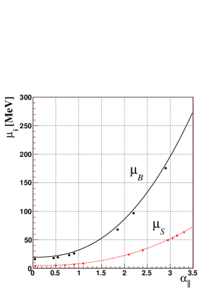
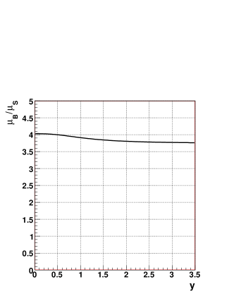
Figure 2: (Color online) Top: the model baryon and strange chemical potentials plotted as functions of the spatial rapidity. Parameters of Eq. (21) are obtained from the fit to the BRAHMS data Bearden et al. (2003, 2005). The points represent a naive calculation based of Eq. (23). Bottom: the ratio of the baryon to strange chemical potentials, $\mu_{B}/\mu_{S}$.

For convenience, we parameterize functionally the dependence of the chemical potentials at low values of $|\alpha_{\parallel}|$ as follows:

$$\mu_{i}(\alpha_{\parallel})=\mu_{i}(0)\left[1+A_{i}\alpha_{\parallel}^{2.4}\right],\;\;\;i=B,S,I_{3}.$$ (21)

The chosen power of 2.4 works somewhat better than 2. Of course, any convenient and sufficiently rich parametric form is admissible here, as it is fitted to the data (see Sect. III) and the introduced parameters effectively are not free. By “low” $|\alpha_{\parallel}|$ we mean the values relevant to the BRAHMS data, covering $|y|\leq 3.3$.

Formula (II) provides the spectra of the primordial particles. The following evolution of the system consists of free streaming, with resonances decaying into the daughter particles. We use THERMINATOR to perform the simulation. The code incorporates all the **** and *** resonances. Following the scheme of SHARE Torrieri et al. (2005) it excludes all * resonances, and practically all ** resonances listed in the Particle Data Tables Hagiwara et al. (2002). Each resonance decays at the time controlled by its lifetime, $1/\Gamma$. In the resonance’s rest frame the decay at time $t$ occurs with the probability density $\Gamma\exp(-\Gamma t)$. The two-body or three-body decay channels are incorporated and the values of the branching ratios are taken from the Particle Data Tables. Heavy resonances may of course decay in cascades.

Let us summarize the model parameters. We have the universal freezeout temperature $T$, three chemical potentials at mid-rapidity, $\mu_{B}(0)$, $\mu_{S}(0)$, $\mu_{I_{3}}(0)$, three parameters $A_{B}$, $A_{S}$, and $A_{I_{3}}$ of Eq. (21) describing the dependence of the chemical potentials on the spatial rapidity, and three geometry/expansion parameters: the proper time $\tau$, the transverse size at mid-rapidity, $\rho_{\mathrm{max}}^{(0)}$, and the parameter $\Delta$ controlling the spatial rapidity dependence of the transverse size. Except for $T$ taken to have the value (20) obtained in earlier thermal analyses of particle ratios Broniowski and Florkowski (2001), the remaining parameters are fitted to the BRAHMS data Bearden et al. (2003, 2005) for the double differential spectra $d^{2}N/(2\pi p_{T}dp_{T}dy)$.

III Results

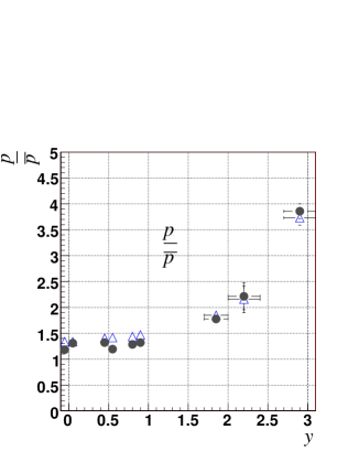
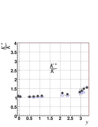
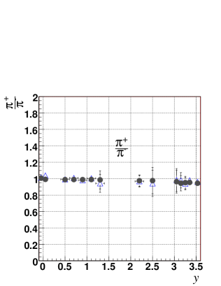
Figure 3: (Color online) Dependence of particle ratios on rapidity: top – $p/{\bar{p}}$, middle – $K^{+}/K^{-}$, bottom – $\pi^{+}/\pi^{-}$. The open triangles are the Brahms data Bearden et al. (2003, 2005), while the filled circles show the result of the model simulation with THERMINATOR. The model parameters are given in Eq. (25). The data for $p$ and $\bar{p}$ are not corrected for the feed-down from weak-decays Bearden et al. (2003).

We first describe our fitting strategy, which with many parameters present must be done with care. We wish to have a good starting point for the parameters describing the chemical potentials. Practice shows that to a very good approximation the statistical distributions are very well approximated by the Boltzmann factors. Then the integrand of Eq. (18) contains the factor $\exp[-\beta m_{\perp}\mathrm{cosh}(\alpha_{\perp})\mathrm{sinh}(\alpha_{\parallel}-y)+\beta\mu(\alpha_{\parallel})]$. Because of this the relevant integration range in $\alpha_{\parallel}$ is sharply peaked around $\alpha_{\parallel}\simeq y$ (the half-width is about one unit of $\alpha_{\parallel}$) and the chemical potentials entering the formula are taken approximately at $\mu_{i}(\alpha_{\parallel})\simeq\mu_{i}(y)$. Thus the factors $\exp[\beta\mu(y)]$ can be taken in front of the integration. If it were not for the resonance decays which modify the result (and are included in the full simulation) we would have to a good approximation the following relations:

$$\frac{p}{\bar{p}} \simeq \exp(2\beta\mu_{B}),$$

$$\frac{K^{+}}{K^{-}} \simeq \exp(2\beta\mu_{S}),\;\;\;\mathrm{(approximate~{}formulas)}$$

$$\frac{\pi^{+}}{\pi^{-}} \simeq \exp(2\beta\mu_{I_{3}}).$$ (22)

The symbols on the left-hand side denote the ratios of yields of the specified particles at a fixed $y$ and integrated over $p_{T}$. These are known form the data, thus we can invert

$$\mu_{B}(y)=\frac{1}{2}T\log(p/{\bar{p}}),\;\;\;\mathrm{(approximate~{}formula)}$$ (23)

and so on. With the help of this form we set the starting values of the parameters $\mu_{i}(0)$ and $A_{i}$, which are then iterated. The iteration proceeds as follows: for a given set of parameters we run the full THERMINATOR simulation, which generates events. We first optimize the baryon-number parameters $\mu_{B}(0)$ and $A_{B}$ with the help of the ratio of the $p$ and ${\bar{p}}$ rapidity spectra, then the strangeness parameters $\mu_{S}(0)$ and $A_{S}$ using the $K^{+}$ to $K^{-}$ ratio, then we go back again to the baryon parameters, etc., and loop until a fixed is reached. The isospin parameters $\mu_{I_{3}}(0)$ and $A_{I_{3}}$ are consistent with zero and thus irrelevant. The $\Delta$ parameter is fixed with the pion rapidity spectra $dN_{\pi^{\pm}}/dy$. The optimum value is

$$\Delta=3.33.$$ (24)

The result of our optimization for the chemical potentials is shown in Fig. 2. The optimum parameters are:

$$\!\!\!\!\!\!\!\!\mu_{B}(0)=19~{}{\rm MeV},\;\mu_{S}(0)=4.8~{}{\rm MeV},\;\mu_{I_{3}}(0)=-1~{}{\rm MeV},$$

$$\!\!\!A_{B}=0.65,\;A_{S}=0.70,\;A_{I_{3}}=0.$$ (25)

We observe the expected behavior for the baryon chemical potential, which increases with $|\alpha_{\parallel}|$. The value at the origin is 19 MeV, somewhat lower than the earlier mid-rapidity fits made in boost-invariant models in Refs. Broniowski and Florkowski (2001); Braun-Munzinger et al. (2001), yielding 26 MeV. The lower value in our case is well understood. The previous mid-rapidity fits include the data in the range $|y|\leq 1$. This range collects the particles emitted from the fireball at $|\alpha_{\parallel}|\leq 2$, hence the value of $\mu_{B}$ in the previous mid-rapidity fits is an average of our $\mu_{B}(\alpha_{\parallel})$ over the range, approximately, $|\alpha_{\parallel}|\leq 2$, with some weight proportional to the particle abundance. This qualitatively explains the effect of a lower value of our $\mu_{B}(0)$ than in the boost-invariant models. A similar effect occurs for $\mu_{S}$. We do not incorporate corrections for the feed-down from weak decays (em i.e. all decays are included), since this is the policy of Ref. Bearden et al. (2003) for the treatment of $p$ and $\bar{p}$.

We note that at $\alpha_{\parallel}=3$ the value of $\mu_{B}$ is 200 MeV, more than 10 times larger than at the origin. This value is comparable to the highest-energy SPS fit ($\sqrt{s_{NN}}=17~{}\mathrm{GeV}$), where $\mu_{B}\simeq 230~{}\mathrm{MeV}$. The behavior of the strange chemical potential is qualitatively similar. It also increases with $|\alpha_{\parallel}|$, growing form 5 MeV at the origin to 50 MeV at $\alpha_{\parallel}=3$. The ratio $\mu_{B}(\alpha_{\parallel})/\mu_{S}(\alpha_{\parallel})$ is very close to a constant, $\simeq 4-3.5$, as can be seen in the bottom panel of Fig. 2.

The points in the top panel of Fig. 2 show the result of the naive calculation of Eq. (22,23). We note that these points are very close (in particular for the strangeness case) to the result of the full-fledged fit of our model. This is of practical significance, since the application of Eq. (22,23) involves no effort, while the model calculation incorporating resonance decays, flow, etc., is costly.

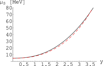
Figure 4: (Color online) Comparison of the strange chemical potential obtained from the fit to the data (solid line) and from the condition of zero local strangeness density, $\rho_{S}=0$ (dashed line).

There is another important point. In thermal models one may obtain the local value of the strange chemical potential, $\mu_{S}$, at a given $\mu_{B}$ with the condition of the vanishing strangeness density, $\rho_{S}=0$. The result is shown in Fig. 4, where we compare the strange chemical potential obtained from the fit to the data (solid line) and from the condition of zero local strangeness density at a given $\mu_{B}(\alpha_{\parallel})$. The two curves turn out to be virtually the same. This shows that the net strangeness density in our fireball is, within uncertainties of parameters, compatible with 0. This is not obvious from the outset, as the condition of zero strangeness density is not assumed in our fitting procedure. Although this feature is natural in particle production mechanisms, in principle only the total strangeness, integrated over the whole fireball, must be initially zero. Variation of the strangeness density with $\alpha_{\parallel}$ is admissible, but turns out not to occur.

Figure 3 shows the quality of our fit for the parameters of chemical potentials, Eq.(25). We show the measured ratios of $p/{\bar{p}}$, $K^{+}/K^{-}$, and $\pi^{+}/\pi^{-}$ as a function of rapidity $y$ Bearden et al. (2003, 2005) and the results of fit made with help of the simulation with THERMINATOR. We note a very reasonable agreement. The error bars on the model points are statistical errors due to the finite size of the sample (we use 2500 simulated events in this plot). The flat character of the $\pi^{+}/\pi^{-}$ ratio indicates that the value of the isospin chemical potential is consistent with zero at all spatial rapidity values.

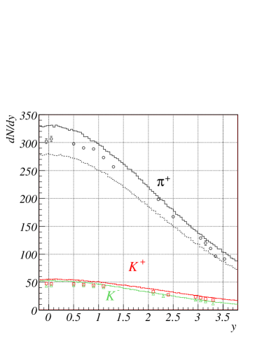
Figure 5: (Color online) Rapidity spectra of $\pi^{+}$, $K^{+}$, and $K^{-}$. The data points come from the BRAHMS collaboration Bearden et al. (2003, 2005) (circles - $\pi^{+}$, squares - $K^{+}$, triangles - $K^{-}$), while the histogram lines show the result of the model simulation with THERMINATOR. For $\pi^{+}$ the solid (dashed) line corresponds to the full feeding (no feeding) from the weak hyperon decays. The model parameters are from Eq. (25). The experimental pion yields are corrected for weak decays as described in Bearden et al. (2005).

In Fig. 5 we show the comparison of obtained rapidity spectra of $\pi^{+}$, $K^{+}$, and $K^{-}$ to the experimental data. The experimental yields for the pions are corrected for the feed-down from the weak decays as described in Ref. Bearden et al. (2005). For that reason for the case of $\pi^{+}$ we give the model predictions with the full feeding from the weak decays (solid line) and with no feeding from the weak decays at all (dashed line). We note a quite good quantitative agreement, with the data falling between the two extreme cases. We recall that the behavior on rapidity of $dN/dy$ is controlled by the $\Delta$ parameter of Eq. (13). The spectra of $\pi^{-}$ are not shown, since they are practically equal to the case of $\pi^{+}$. The spectra of $K^{+}$ and $K^{-}$ are also quite well reproduced.

Figure 6 displays the rapidity spectra of protons and antiprotons, as well as their difference $p-\bar{p}$, i.e. the net protons. Since the $p$ and $\bar{p}$ data carry no feed-down corrections for weak decays Bearden et al. (2003), one should compare the solid lines to the data. The shape of the $p$ and $\bar{p}$ spectra is properly reproduced, but the model overshoots the data by about 50%. This feature occurs at all rapidities, also at mid-rapidity. The mismatch could be improved by decreasing $T$ by a few percent and redoing the whole analysis, but we do not take the effort here, holding to the value (20) obtained from global fits to all RHIC data for the particle yields at midrapidity. We provide, however, the results of the model calculation with no feeding from the hyperon decays, since it provides some measure of the systematic uncertainties in determining the proton and antiproton yields.

Quite remarkably, the qualitative growing of the net-proton spectrum with $y$ is obtained. This has a simple explanation on the ground of statistical models, since approximately $p-\bar{p}\sim{\rm sinh}(\mu_{B}(y)/T)$. Thus at RHIC the proton and antiproton spectra may be qualitatively explained solely on the ground of the statistical approach.

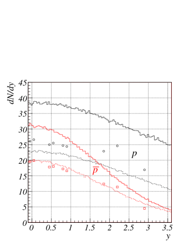
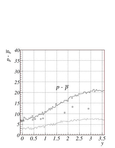
Figure 6: (Color online) Top: the rapidity spectra of $p$ and $\bar{p}$. Bottom: spectrum of net protons, $p-\bar{p}$. The data points come from the BRAHMS collaboration Bearden et al. (2003, 2005), while the solid (dashed) histogram lines show the result of the model simulation with THERMINATOR with full feeding (no feeding) from the weak hyperon decays. Data points should be compared to the model with full feeding (solid lines). The model parameters are from Eq. (25).

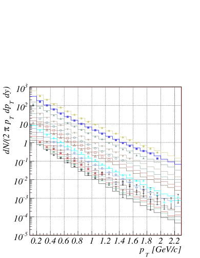
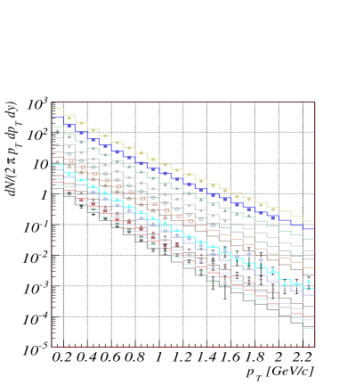
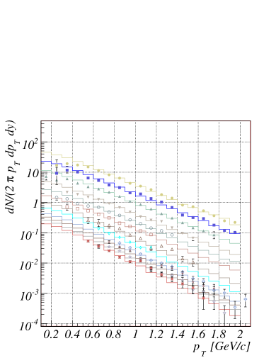
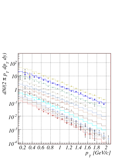
Figure 7: (Color online) The $p_{T}$-spectra of $\pi^{+}$ (top left), $\pi^{-}$ (top right), $K^{+}$ (bottom left), and $K^{-}$ (bottom right) in the subsequent BRAHMS rapidity bins, see the text for details. The data points come from Ref. Bearden et al. (2005), while the histogram lines show the result of the model simulation with THERMINATOR.

Figure 7 shows the $p_{T}$-spectra at subsequent rapidity bins of the BRAHMS experiment. From top to bottom we have for pions $y\in[-0.1,0.0]$, $[0.0,0.1]$,$[0.4,0.6]$, $[0.6,0.8]$, $[0.8,1.0]$, $[1.0,1.2]$, $[1.2,1.4]$, $[2.1,2.3]$, $[2.4,2.6]$, $[3.0,3.1]$, $[3.1,3.2]$, $[3.2,3.3]$, $[3.3,3.4]$, $[3.4,3.66],$ and for kaons $y\in[-0.1,0.0]$, $[0.0,0.1]$,$[0.4,0.6]$, $[0.6,0.8]$, $[0.8,1.0]$, $[1.0,1.2]$, $[2.0,2.2]$, $[2.3,2.5]$, $[2.9,3.0]$, $[3.0,3.1]$, $[3.1,3.2]$, and $[3.2,3.4]$. Each lower curve is subsequently divided by the factor of 2 in order to avoid overlapping. The solid lines show the model calculation with optimum parameters (25). We note that the basic features of the experiment are reproduced, with the slope increasing with $y$. This can be explained with a lower transverse flow at larger $y$, as enforced by the parameterization (13). The quality of the agreement is similar in all rapidity bins. In Fig. 8 we give the similar study for the protons and antiprotons. The data points come from the BRAHMS collaboration Bearden et al. (2003) and contain no weak-decay corrections, hence the solid lines should be compared to the data. Nevertheless, as in Fig. 6, we also present the calculation with feed-down from the weak decays switched off, as it provides a measure of systematic uncertainties. It should also be kept in mind that these uncertainties are quite large for the $p_{T}$-spectra of $p$ and $\bar{p}$, as can be inferred from the comparison of results of various experimental collaborations at RHIC (cf. for instance Fig. 12 of Ref. Ullrich (2003)).

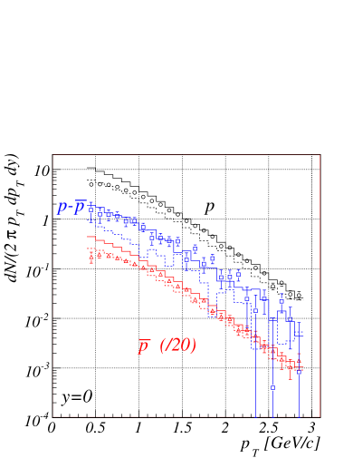
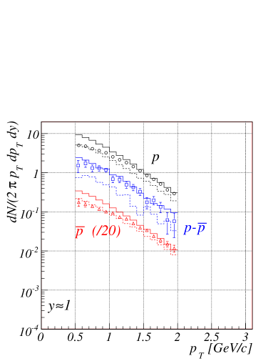
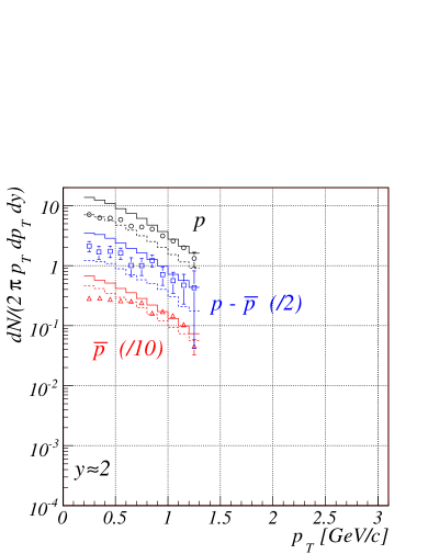
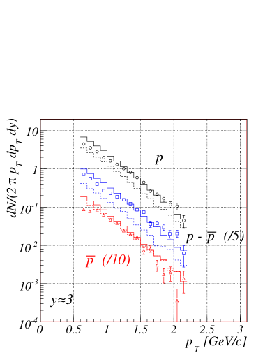
Figure 8: (Color online) The proton, antiproton, and net-proton transverse momentum spectra at $y\simeq 0,1,2,3$. The antiproton spectra and the net-proton spectra at $y\simeq 3$ have been divided by $10$. The data points come from the BRAHMS collaboration Bearden et al. (2003) and contain no weak-decay corrections. Solid (dashed) histogram lines show the result of the model simulation with full feeding (no feeding) from the weak hyperon decays. Solid lines should be compared to the data.

At this point we have accomplished the goal of fixing the “fireball topography”: we have the geometry/flow as well as thermal parameters dependent on the variable $\alpha_{\parallel}$. Next, we may proceed as in the case of the boost-invariant model used at mid-rapidity, and compute many observables in addition to those already used up to fix the model parameters. These observables include one-body observables, such as spectra of various particles, including hyperons, mesonic resonances, etc., as well as two-body observables related to correlations: HBT radii, balance functions in rapidity, or event-by-event fluctuations. Here we only present a sample prediction for rapidity spectra of hyperons, shown in Fig. 9.

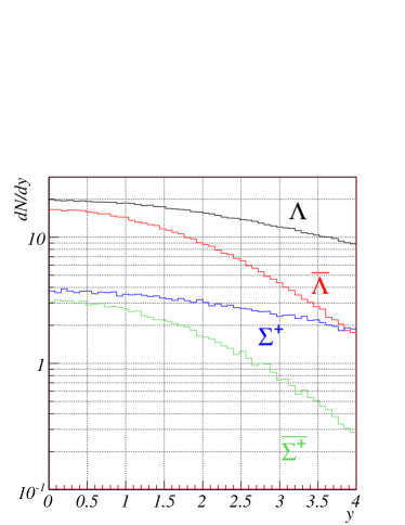
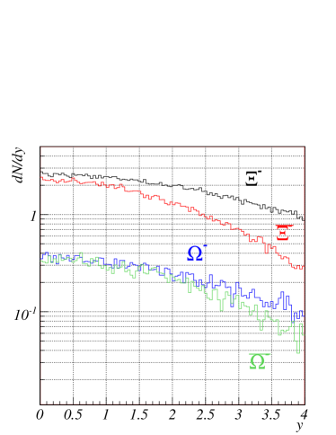
Figure 9: (Color online) The model predictions for the rapidity spectra of hyperons. Top panel, curves from top to bottom: $\Lambda$, $\bar{\Lambda}$, $\Sigma^{+}$, and $\bar{\Sigma}^{+}$. Bottom panel, curves from top to bottom: $\Xi^{-}$, $\bar{\Xi}^{-}$, $\Omega$, and $\bar{\Omega}$. The model parameters as in Fig. 3.

An interesting feature is the very small splitting of $\Omega$ and $\bar{\Omega}$, which results from the fact that $\mu_{B}-3\mu_{S}\simeq 0$, cf. Fig. 2.

IV Conclusion

The paper contains results of the single-freeze-out thermal model for rapidity-dependent spectra in relativistic heavy-ion collisions. We have used THERMINATOR to run the simulations and the BRAHMS data for $\sqrt{s_{NN}}=200~{}\mathrm{GeV}$ $Au+Au$ collisions to fix the model parameters. Such a simulation is necessary when the system is not boost-invariant. It allows for an exact incorporation of the space-time dependence of thermal parameters, precise inclusion of resonance decays, as well as incorporation of experimental cuts. The extension of the original boost-invariant single-freeze-out model includes a modification of the shape of the fireball, which here becomes narrower as the magnitude of the spatial rapidity $\alpha_{\parallel}$ increases, as well as admits the dependence of the thermal parameters on $\alpha_{\parallel}$. As a result of a fit to the BRAHMS data we have obtained the dependence of the freeze-out chemical potentials on $\alpha_{\parallel}$. The freeze-out temperature is taken constant in the considered range of rapidities. With this extension we are able to properly describe the double $d^{2}N/(2\pi p_{T}dp_{T}dy)$ spectra from the experiment. We also make predictions for other particles, in particular for hyperons.

A code incorporating the elastic collisions neglected in the single-freeze-out approach could be used as an “afterburner” starting from our freeze-out condition. That way a more accurate collision picture could be achieved. As we have already mentioned, a recent study of Ref. Nonaka and Bass (2006) revealed that for the mid-rapidity $p_{T}$-spectra the elastic rescattering is not very important.

Certainly, the scheme of this paper can be used for other collisions where departures from the boost invariance are significant, in particular for the rich SPS data. As we have said, the modeling involves the choice of the parameterization for the shape of the fireball and the velocity field of flow, where in fact we have quite a lot of freedom, as well as the dependence of the thermal parameters at freeze-out on the space-time position. Accurate data for numerous observables as functions of the rapidity, not only abundances and spectra but also the correlation data (HBT radii, balance functions), would greatly help to constrain the freedom and acquire insight into the space-time evolution picture of boost-non-invariant systems formed in relativistic heavy-ion collisions. Most importantly, the knowledge of the dependence of $R_{\rm side}$ on $y$ would put constraints on the shape of the fireball.

Here are the main results of the paper:

1. Naive extraction of the baryon and strange chemical potentials from ratios of $p/\bar{p}$ and $K^{+}/K^{-}$ works surprisingly well, as shown in the comparison to the full calculation in Fig. 2.

2. The baryon and strange chemical potentials grow with $\alpha_{\perp}$, reaching at $y\sim 3$ values close to those of the highest SPS energies of $\sqrt{s_{NN}}=17~{}{\rm GeV}$. This agrees with the recent conclusions of Roehrich Roehrich (Florence, 3-6 July 2006).

3. At mid-rapidity the values of the chemical potentials are even lower than derived from the previous thermal fits to the data for $|y|\leq 1$, with our values taking $\mu_{B}(0)=19~{}{\rm MeV}$ and $\mu_{S}(0)=5~{}{\rm MeV}$. The reason for this effect is that the particle with $|y|\leq 1$ originate from a region $|\alpha_{\parallel}|\leq 2$, and on the average the effective values of chemical potentials are larger compared to the values at the very origin (cf. Fig. 2).

4. The local strangeness density of the fireball is compatible with zero at all values of $\alpha_{\parallel}$. Although this feature is natural in particle production mechanisms, here it has been obtained independently just from fitting the chemical potentials to data.

5. The ratio of the baryon to strange chemical potentials varies very weakly with rapidity, ranging from $\sim 4$ at midrapidity to $\sim 3.5$ at larger rapidities.

6. The $d^{2}N/(2\pi p_{\perp}dp_{\perp}dy)$ spectra of pions and kaons are well reproduced, supporting our hypothesis for the shape of the fireball in the longitudinal direction.

7. The rapidity shape of the spectra of protons and antiprotons measured by BRAHMS Bearden et al. (2003) is described properly, while the model predict too large normalization, overproducing these particles by about 50%. This suggests a lower value of $T$ by a few percent, or presence of non-equilibrium factors. We also note that the feature of an increasing yield of the net protons with rapidity is obtained naturally, explaining the shape of the rapidity dependence on purely statistical grounds.