TUM-T39-06-13

The electromagnetic Nucleon to Delta transition in Chiral Effective Field Theory

Tobias A. Gail and Thomas R. Hemmert,

Theoretische Physik T39, Physik Department
TU-München, D-85747 Garching, Germany

We present a calculation of the three complex form factors parametrizing the nucleon to $\Delta$ transition matrix element in the framework of chiral effective field theory with explicit $\Delta$ degrees of freedom. The interplay between short and long range physics is discussed and estimates for systematic uncertainties due to higher order effect are given.

1 Introduction

In this talk we discuss the findings of reference [1], where the low energy behaviour of the nucleon to $\Delta$ electromagnetic transition ($N(p_{N})+\gamma^{*}(q)\rightarrow\Delta(p_{\Delta})$) was analyzed in the framework of chiral effective field theory. We give an overview of the theoretical tools which are utilized in such an analysis in the next section and discuss the results in the third paragraph.
Demanding Lorentz covariance, gauge invariance and parity conservation the matrix element of a vector $I\left(J^{P}\right)=\frac{3}{2}\left(\frac{3}{2}^{+}\right)$ to $\frac{1}{2}\left(\frac{1}{2}^{+}\right)$ transition (like $N\gamma^{*}\rightarrow\Delta$) can be parametrized in terms of three form factors, i.e. complex valued functions of the momentum transfer squared. For our calculation we follow the conventions of ref.[2] and choose the definition:

$$i\mathcal{M}_{\Delta\rightarrow N\gamma} = \sqrt{\frac{2}{3}}\,\frac{e}{2M_{N}}\bar{u}(p_{N})\gamma_{5}\bigg{[}G_{1}(q^{2})(\not\!q\epsilon_{\mu}-\not\!\epsilon q_{\mu})+\frac{G_{2}(q^{2})}{2M_{N}}(p_{N}\cdot\epsilon q_{\mu}-p_{N}\cdot q\epsilon_{\mu})$$ (1)

$$+\frac{G_{3}(q^{2})}{2\Delta}(q\cdot\epsilon q_{\mu}-q^{2}\epsilon_{\mu})\bigg{]}u^{\mu}_{\Delta}(p_{\Delta}).$$

Here $e$ denotes the charge of the electron, $M_{N}$ is the mass of a nucleon and $\Delta=M_{\Delta}-M_{N}$ the $\Delta$-nucleon mass splitting, $p_{N/\Delta}^{\mu}$ denotes the relativistic four-momentum of the outgoing nucleon/incoming $\Delta$ and $(q^{\mu}$, $\epsilon^{\mu})$ are the momentum and polarization vectors of the outgoing photon, respectively. From the point of view of chiral effective field theory the signatures of chiral dynamics in the $N\Delta$-transition are particularly transparent in the $G_{i}(q^{2}),\,i=1,2,3$ basis, which serves as the analogue of the Dirac- and Pauli-form factor basis in the vector current of a nucleon. However, most experiments and most model calculations refer to the multipole basis of the general $N\Delta$-transition current, i.e. the magnetic dipole $\mathcal{G}_{M}^{*}(Q^{2})$, electric quadrupole $\mathcal{G}_{E}^{*}(Q^{2})$ and Coulomb quadrupole $\mathcal{G}_{C}^{*}(Q^{2})$ form factor defined by Jones and Scadron [3]. Phenomenological information about the electromagnetic nucleon to $\Delta$ transition is gained in the process $e\,p\rightarrow e^{\prime}\,N\pi$ in the region of the $\Delta$-resonance (e.g. see ref.[4] and references given therein), which has access to a lot more hadron structure properties than just the $N\Delta$-transition current of eq.(1). However, we compare our results to experimental data assuming the approximate relations

$$\textnormal{EMR}(q^{2}) \equiv Re\left[\frac{E_{1+}^{I=3/2}(W_{res},q^{2})}{M_{1+}^{I=3/2}(W_{res},q^{2})}\right]\approx-\textnormal{Re}\left[\frac{\mathcal{G}_{E}^{*}(q^{2})}{\mathcal{G}_{M}^{*}(q^{2})}\right],$$ (2)

$$\textnormal{CMR}(q^{2}) \equiv Re\left[\frac{S_{1+}^{I=3/2}(W_{res},q^{2})}{M_{1+}^{I=3/2}(W_{res},q^{2})}\right]\approx$$ (3)

$$-\frac{\sqrt{((M_{\Delta}+M_{N})^{2}-q^{2})((M_{\Delta}-M_{N})^{2}-q^{2})}}{4M_{\Delta}^{2}}\textnormal{Re}\left[\frac{\mathcal{G}_{C}^{*}(q^{2})}{\mathcal{G}_{M}^{*}(q^{2})}\right].$$

Concerning the resonance pole contributions alone, the right hand side of the above equations represents the ratios at the T-matrix pole $M_{\Delta}=(1210-i\,50)$MeV [5]. In this work we assume that the form factor ratios are approximately equal to the outcome of the various data analyses of the electroproduction multipoles $M_{1+}^{I=\frac{3}{2}}$, $E_{1+}^{I=\frac{3}{2}}$ and $S_{1+}^{I=\frac{3}{2}}$. Ultimately the validity of this (approximate) connection between the pion-electroproduction multipoles and the $N\Delta$-transition form factors has to be checked in a full theoretical calculation.

2 Theoretical Framework

In this section we briefly introduce the theoretical tools necessary to calculate the $N\Delta$-matrix element eq.(1) at low energies. In reactions with small momentum transfer (typically $Q^{2}=-q^{2}\leq 0.2$GeV²) the nucleon can - due to a separation of scales (the pion is much lighter than the next heavier hadron) - clearly be divided into a long-ranging pion cloud and a small nucleon core. Chiral Effective Field Theory in the baryon sector (ChPT, for a classic paper see [6]) provides a systematic framework for the calculation of pion cloud dynamics and at the same time also encodes short range physics via local operators of (theoretically) undetermined strength. A formulation of ChPT suitable for the calculation of the $N\Delta$-transition is the “small scale expansion” (SSE) [7], which includes explicit $\Delta$ degrees of freedom and provides an expansion scheme for the chiral Lagrangean. This framework contains three light (the momentum transfer $|Q|$, the pion mass $m_{\pi}$ and the $\Delta$-nucleon mass splitting $\Delta$) and two heavy (the nucleon mass $M_{N}$ and the scale of chiral symmetry breaking $4\pi F_{\pi}$, where $F_{\pi}$ is the pion decay constant) scales and each ratio of a light to a heavy scale is counted as a small parameter of the same order: $\epsilon\in\{\frac{|Q|}{4\pi F_{\pi}},\frac{m_{\pi}}{4\pi F_{\pi}},\frac{\Delta}{4\pi F_{\pi}},\frac{|Q|}{M_{N}},\frac{m_{\pi}}{M_{N}},\frac{\Delta}{M_{N}}\}$.
The Lagrangean containing all terms necessary for a leading one loop order calculation (i.e. order $\epsilon^{3}$) reads [2, 7]:

$$\mathcal{L}_{SSE} = \mathcal{L}_{\pi\pi}^{(2)}+\mathcal{L}_{\pi N}^{(1)}+\mathcal{L}_{\pi\Delta}^{(1)}+\mathcal{L}_{\pi N\Delta}^{(1)}+\mathcal{L}_{\gamma N\Delta}^{(2)}+\mathcal{L}_{\gamma N\Delta}^{(3)}.$$ (4)

At leading order $\mathcal{L}_{\pi\pi}^{(2)}$ encodes the pion dynamics, while $\mathcal{L}_{\pi N}^{(1)}$ and $\mathcal{L}_{\pi\Delta}^{(1)}$ describe the pion-nucleon and the pion-$\Delta$ system respectively and $\mathcal{L}_{\pi N\Delta}^{(1)}$ contains the pion-nucleon-$\Delta$ coupling. These parts of the Lagrangean form the input (i.e. vertizes and propagators) for the leading one loop calculation. All Feynman diagrams of a photon field coupling to the $\pi N\Delta$ system contributing at order $\epsilon^{3}$ in the SSE scheme are shown in figure 1.
To the order we are working, the Lagrangeans $\mathcal{L}_{\gamma N\Delta}^{(2)}$ and $\mathcal{L}_{\gamma N\Delta}^{(3)}$ contribute only to the values of $G_{1}(0)$ and $G_{2}(0)$ at zero momentum transfer through local operators (represented by diagram (a) in figure 1). The strength of these operators is undetermined in the effective field theory approach and will be extracted from phenomenology in the next section. Our analysis [1] has shown, that the local operator which gives the contributions from the nucleon core to the form factor $G_{2}(Q^{2})$ a finite spacial extension (i.e. a contribution to the radius of this form factor which formally is of higher order) is underestimated by the strict counting rules and its inclusion extends the $Q^{2}$-range of applicability of the leading one loop calculation significantly. The dependence of the quantities $\mathcal{G}_{M}^{*}(Q^{2})$, EMR$(Q^{2})$ and CMR$(Q^{2})$ on the form factors $G_{1}(Q^{2})$, $G_{2}(Q^{2})$ and $G_{3}(Q^{2})$ is such, that this radius contribution only has a very small impact in the magnetic dipole form factor (which is highly dominated by $G_{1}(Q^{2})$), but has decisive influence in the quadrupole moments. Altogether we consider short range contributions to the static limit ($q^{2}=0$) of $G_{1}$ and $G_{2}$ and the radius of $G_{2}$ in our calculation which thus contains three free parameters. All coupling constants contained in the other parts of the Lagrangean are extracted from other observables.
Besides the analysis presented here the authors of reference [8] also performed an effective field theory calculation of the $N\Delta$-transition at leading one loop level. Let us briefly point out the differences between both ChPT calculations:

1. In reference [8] a different expansion scheme, namely the $\delta$-scheme [9] has been applied to introduce a hierarchy of terms. In this scheme not all ratios of a small to a large scale are counted as a small parameter of the same order – as it is done in the $\epsilon$-counting discussed above – but the small parameters are: $\delta^{2}\in\{\frac{\Delta^{2}}{(4\pi F_{\pi})^{2}},\frac{m_{\pi}}{4\pi F_{\pi}},\frac{|Q|^{n}}{(4\pi F_{\pi})^{n}}\}$. Thus the pion mass $m_{\pi}$ is counted to be of the order of the $\Delta$-nucleon mass-splitting squared. The order $n$ of the momentum transfer then depends on its typical size in the particular process: if $|Q|\approx m_{\pi}\Rightarrow n=2$ and if $|Q|\approx\Delta\Rightarrow n=1$. The different counting leads to a different estimate of the relevance (i.e. inclusion or omission at a certain order) of the Feynman diagrams contributing to the $N$ to $\Delta$ matrix element between the SSE and the $\delta$-expansion. Diagram (b) of figure 1, for instance, provides important structures for our result, while it is neglected in the $\delta$-counting approach at leading one loop level.

2. While we performed a non-relativistic expansion of the Lagrangean (i.e. not only considered the chiral symmetry breaking scale $4\pi F_{\pi}$ but also the nucleon mass $M_{N}$ as a large scale) reference [8] gives a covariant calculation (i.e. a resummation of all terms which are suppressed by any power of the nucleon mass at a certain order of the chiral symmetry breaking scale). The results show that the inclusion of all terms which are suppressed by inverse powers of the nucleon mass cancels out important parts of the curvature in the $Q^{2}$-dependence of the resulting form factors. The same effect has already been observed in the vector current of the nucleon [10, 11]. On the other hand the additional string of $\frac{m_{\pi}}{M_{N}}$-terms provides enough quark mass dependent structures to qualitatively describe their quark mass dependence up to currently available lattice data [12].

3. Each of the two studies includes short range physics in a different manner: In [1] we took into account the accordant contributions to $G_{1}(0)$ and $G_{2}(0)$ arising from the chiral Lagrangean and furthermore found short range physics to play an important role in the radius of the $G_{2}$ form factor. The authors of reference [8] deal with three structurally different free parameters: the coupling constants characterizing the magnetic dipole and the electric- and Coulomb quadrupole transitions. Furthermore, they effectively include vector-meson exchange by giving the magnetic dipole coupling a dipole-shape $Q^{2}$-dependence.
   Finally the extraction of the free parameters from different experimental data leads to further differences between the numerical results of both calculations.

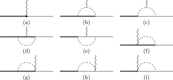
Figure 1: The diagrams contributing to the $\Delta\rightarrow N\gamma$ transition at leading-one-loop order in the SSE formalism [2]. The single solid lines represent nucleon-,the double lines $\Delta$-propagation. The dashed lines symbolize intermediate pion fields and the wiggly lines stand for the outgoing photon.

3 Discussion of the Results

The analytic expressions of the transition form factors resulting from a calculation in the SSE framework up to order $\epsilon^{3}$ can be found in reference [1]. In this section we give a brief overview of the findings presented there and discuss the size of the errors which arise as a consequence when neglecting higher order effects.
The three free parameters contained in our calculation are extracted from experimental data for the magnetic dipole form factor $\mathcal{G}_{M}^{*}(Q^{2})$ at $Q^{2}<0.2$GeV² and the value of EMR at the real photon point $Q^{2}=0$. Having fixed the low energy constants we arrive at the numerical values given in Table 1, where the real and imaginary parts of the static limit values and the radii defined through

$$G_{i}(Q^{2}) = \textnormal{Re}[G_{i}(0)]\left[1-\frac{1}{6}r_{i,\textnormal{Re}}^{2}Q^{2}+...\right]+i\,\textnormal{Im}[G_{i}(0)]\left[1-\frac{1}{6}r_{i,\textnormal{Im}}^{2}Q^{2}+...\right]$$ (5)

are shown for both sets of form factors discussed in this work. It is worth mentioning that the real parts of the radii of both the electric and the Coulomb $N\Delta$-transition form factors are negative!

	$\textnormal{Re}[G_{i}(0)]$	$r_{i,\textnormal{Re}}^{2}$ [fm2]	$\textnormal{Im}[G_{i}(0)]$	$r_{i,\textnormal{Im}}^{2}$ [fm2]	$\left|G_{i}(0)\right|$	$r_{i,\textnormal{Abs}}^{2}$ [fm2]
$G_{1}$	4.95	0.679	0.216	3.20	4.96	0.678
$G_{2}$	5.85	3.15	-10.0	1.28	11.6	1.73
$G_{3}$	-2.28	3.39	2.01	-2.26	3.04	0.907
$\mathcal{G}_{M}^{*}$	2.98	0.627	-0.377	1.36	3.00	0.630
$\mathcal{G}_{E}^{*}$	0.0441	-0.836	-0.249	0.422	0.253	0.388
$\mathcal{G}_{C}^{*}$	1.10	-0.729	-1.68	1.90	2.01	1.10

Table 1: The values of the form factors defined in eq.(1) and the Jones-Scadron form factors [3] at $Q^{2}=0$ and their radii [1].

While all imaginary parts occurring in our analysis are solely generated by pion cloud effects, the numerical values for the real parts result from an interplay between short and long range physics. Separating their contributions to the static limit one finds:

$$\textnormal{Re}[\mathcal{G}_{M}^{*}(0)]|_{\lambda=1\,\textnormal{GeV}} = \left.-1.06\right|_{pc}+\left.4.04\right|_{sd},$$ (6)

$$\textnormal{Re}[\mathcal{G}_{E}^{*}(0)]|_{\lambda=1\,\textnormal{GeV}} = \left.0.155\right|_{pc}-\left.0.110\right|_{sd},$$ (7)

$$\textnormal{Re}[\mathcal{G}_{C}^{*}(0)]|_{\lambda=1\,\textnormal{GeV}} = \left.1.47\right|_{pc}-\left.0.365\right|_{sd},$$ (8)

where “ sd” marks contributions from short distance physics while “pc” labels pion cloud effects. The physical interpretation of this is that the pion cloud strongly shields the characteristic of the nucleon core. Qualitatively the same statement can be made about the form factor basis defined in eq.(1). An analogous effect has e.g. already been observed in the anomalous magnetic moment of the nucleon [10]. The situation is somewhat different for the radii: While we find that approximately 22% of the squared radius of $G_{2}$ originate from short range physics [1], the translation into the Jones-Scadron basis drastically amplifies this contribution to the radii of the quadrupole form factors :

$$r_{M,\textnormal{Re}}^{2} = \left(\left.0.650\right|_{\textnormal{pc}}-\left.0.023\right|_{\textnormal{sd}}\right)\textnormal{fm}^{2},$$ (9)

$$r_{E,\textnormal{Re}}^{2} = \left(\left.1.31\right|_{\textnormal{pc}}-\left.2.15\right|_{\textnormal{sd}}\right)\textnormal{fm}^{2},$$ (10)

$$r_{C,\textnormal{Re}}^{2} = \left(\left.-0.019\right|_{\textnormal{pc}}-\left.0.710\right|_{\textnormal{sd}}\right)\textnormal{fm}^{2}.$$ (11)

All parts marked as short distance contributions in eqs. (9)-(11) exclusively arise from the local operator contributing to $r_{2,\textnormal{Re}}^{2}$. From this observation one can see that the $G_{i}$ basis is clearly preferred for the discussion of chiral signatures in the $N\Delta$-transition as there are fewer kinematical cancellations between large numbers in this basis. At the order of our calculation all effects beyond the linear $Q^{2}$-dependence of the form factors and hence the rich structures seen in figures 2-4 exclusively originate from pion cloud dynamics.
In addition to these results ChEFT provides us with the knowledge about the structures which can arise in a calculation of the form factors at higher orders. The additional structures contributing to each form factor at lowest order beyond our calculation read:

$$G_{1}^{(3)}(Q^{2}) \rightarrow G_{1}^{(3)}(Q^{2})+\frac{Q^{2}}{(4\pi F_{\pi})^{2}}\delta_{1},$$ (12)

$$G_{2}^{(3)}(Q^{2}) \rightarrow G_{1}^{(3)}(Q^{2})+\frac{Q^{4}}{(4\pi F_{\pi})^{2}M_{N}^{2}}\delta_{2},$$ (13)

$$G_{3}^{(3)}(Q^{2}) \rightarrow G_{3}^{(3)}(Q^{2})+\frac{M_{N}\Delta}{(4\pi F_{\pi})^{2}}\delta_{3}.$$ (14)

Here only those contributions which can not be absorbed via a reparametrization of the three free parameters of our calculation where considered. The uncertainties when neglecting the above given structures in the $\mathcal{O}(\epsilon^{3})$ calculation are estimated by varying the coefficients of these structures within their natural size, i.e. between $-3$ and $3$. A stronger constraint is put on the value of $\delta_{1}$ which dominates the error of the magnetic dipole form factor, since we demand the result to be consistent with the input data of our analysis (i.e. $\mathcal{G}_{M}^{*}(Q^{2})$ at low $Q^{2}$). This condition is only fulfilled for $0<\delta_{1}<2$.
The solid lines in figures 2, 3 and 4 represent the outcome of our order $\epsilon^{3}$ SSE analysis for $\mathcal{G}_{M}^{*}(Q^{2})$, EMR$(Q^{2})$ and CMR$(Q^{2})$, respectively. The gray shaded band around these curves marks the area in which the array of curves with parameters $0<\delta_{1}<2$, $-3<\delta_{2}<3$ and $-3<\delta_{3}<3$ lies. This band indicates the uncertainties which arise when neglecting higher order effects. A further source of errors lies in the values of those low energy constants already present in the $\mathcal{O}(\epsilon^{3})$ calculation, which have been kept fixed in the error analysis presented in figures 2, 3 and 4. This is the reason for the fact that the shown error bands for $\mathcal{G}_{M}^{*}(Q^{2})$ and EMR$(Q^{2})$ shrink to zero for $Q^{2}\rightarrow 0$. As the quality of the determination of the low energy constants depends on the quality of the experimental data used as input, the typical experimental errors of each quantity indicate the possible variation of the ChPT result. The conclusion from the here presented error analysis is, that the calculation at leading one loop order gives a trustworthy prediction of all three transition form factors for momentum transfer $Q^{2}$ smaller than $0.2$GeV² (note that neither the $Q^{2}$ dependence of EMR nor any information about CMR was used as input for our extraction of the low energy constants; the given curves for the quadrupole moments are a prediction). Beyond $Q^{2}=0.2$GeV² higher order effects can – according to this analysis – play a decisive role. We want to emphasize that due to the uncertainties arising from the extraction of the low energy constants the shown results for the quadrupoles are not in contradiction with most of the models shown in the same figures. E.g., if we where to use the $Q^{2}=0$-values for the quadrupole moments from Sato and Lee [13] as input for our analysis (instead of the experimental EMR$(0)$), the SSE result would exactly agree with this model prediction (see figure 4). Furthermore, we observe that all models (Sato-Lee [13] and DMT [14]) and calculations (our analysis, its predecessor [2] and the calculation in the $\delta$-scheme [8]) containing pion cloud effects coincidingly predict a decreasing EMR at low $Q^{2}$ (where pion cloud effects should be relevant).

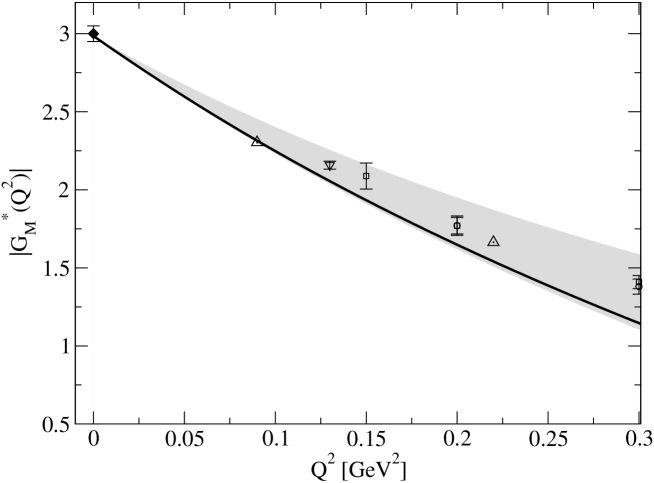
Figure 2: The momentum transfer dependence of the magnetic dipole form factor $\mathcal{G}_{M}^{*}(Q^{2})$: The solid line represents the $\mathcal{O}(\epsilon^{3})$ SSE result [1] as discussed in the text, the gray shaded band indicates the uncertainty of this result when neglecting higher order effects. Data points are taken from [15] (diamond), [16] (triangle up), [17] (triangle down), [18] (square) and [19] (circle).

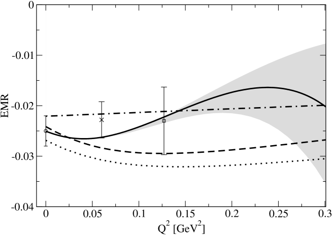
Figure 3: Momentum transfer dependence of the ratio of the electric quadrupole to the magnetic dipole form factor EMR$(Q^{2})$: The solid line represents the $\mathcal{O}(\epsilon^{3})$ SSE result [1] as discussed in the text, the gray shaded band indicates the uncertainty of this result when neglecting higher order effects. The dashed-dotted (MAID [14]), dashed (DMT [14]) and dotted (Sato-Lee [13]) curves are model predictions. Experimental date are from MAMI (real photon point [15] and $Q^{2}=0.06$GeV² [20]) and OOPS [4] ($Q^{2}=0.127$GeV²).

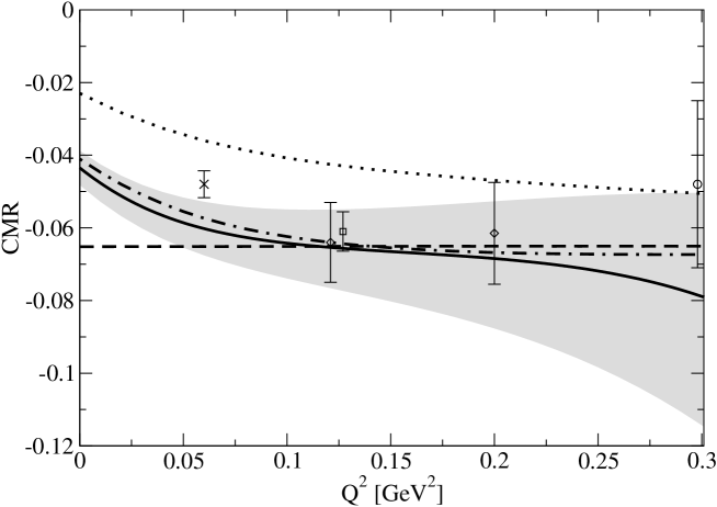
Figure 4: Momentum transfer dependence of the ratio of the Coulomb quadrupole to the magnetic dipole form factor CMR$(Q^{2})$: The solid line represents the $\mathcal{O}(\epsilon^{3})$ SSE result [1] as discussed in the text, the gray shaded band indicates the uncertainty of this result when neglecting higher order effects. The dashed-dotted (MAID [14]), dashed (DMT [14]) and dotted (Sato-Lee [13]) curves are model predictions. The data-points shown are from refs.[20] (cross), [21] (diamonds), [22] (circles) and [4] (square).

4 Acknowledgements

We thank Aron M. Bernstein ans Costas N. Papanicolas, the organizers of this workshop, for giving us the opportunity to present our results. This research is part of the EU Integrated Infrastructure Initiative Hadron Physics under contract number RII3-CT-2004-506078.

References

- [1] T.A. Gail and T.R. Hemmert, Eur. Phys. J. A28:91-105 (2006).
- [2] G.C. Gellas, T.R. Hemmert, C.N. Ktorides and G.I. Poulis, Phys. Rev. D60:054022 (1999).
- [3] H.F. Jones and M.D. Scadron, Annals Phys.81:1-14 (1973).
- [4] N.F. Sparveris et al. (OOPS Collaboration), Phys. Rev. Lett. 94:022003 (2005).
- [5] S. Eidelman et al. (Particle Data Group), Phys. Lett. B592:1 (2004).
- [6] V. Bernard, N. Kaiser, J. Kambor, U.-G. Meißner, Nucl. Phys. B388:315-345 (1992).
- [7] T.R. Hemmert, B.R. Holstein and J. Kambor,. J. Phys. G24:1831-1859 (1998).
- [8] V. Pascalutsa and M. Vanderhaeghen, Phys. Rev. D73:034003 (2006).
- [9] V. Pascalutsa and D.R. Phillips, Phys. Rev. C67:055202 (2003).
- [10] V. Bernard, H.W. Fearing, T.R. Hemmert and U.-G. Meißner, Nucl. Phys. A635:121-145 (1998), Erratum-ibid. A642:563-563 (1998) and T.R. Hemmert and W. Weise, Eur. Phys. J. A15:487-504 (2002).
- [11] J. Gasser, M.E. Sainio, A. Svarc, Nucl. Phys. B307:779 (1988) and B. Kubis and U.-G. Meißner, Nucl. Phys. A679:698-734 (2001).
- [12] C. Alexandrou, et al., Phys. Rev. Lett. 94:021601 (2005).
- [13] T. Sato and T.S.H. Lee, Phys. Rev. C63:055201 (2001) and T. Sato and T.S.H. Lee, Phys. Rev. C54:2660-2684 (1996).
-
[14]
S.S. Kamalov, et al., Phys. Rev. Lett. 83:4494 (1999) and Phys. Rev. C 64:032201 (2001).
D. Drechsel, O. Hanstein, S.S. Kamalov and L. Tiator, Nucl. Phys. A645:145 (1999).
http://www.kph.uni-mainz.de/MAID - [15] R. Beck et al., Phys. Rev. C61:035204 (2000).
- [16] S. Stein et al., Phys. Rev. D12:1884 (1975).
- [17] L. Tiator, D. Drechsel, S.S. Kamalov and S.N. Yang, Eur. Phys. J. A17:357-363 (2003).
- [18] K. Bätzner et al., Phys. Lett. B39:575-578 (1972).
- [19] W. Bartel et al., Phys. Lett. B28:148-151 (1968).
- [20] S. Stave et al. [nucl-ex/0604013].
- [21] Th. Pospischil et al., Phys. Rev. Lett. 86:2959-2962 (2001) and D. Elsner et al, Eur. Phys. J. A27:91-97 (2006).
- [22] R. Siddle et al., Nucl. Phys. B35:93-119 (1971) and K. Baetzner et al., Nucl. Phys. B76:1-14 (1974).