Nuclear dynamics in time-dependent picture

Abstract

Using the time-dependent theory of quantum mechanics, we investigate nuclear electric dipole responses. The time evolution of a wave function is explicitly calculated in the coordinate-space representation. The particle continuum is treated with the absorbing boundary condition. Calculated time-dependent quantities are transformed into those of familiar energy representation. We apply the method to a three-body model for ¹¹Li and to the mean-field model for ²²O, then discuss properties of $E1$ response.

1 Time-dependent method for nuclear responses

Atomic nuclei exhibit a variety of responses to different experimental probes; Coulomb and nuclear excitations, spin- and isospin-dependent probes, high- and low-energy reactions. In order to investigate properties of these nuclear excitations, it is useful to study response function for a probe (external) operator of interest. Normally, these quantum many-body problems are theoretically studied using the energy representation, in which calculations are carried out by either diagonalizing the Hamiltonian matrices or solving differential equations with a fixed energy. These approaches are advantageous when we are interested in states within a limited energy range. However, when we calculate response functions in a wide energy range, the energy representation may not be the best choice. Occasionally, the time representation provides more efficient numerical approaches to quantum problems. In this paper, instead of taking the time-independent (energy-dependent) framework, we present time-dependent approaches to nuclear response functions, and show their advantages and usefulness.

1.1 Time-dependent equation with absorbing boundary

The quantum mechanical problems are often described by the eigenvalue equation,

$$\hat{H}|\Psi\rangle=E|\Psi\rangle.$$ (1)

Since this stationary Schrödinger equation is derived from the time-dependent equation

$$i\hbar\frac{\partial}{\partial t}|\Psi(t)\rangle=\hat{H}|\Psi(t)\rangle,$$ (2)

these two equations should provide the same information if we could solve Eq. (1) for all the energies $E$ and solve Eq. (2) for an infinitely long period of time. However, in practice, we need to truncate either the energy range or the period of time propagation. Therefore, these two approaches have advantages and disadvantages, complimentary to each other. The stationary equation, Eq. (1), is suitable for precise calculation of eigenstates in a small energy range. In contrast, the time-dependent one, Eq. (2), will be superior in practice, when we are interested in a bulk property of response function for an extended energy range. The energy resolution obtained in the calculation is, roughly speaking, inversely proportional to the period of time propagation; $\Delta E\approx\hbar/T$. In general, longer the time propagation is, more precise energy the calculation can predict. However, for resonance states with positive energies, the time period $T$ can be safely truncated without much loss of the accuracy, because the states possess a finite width.

For the positive-energy states, we must deal with a problem of the boundary condition. For the time-dependent framework, since the asymptotic form of the wave function becomes a superposition of a variety of momentum eigenstates, solving the time-dependent Schrödinger equation (2) with a proper continuum boundary condition seems to be a very difficult task. However, the use of the absorbing complex potential provides a practical approach to the problem Kosloff and Kosloff (1986); Neuhasuer and Baer (1989); Seideman and Miller (1992); Muga et al. (2004). We use the complex potential to impose an approximate outgoing boundary condition on calculated time-dependent wave functions. This is simply done by replace Eq. (2) by

$$i\hbar\frac{\partial}{\partial t}|\Psi(t)\rangle=\left(\hat{H}-iW(\vec{r})\right)|\Psi(t)\rangle,$$ (3)

where $-iW(\vec{r})$ is a coordinate-dependent imaginary potential. Suppose we calculate the wave function $|\Psi(t)\rangle$ as a function of time $t$ with an initial state $|\Psi_{\text{in}}\rangle$ that is localized in space. $W(\vec{r})$ must be zero in the region of $\Psi_{\text{in}}(\vec{r})\neq 0$. while it is either zero or positive outside of this region. In addition, $\nabla W(\vec{r})$ should be small to prevent the reflection, but simultaneously $W(\vec{r})$ should be large enough to absorb all the outgoing waves. As long as these conditions are satisfied, in the region of $\Psi_{\text{in}}(\vec{r})\neq 0$, the wave function, $\Psi(\vec{r},t)$, obtained by solving Eq. (3) is identical to the solution of Eq. (2) with the outgoing boundary condition. Since small reflection of the waves by the potential $-iW$ is inevitable, this boundary condition is approximate, however, we have confirmed that the approximation is good enough to produce results indistinguishable from those of the exact boundary condition Nakatsukasa and Yabana (2001); Ueda et al. (2002); Nakatsukasa and Yabana (2005).

2 Applications

2.1 Three-body model: Coulomb breakup of ¹¹Li

In this section, we apply the time-dependent method to Coulomb breakup reaction of the two-neutron-halo nucleus, ¹¹Li. In the perturbative regime, properties of the Coulomb excitation are primarily determined by $dB(E1)/dE$ values. Strong soft $E1$ excitation in ¹¹Li were previously reported at MSU Ieki et al. (1993), at RIKEN Shimoura et al. (1995), and at GSI Zinser et al. (1997). However, these data seem to be inconsistent with each other. Recently, the experiment has been performed at RIKEN with much higher statistics Nakamura et al. (2006). The new data indicate a strong $E1$ peak around $E_{\text{x}}=0.6$ MeV.

The $B(E1)$ strength distribution is defined by

$$\frac{dB(E1)}{dE}=\sum_{\mu}\sum_{E^{\prime}}\delta(E-E^{\prime})\left|\langle\Psi_{E^{\prime}}|M_{1\mu}|\Psi_{0}\rangle\right|^{2},$$ (4)

where $|\Psi_{0}\rangle$ and $|\Psi_{E}\rangle$ are the ground and excited states of energy $E$, respectively. $M_{1\mu}$ is the $E1$ operator with a recoil charge. This quantity is rewritten in the following way:

$$\frac{dB(E1)}{dE} = \frac{1}{\pi\hbar}\text{Re}\sum_{\mu}\int_{0}^{\infty}dte^{iEt/\hbar}\langle\Psi_{0}|M^{\dagger}_{1\mu}e^{-iHt/\hbar}M_{1\mu}|\Psi_{0}\rangle$$ (5)

$$= \frac{1}{\pi\hbar}\text{Re}\sum_{\mu}\int_{0}^{\infty}dte^{iEt/\hbar}\langle\tilde{\Psi}^{\mu}(0)|\tilde{\Psi}^{\mu}(t)\rangle.$$ (6)

Thus, $B(E1)$ strength distribution can be calculated using the time propagation of the state $|\tilde{\Psi}^{\mu}(t)\rangle$. The initial state is given by $|\tilde{\Psi}^{\mu}(0)\rangle=M_{1\mu}|\Psi_{0}\rangle$ in Eq. (6). It should be noted that, in the time-dependent method, we do not need to construct the energy eigenstates, $|\Psi_{E}\rangle$.

We adopt the following Hamiltonian for ¹¹Li, neglecting the recoil of the ⁹Li core.

$$H=-\frac{\hbar^{2}}{2m}\nabla_{1}^{2}-\frac{\hbar^{2}}{2m}\nabla_{2}^{2}+V_{nC}(r_{1})+V_{nC}(r_{2})+V_{nn}(|\mathbf{r}_{1}-\mathbf{r}_{2}|),$$ (7)

where $m$ indicates the neutron mass. The interaction potential between neutron-⁹Li ($V_{nC}$) and that of neutron-neutron ($V_{nn}$) are both in the Woods-Saxon form with radius of 2.3 fm and the diffuseness of 0.6 fm. Occupied orbitals, $\phi_{s}(r_{1})$ and $\phi_{s}(r_{2})$, are excluded from the model space ($H\rightarrow PHP$), using a projection operator,

$$P\equiv\left\{1-|\phi_{s}(1)\rangle\langle\phi_{s}(1)|\right\}\left\{1-|\phi_{s}(2)\rangle\langle\phi_{s}(2)|\right\}.$$ (8)

The ground state is assumed to be a spin-singlet state, thus must be symmetric in the coordinate space, $\Psi_{0}(\vec{r}_{1},\vec{r}_{2})=\Psi_{0}(\vec{r}_{2},\vec{r}_{1})$. The depth of $V_{nC}$ potentials are adjusted so as to reproduce the two-neutron separation energy of 0.3 MeV. Numerical calculations are performed using the partial-wave expansion with respect to the $n$-$C$ coordinates, $\vec{r}_{1}$ and $\vec{r}_{2}$. The Lagrange-mesh method is used for the radial coordinate Baye and Heenen (1986). Since the initial state $\tilde{\Psi}^{\mu}(0)$, which decays in time, is excited in the continuum, we add the absorbing potentials, $-iW(r_{1})$ and $-iW(r_{2})$, to the Hamiltonian of Eq. (7). These imaginary potentials should be non-zero only where the initial wave function vanishes ($r_{1},r_{2}>R$). As the time passes, the two neutrons slowly go away to the infinity ($r_{1},r_{2}\rightarrow\infty$), and are absorbed by these potentials.

Figure 1: Calculated $B(E1)$ distribution for ¹¹Li.

Calculated $E1$ strength distribution, $dB(E1)/dE$, is shown in Fig. 1. The attractive neutron-neutron interaction, $V_{nn}$, is chosen to be weaker than the one to reproduce the $n$-$n$ scattering length in free space Esbensen et al. (1997). The peak position is around $E_{\text{x}}=0.8$ MeV. This should be compared to the recent measurement, $E_{\text{x}}=0.6$ MeV Nakamura et al. (2006). In order to reproduce the observed peak position more precisely, we may need to improve the Hamiltonian and the ground state of ¹¹Li.

2.2 TDHF: Giant dipole resonances in ²²O

Calculations based on the time-dependent Schrödinger equation of Eq. (3) becomes increasingly difficult as the particle number increases. A possible way to avoid this difficulty is to resort to the density functional (mean-field) theory. In this section, we use the time-dependent Hartree-Fock (TDHF) method with the Skyrme interaction to study the dipole response in neutron-rich Oxygen isotope, ²²O.

Although the TDHF wave packet is capable of describing nuclear dynamics of the large-amplitude nature, it is not an easy task to requantize the TDHF trajectories. Thus, we focus our discussion on its small-amplitude (perturbative) limit. This is nothing but the well-known random-phase approximation (RPA) which has been extensively utilized for studies of both high-energy giant resonances and low-energy collective excitations Ring and Schuck (1980). Here, we calculate it in the time-dependent manner.

The RPA equation for the linear response with the density-dependent interaction is usually derived from the small-amplitude approximation of the time-dependent Hartree-Fock (TDHF) theory. Thus, we should be able to obtain the same information from the time propagation of a Slater determinant. Let us assume that the state is initially the ground (HF) state, then a perturbative external field, $V_{\text{ext}}(t)$, is switched on. Each single-particle orbital follows the TDHF equation

$$i\hbar\frac{\partial}{\partial t}|\psi_{i}(t)\rangle=\left(\hat{h}[\rho]+V_{\text{ext}}(t)\right)|\psi_{i}(t)\rangle,\quad i=1,\cdots,A,$$ (9)

where $\hat{h}[\rho]$ is the single-particle Hamiltonian. The single-particle states are now slightly deviated from its initial states, $|\phi_{i}\rangle$:

$$|\psi_{i}(t)\rangle=\left(|\phi_{i}\rangle+|\delta\psi_{i}(t)\rangle\right)e^{-i\epsilon_{i}t/\hbar},$$ (10)

where $\epsilon_{i}$ are the HF single-particle energies at the ground state. Decomposition of $|\delta\psi_{i}(t)\rangle$ into normal modes leads to the RPA eigenvalue equations. Instead of doing this, we may simply calculate the time-dependent $E1$ dipole moment,

$$D_{1\mu}(t)=\sum_{i=1}^{A}\langle\psi_{i}(t)|M_{1\mu}|\psi_{i}(t)\rangle\approx\text{Re}\sum_{i=1}^{A}\langle\phi_{i}|M_{1\mu}|\delta\psi_{i}(t)\rangle.$$ (11)

Then, the Fourier transform of Eq. (11) provides information of eigenenergies and transition strength of the RPA normal modes.

We perform the TDHF calculations using the three-dimensional (3D) Cartesian mesh representation. The full Skyrme functional with the SGII parameter set is adopted, which preserves the Galilean invariance. The time-dependent method provides an efficient tool to calculate the $E1$ strength function for a wide range of energy. In fact, to diagonalize the RPA matrix in the 3D coordinate space is a time-consuming procedure Muta et al. (2002); Imagawa and Hashimoto (2003); Inakura et al. (2004). The small-amplitude TDHF gives a feasible alternative.

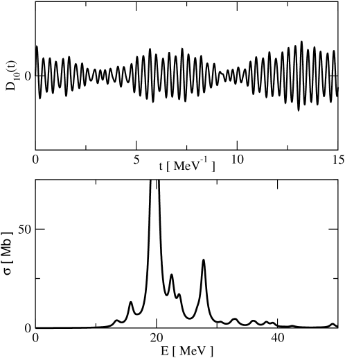
Figure 2: (Top) Calculated time-dependent $E1$ moment for ²²O. (Bottom) Calculated photoabsorption cross section for ²²O.

In the top panel of Fig. 2, we show the time evolution of $D_{10}(t)$ for ²²O, Eq. (11), with an instantaneous $E1$ external field, $V_{\text{ext}}(t)=\eta M_{10}\delta(t)$, where $\eta$ is an arbitrary parameter. The time evolution is calculated up to $t=20\ \hbar/$MeV. Here, we do not use the absorbing potential. Therefore, the particle continuum is discretized, leading to discrete peaks in the strength function. Then, we calculate the Fourier transform of $D_{10}(t)$ with complex energy, $E+i\Gamma$ with $\Gamma=1$ MeV. The imaginary part of the energy gives a smoothing width to every peak. In the bottom panel of Fig. 2, photoabsorption cross section, calculated in this way, is presented. The main peak position is almost the same as that of ¹⁶O Nakatsukasa and Yabana (2005). Experimental data obtained at GSI suggest a low-energy peak around $E_{\text{x}}=9$ MeV Leistenschneider et al. (2001). The present calculation produces the lowest peak at 13 MeV. This discrepancy may be due to the fact that the neutron separation energy is too large in the calculation with the SGII parameter set. The main peak position around $E_{\text{x}}=20$ MeV has not been confirmed experimentally, however, the result is similar to that of the relativistic RPA calculation Vretenar et al. (2001).

3 Summary

We present the time-dependent method to study nuclear response functions. The continuum can be properly treated with the absorbing boundary condition. The method is first applied to a three-body model to investigate $B(E1)$ distribution in ¹¹Li. The calculation produces a strong $E1$ strength at low energy, however the peak position is slightly too high compared to the experiment. It seems to be necessary to improve the model Hamiltonian in order to reproduce the peak position quantitatively. We next apply the time-dependent Hartree-Fock analysis to giant resonances. We show $E1$ resonances in ²²O, using the SGII Skyrme functional. The main peak is consistent with the relativistic RPA calculation. The position of the low-energy peak is calculated to be higher than the experiment by about 4 MeV. The time-dependent method is an efficient tool to investigate nuclear response function, especially for its bulk structure in a wide range of energy.

References

- Kosloff and Kosloff (1986) R. Kosloff, and D. Kosloff, J. Comp. Phys. 63, 363 (1986).
- Neuhasuer and Baer (1989) D. Neuhasuer, and M. Baer, J. Chem. Phys. 90, 4351 (1989).
- Seideman and Miller (1992) T. Seideman, and W. Miller, J. Chem. Phys. 97, 2499 (1992).
- Muga et al. (2004) J. G. Muga, J. P. Palao, B. Navarro, and I. L. Egusquiza, Phys. Rep. 395, 357 (2004).
- Nakatsukasa and Yabana (2001) T. Nakatsukasa, and K. Yabana, J. Chem. Phys. 114, 2550 (2001).
- Ueda et al. (2002) M. Ueda, K. Yabana, and T. Nakatsukasa, Phys. Rev. C 67, 014606 (2002).
- Nakatsukasa and Yabana (2005) T. Nakatsukasa, and K. Yabana, Phys. Rev. C 71, 024301 (2005).
- Ieki et al. (1993) K. Ieki, et al., Phys. Rev. Lett. 70, 730 (1993).
- Shimoura et al. (1995) S. Shimoura, et al., Phys. Lett. B 348, 29 (1995).
- Zinser et al. (1997) M. Zinser, et al., Nucl. Phys. A 619, 151 (1997).
- Nakamura et al. (2006) T. Nakamura, et al., Phys. Rev. Lett. 96, 252502 (2006).
- Baye and Heenen (1986) D. Baye, and P.-H. Heenen, J. Phys. A 19, 2041 (1986).
- Esbensen et al. (1997) H. Esbensen, G. F. Bertsch, and K. Hencken, Phys. Rev. C 56, 3054 (1997).
- Ring and Schuck (1980) P. Ring, and P. Schuck, The nuclear many-body problems, Springer-Verlag, New York, 1980.
- Muta et al. (2002) A. Muta, J.-I. Iwata, Y. Hashimoto, and K. Yabana, Prog. Theor. Phys. 108, 1065 (2002).
- Imagawa and Hashimoto (2003) H. Imagawa, and Y. Hashimoto, Phys. Rev. C 67, 037302 (2003).
- Inakura et al. (2004) T. Inakura, et al., Int. J. Mod. Phys. E 13, 157 (2004).
- Leistenschneider et al. (2001) A. Leistenschneider, et al., Phys. Rev. Lett. 86, 5442 (2001).
- Vretenar et al. (2001) D. Vretenar, N. Paar, P. Ring, and G. A. Lalazissis, Nucl. Phys. A 692, 496 (2001).