Variation after Particle-Number Projection for the HFB Method with the Skyrme Energy Density Functional

Abstract

Variation after particle-number restoration is incorporated for the first time into the Hartree-Fock-Bogoliubov framework employing the Skyrme energy density functional with zero-range pairing. The resulting projected HFB equations can be expressed in terms of the local gauge-angle-dependent densities. Results of projected calculations are compared with those obtained within the Lipkin-Nogami method in the standard version and with the Lipkin-Nogami method followed by exact particle-number projection.

I Introduction

Pairing correlations affect properties of atomic nuclei in a profound way [Boh75] ; [RS80] ; [Bri05] ; [Dea03] . They impact nuclear binding, properties of nuclear excitations and decays, and dramatically influence the nuclear collective motion. In particular, pairing plays a crucial role in exotic, weakly bound nuclei in which the magnitude of the chemical potential is close to that of the pairing gap. In such systems, a naive independent single-particle picture breaks down and the pair scattering, also involving the continuum part of the phase space, can determine the very nuclear existence [Dob98c] .

Many aspects of nuclear superfluidity can be successfully treated within the independent quasiparticle framework by applying the Bardeen-Cooper-Schrieffer (BCS) [Bar57] or Hartree-Fock-Bogoliubov (HFB) approximations [RS80] . The advantage of the mean-field approach to the pairing problem lies in its simplicity that allows for a straightforward interpretation in terms of pairing fields and deformations (pairing gaps) associated with the spontaneous breaking of the gauge symmetry. However, this simplicity comes at a cost. In the intrinsic-system description, the gauge angle associated with the particle-number operator is fixed; hence, the particle-number invariance is internally broken [Boh75] ; [RS80] ; [Bri05] . Therefore, to relate to experiment, the particle-number symmetry needs to be, in principle, restored.

Some observables, like masses, radii, or deformations are not very strongly affected by the particle-number-symmetry restoration, while some other ones, like even-odd mass staggering or pair-transfer amplitudes are influenced significantly. Moreover, quantitative impact of the particle-number projection (PNP) depends on whether the pairing correlations are strong (open-shell systems) or weak (near closed shells). Therefore, methods of restoring the particle-number symmetry must be implemented in studies of pairing correlations. This can be done on various levels [RS80] ; [Flo97] , including the quasiparticle random phase approximation, Kamlah expansion [Kam68] ; [Zhe92] , Lipkin-Nogami (LN) method [Lip60] ; [Nog64] ; [Gal94] ; [Rei96] ; [Cwi96] ; [Val97] ; [Val00a] ; [Ben00e] ; [Sto03] , the particle-number projection after variation (PNPAV) [RS80] ; [Ang02] , the projected LN method (PLN) [Dob93] ; [Mag93] ; [Ang02] ; [Sto03] ; [Sam04] , and the variation after particle-number projection (VAPNP) [Die64] ; [Sch87] ; [She00a] ; [Ang01a] ; [Ang02] .

In this work, we concentrate on the VAPNP method. Recently, it has been shown [She00a] that the total energy in the HFB+VAPNP approach can be expressed as a functional of the unprojected HFB density matrix and pairing tensor. Its variation leads to a set of HFB-like equations with modified self-consistent fields. The method has been illustrated within schematic models [She02] , and also implemented in the HFB calculations with the finite-range Gogny force [Ang01a] ; [Ang02] . Here, we adopt it for the Skyrme energy-density functionals and zero-range pairing forces; in this case the building blocks of the method are the local particle-hole and particle-particle densities and mean fields. In the present study, the HFB equations are solved by using the Harmonic Oscillator (HO) basis, but the formalism can be straightforwardly applied with the Transformed Harmonic Oscillator (THO) basis [Sto03] ; [Sto05] , which helps maintain the correct asymptotic behavior of the single-quasiparticle wave functions.

The paper is organized as follows. Section II gives a brief overview of the HFB theory and defines the densities and fields entering the formalism. Section III extends the VAPNP method of Ref. [She02] to the case of the HFB theory with Skyrme interaction. The technical details pertaining to the Skyrme HFB+VAPNP method are given in Sec. IV, while Sec. V contains an illustrative example of calculations for the Ca and Sn isotopes. In particular, the LN and PLN approximations are compared to the VAPNP results. Summary and discussion are given in Section VI. Preliminary results of our VAPNP calculations were presented in Ref. [Sto05b] .

II The HFB method

The many-body Hamiltonian of a system of fermions is usually expressed in terms of a set of annihilation and creation operators $(c,c^{\dagger})$:

$$H = \sum_{nn^{\prime}}e_{nn^{\prime}}~{}c_{n}^{\dagger}c_{n^{\prime}}$$ (1)

$$+ \tfrac{1}{4}\sum_{nn^{\prime}mm^{\prime}}V_{nn^{\prime}mm^{\prime}}~{}c_{n}^{\dagger}c_{n^{\prime}}^{\dagger}c_{m^{\prime}}c_{m},$$

where

$$V_{nn^{\prime}mm^{\prime}}=\langle nn^{\prime}|V|mm^{\prime}-m^{\prime}m\rangle$$ (2)

are the anti-symmetrized two-body interaction matrix-elements.

In the HFB method, the ground-state wave function is the quasiparticle vacuum $|\Phi\rangle,$ defined as $\alpha_{k}|\Phi\rangle=0$, where the quasiparticle operators $(\alpha,\alpha^{\dagger})$ are connected to the original particle operators via the Bogoliubov transformation

$$\quad\quad\alpha_{k} = \sum_{n}\left(U_{nk}^{\ast}c_{n}+V_{nk}^{\ast}c_{n}^{\dagger}\right),$$ (3)

$$\quad\quad\alpha_{k}^{\dagger} = \sum_{n}\left(V_{nk}c_{n}+U_{nk}c_{n}^{\dagger}\right),$$ (4)

where the matrices $U$ and $V$ satisfy the unitarity and completeness relations:

$$U^{\dagger}U+V^{\dagger}V=I, UU^{\dagger}+V^{\ast}V^{T}=I,$$ (5)

$$U^{T}V+V^{T}U=0, UV^{\dagger}+V^{\ast}U^{T}=0.$$ (6)

II.1 The HFB equations

In terms of the density matrix $\rho$ and pairing tensor $\kappa$, defined as

$$\rho=V^{\ast}V^{T},\quad\kappa=V^{\ast}U^{T}=-UV^{\dagger},$$ (7)

the HFB energy is expressed as an energy functional:

$$E[\rho,\kappa] = \frac{\langle\Phi|H|\Phi\rangle}{\langle\Phi|\Phi\rangle}$$ (8)

$$= {\rm Tr}\left[\left(e+\tfrac{1}{2}\Gamma\right)\rho\right]-\tfrac{1}{2}{\rm Tr}\left[\Delta\kappa^{\ast}\right],$$

where

$$\Gamma_{nm} = \sum_{n^{\prime}m^{\prime}}V_{nn^{\prime}mm^{\prime}}\rho_{m^{\prime}n^{\prime}},$$ (9)

$$\Delta_{nn^{\prime}} = \tfrac{1}{2}\sum_{mm^{\prime}}V_{nn^{\prime}mm^{\prime}}\kappa_{mm^{\prime}}.$$ (10)

The variation of the HFB energy (8) with respect to $\rho$ and $\kappa$ yields the HFB equations:

$${\cal H}\left(\begin{array}[]{c}U_{k}\\ V_{k}\end{array}\right)=E_{k}\left(\begin{array}[]{c}U_{k}\\ V_{k}\end{array}\right),$$ (11)

where

$${\cal H}=\left(\begin{array}[]{cc}e+\Gamma-\lambda&\Delta\\ -\Delta^{\ast}&-(e+\Gamma)^{\ast}+\lambda\end{array}\right),$$ (12)

$U_{k}$ and $V_{k}$ are the $k$th columns of matrices $U$ and $V$, respectively, and $E_{k}$ is a positive quasiparticle energy eigenvalue. Since the HFB state $|\Phi\rangle$ violates the particle-number symmetry, the Fermi energy $\lambda$ is introduced to fix the average particle number.

II.2 The Skyrme HFB method

For the zero-range Skyrme forces, the HFB formalism can be written directly in the coordinate representation [Bul80] ; [Dob84] ; [Per04] by introducing particle and pairing densities

$$\rho({\bm{r}}\sigma,{\bm{r}^{\prime}}\sigma^{\prime}) = \tfrac{1}{2}\rho({\bm{r}},{\bm{r}}^{\prime})\delta_{\sigma\sigma^{\prime}}$$ (13)

$$+ \tfrac{1}{2}\sum_{i}(\sigma|\sigma_{i}|\sigma^{\prime})\rho_{i}({\bm{r}},{\bm{r}}^{\prime}),$$

$$\tilde{\rho}({\bm{r}}\sigma,{\bm{r}^{\prime}}\sigma^{\prime}) = \tfrac{1}{2}\tilde{\rho}({\bm{r}},{\bm{r}}^{\prime})\delta_{\sigma\sigma^{\prime}}$$ (14)

$$+ \tfrac{1}{2}\sum_{i}(\sigma|\sigma_{i}|\sigma^{\prime})\tilde{\rho}_{i}({\bm{r}},{\bm{r}}^{\prime}),$$

which explicitly depend on spin. The use of the pairing density $\tilde{\rho}$,

$$\tilde{\rho}({\bm{r}}\sigma,{\bm{r}^{\prime}}\sigma^{\prime})=-2\sigma^{\prime}\kappa({\bm{r},}\sigma,{\bm{r}^{\prime},}-\sigma^{\prime}),$$ (15)

instead of the pairing tensor $\kappa$ is convenient when restricting to time-even quasiparticle states where both $\rho$ and $\tilde{\rho}$ are hermitian and time-even [Dob84] .

The densities $\rho$ and $\tilde{\rho}$ can be expressed in the single-particle basis:

$$\rho({\bm{r}}\sigma,{\bm{r}^{\prime}}\sigma^{\prime}) = \sum_{nn^{\prime}}\rho_{nn^{\prime}}~{}\psi_{n^{\prime}}^{\ast}({\bm{r}^{\prime}},\sigma^{\prime})\psi_{n}({\bm{r}},\sigma),$$ (16)

$$\tilde{\rho}({\bm{r}}\sigma,{\bm{r}^{\prime}}\sigma^{\prime}) = \sum_{nn^{\prime}}\tilde{\rho}_{nn^{\prime}}~{}\psi_{n^{\prime}}^{\ast}({\bm{r}^{\prime}},\sigma^{\prime})\psi_{n}({\bm{r}},\sigma),$$ (17)

where $\rho_{n^{\prime}n}$ and $\tilde{\rho}_{n^{\prime}n}$ are the corresponding density matrices. In this study, we take ${\psi_{n}({\bm{r}},\sigma)}$ as a set of the HO wave functions.

The building blocks of the Skyrme HFB method are the local densities, namely the particle density $\rho({\bm{r}})$, kinetic energy density $\tau({\bm{r}})$, and spin-current density ${\mathsf{J}}_{ij}({\bm{r}})$:

$$\begin{array}[]{ccl}\rho({\bm{r}})&=&\rho({\bm{r}},{\bm{r}}),\\ {}\hfil&&\\ \tau({\bm{r}})&=&\left.\nabla_{{\bm{r}}}\nabla_{{\bm{r}}^{\prime}}\rho({\bm{r}},{\bm{r}}^{\prime})\right|_{{\bm{r}}^{\prime}={\bm{r}}}\;,\\ {}\hfil&&\\ {\mathsf{J}}_{ij}({\bm{r}})&=&\tfrac{1}{2i}\left.\left(\nabla_{i}-\nabla_{i}^{\prime}\right)\rho_{j}({\bm{r}},{\bm{r}}^{\prime})\right|_{{\bm{r}}^{\prime}={\bm{r}}}\;,\end{array}$$ (18)

as well as the corresponding pairing densities $\tilde{\rho}({\bm{r}})$, $\tilde{\tau}({\bm{r}})$ and $\tilde{\mathsf{J}}_{ij}({\bm{r}})$.

In the coordinate representation, the Skyrme HFB energy (8) can be written as a functional of the local particle and pairing densities:

$$E[\rho,\tilde{\rho}]=\frac{\langle\Phi|H|\Phi\rangle}{\langle\Phi|\Phi\rangle}=\int d{\bm{r}}~{}{\cal H}({\bm{r}}).$$ (19)

The energy density ${\cal H}({\bm{r}})$ is a sum of the particle $H({\bm{r}})$ and pairing energy density $\tilde{H}({\bm{r}})$:

$${\cal H}({\bm{r}})=H({\bm{r}})+\tilde{H}({\bm{r}}).$$ (20)

The derivatives of $E[\rho,\tilde{\rho}]$ with respect to density matrices $\rho$ and $\tilde{\rho}$ define the self-consistent particle ($h$) and pairing ($\tilde{h}$) fields, respectively. The explicit expressions for $H({\bm{r}})$, $\tilde{H}({\bm{r}})$, $h({\bm{r}},\sigma,\sigma^{\prime})$, and $\tilde{h}({\bm{r}},\sigma,\sigma^{\prime})$ have been given in Ref. [Dob84] and will not be repeated here.

The Skyrme HFB equations can be written in the matrix form as:

$$\left(\begin{array}[]{cc}h-\lambda&\tilde{h}\\ \tilde{h}&-h+\lambda\end{array}\right)\left(\begin{array}[]{c}\varphi_{1,k}\\ \varphi_{2,k}\end{array}\right)=E_{k}\left(\begin{array}[]{c}\varphi_{1,k}\\ \varphi_{2,k}\end{array}\right),$$ (21)

where

$$h_{nn^{\prime}} = \frac{\partial E[\rho,\tilde{\rho}]}{\partial\rho_{n^{\prime}n}}$$ (22)

$$= \sum_{\sigma\sigma^{\prime}}\int d{\bm{r}}~{}\psi_{n}^{\ast}({\bm{r}},\sigma)h({\bm{r}},\sigma,\sigma^{\prime})\psi_{n^{\prime}}({\bm{r}},\sigma^{\prime}),$$

and

$$\tilde{h}_{nn^{\prime}} = \frac{\partial E[\rho,\tilde{\rho}]}{\partial\tilde{\rho}_{n^{\prime}n}}$$ (23)

$$= \sum_{\sigma\sigma^{\prime}}\int d{\bm{r}}~{}\psi_{n}^{\ast}({\bm{r}},\sigma)\tilde{h}({\bm{r}},\sigma,\sigma^{\prime})\psi_{n^{\prime}}({\bm{r}},\sigma^{\prime}),$$

and $\varphi_{1,k}$ and $\varphi_{2,k}$ are the upper and lower components, respectively, of the quasiparticle wave function corresponding to the positive quasiparticle energy $E_{k}$. After solving the HFB equations (21), one obtains the density matrices,

$$\rho_{nn^{\prime}}=\sum_{E_{k}>0}\varphi_{2,nk}\varphi^{*}_{2,n^{\prime}k},$$ (24)

$$\tilde{\rho}_{nn^{\prime}}=-\sum_{E_{k}>0}\varphi_{2,nk}\varphi^{*}_{1,n^{\prime}k},$$ (25)

which define the spatial densities (16) and (17) .

We note in passing that the derivation of the coordinate-space HFB equations [Dob84] is strictly valid only when the time-reversal symmetry is assumed. When the time-reversal symmetry is broken, one has to introduce additional real vector particle densities ${\bm{s}}$, ${\bm{j}}$, ${\bm{T}}$ [Eng75] , while the pairing densities acquire imaginary parts; see Ref. [Per04] for complete derivations.

III Variation after particle-number projection

III.1 The HFB+VAPNP method

It has been demonstrated [She00a] that the HFB+VAPNP energy,

$$E^{N}[\rho,\kappa] = \frac{\left\langle\Phi|HP^{N}|\Phi\right\rangle}{\left\langle\Phi|P^{N}|\Phi\right\rangle}$$ (26)

$$= \frac{\int d\phi\langle\Phi|{H}e^{i\phi({\hat{N}}-N)}|\Phi\rangle}{\int d\phi\langle\Phi|e^{i\phi({\hat{N}}-N)}|\Phi\rangle},$$

where $P^{N}$ is the particle-number projection operator,

$$P^{N}=\frac{1}{2\pi}\int d\phi\ e^{i\phi(\hat{N}-N)},$$ (27)

can be written as an energy functional of the unprojected densities (7).

The variation of Eq. (26) results in the HFB+VAPNP equations:

$${\cal H}^{N}\left(\begin{array}[]{c}U_{k}^{N}\\ V_{k}^{N}\end{array}\right)={\cal E}_{k}\left(\begin{array}[]{c}U_{k}^{N}\\ V_{k}^{N}\end{array}\right),$$ (28)

where

$${\cal H}^{N}=\left(\begin{array}[]{cc}\varepsilon^{N}+\Gamma^{N}+\Lambda^{N}&\Delta^{N}\\ -{(\Delta^{N})}^{\ast}&-(\varepsilon^{N}+\Gamma^{N}+\Lambda^{N})^{\ast}\end{array}\right).$$ (29)

Equations (28) and (29) have the same structure as Eqs. (11) and (12), except that the expressions for the VAPNP fields are now different [She00a] ; [She02] , i.e.,

$$\varepsilon^{N} = \tfrac{1}{2}\int d\phi\,\,y(\phi)\left\{Y(\phi){\rm Tr}[e\rho(\phi)]\right.$$ (30)

$$+ \left.[1-2ie^{-i\phi}\sin\phi\rho(\phi)]eC(\phi)\right\}+{\rm h.c.},$$

$$\Gamma^{N} = \tfrac{1}{4}\int d\phi\,\,y(\phi)\left\{Y(\phi){\rm Tr}[\Gamma(\phi)\rho(\phi)]\right.$$ (31)

$$+ \left.2[1-2ie^{-i\phi}\sin\phi\rho(\phi)]\Gamma(\phi)C(\phi)\right\}+{\rm h.c.},$$

$$\Delta^{N} = \tfrac{1}{2}\int d\phi\;y(\phi)e^{-2i\phi}C\left(\phi\right)\Delta(\phi)-(...)^{T},$$ (32)

$$\Lambda^{N} = -\tfrac{1}{4}\int d\phi\,\,y(\phi)\left\{Y(\phi){\rm Tr}[\Delta(\phi)\overline{\kappa}^{\ast}(\phi)]\right.$$ (33)

$$- \left.4ie^{-i\phi}\sin\phi\;C(\phi)\Delta(\phi)\overline{\kappa}^{\ast}(\phi)\right\}+{\rm h.c.},$$

with

$$\Gamma_{nm}(\phi) = \sum_{n^{\prime}m^{\prime}}V_{nn^{\prime}mm^{\prime}}\rho_{m^{\prime}n^{\prime}}(\phi),$$ (34)

$$\Delta_{nn^{\prime}}(\phi) = \tfrac{1}{2}\sum_{mm^{\prime}}V_{nn^{\prime}mm^{\prime}}\kappa_{mm^{\prime}}(\phi),$$ (35)

where, using the unit matrix $\hat{I}$,

$$\rho(\phi) = C(\phi)\rho,$$ (36)

$$\kappa(\phi) = C(\phi)\kappa,$$ (37)

$$\overline{\kappa}(\phi) = e^{2i\phi}C^{\dagger}(\phi)\kappa,$$ (38)

$$C(\phi) = e^{2i\phi}\left[1+\rho(e^{2i\phi}-1)\right]^{-1},$$ (39)

$$x(\phi) = \frac{1}{2\pi}\frac{e^{-i\phi N}\det(e^{i\phi}I)}{\sqrt{\det C(\phi)}},$$ (40)

$$y(\phi) = \frac{x(\phi)}{\int d\phi^{\prime}\,x(\phi^{\prime})},$$ (41)

and

$$Y(\phi) = \,ie^{-i\phi}\sin\phi\;C(\phi)$$ (42)

$$- i\int d\phi^{\prime}y(\phi^{\prime})e^{-i\phi^{\prime}}\sin\phi^{\prime}\;C(\phi^{\prime}).$$

After solving the HFB+VAPNP equations (28), one obtains the intrinsic density matrix and pairing tensor:

$$\rho=(V^{N})^{\ast}(V^{N})^{T},\quad\kappa=(V^{N})^{\ast}(U^{N})^{T}.$$ (43)

Finally, the total HFB+VAPNP energy is given by

$$E^{N}[\rho,\kappa] = \int d\phi~{}y(\phi)~{}{\rm Tr}\left(e\rho(\phi)+\tfrac{1}{2}\Gamma(\phi)\rho(\phi)\right)$$ (44)

$$- \int d\phi~{}y(\phi)~{}\tfrac{1}{2}{\rm Tr}\left(\Delta(\phi)\overline{\kappa}^{\ast}(\phi)\right).$$

The quantity $y(\phi)$ plays a role of an $N$-dependent metric. The integrands in Eqs. (30)–(32) take the familiar HFB limit at $\phi$=0, while the integrand in (33) vanishes ($\Lambda^{N}$ does not appear in the standard HFB approach).

III.2 The Lipkin-Nogami method

The LN method [Lip60] ; [Nog64] constitutes an astute and efficient way of performing an approximate VAPNP calculation. It can be considered [Flo97] as a variant of the second-order Kamlah expansion [Kam68] ; [Zhe92] , in which the VAPNP energy (26) is approximated by a simple expression,

$$E_{\text{LN}}=E[\rho,\tilde{\rho}]-\lambda_{2}(\langle\hat{N}^{2}\rangle-N^{2}),$$ (45)

with $\lambda_{2}$ depending on the HFB state $|\Phi\rangle$ and representing the curvature of the VAPNP energy with respect to the particle number. The role of $\lambda_{2}$ in the Kamlah and LN methods differs. In the former, $\lambda_{2}$ is varied along with variations of the HFB state $|\Phi\rangle$, while in the latter, this variation is neglected. Had the second-order Kamlah expression (45) been exact, the variation of $\lambda_{2}$ would have been fully justified and the method would be giving the exact VAPNP energy. However, since the second-order expression is, in practical applications, never exact, it is usually more reasonable to adopt the LN philosophy, in which one rather strives to find the best estimate of the curvature $\lambda_{2}$ instead of finding it variationally in an approximate way.

When the HFB method is applied to a given Hamiltonian, values of $\lambda_{2}$ can be estimated by calculating new mean-field potentials, $\Gamma^{\prime}$ and $\Delta^{\prime}$, that are analogous to the standard mean fields of Eqs. (9) and (10); see, e.g., Refs. [Flo97] ; [Sto03] . However, apart from studies based on the Gogny Hamiltonian [Ang02] , such a formula was not used, because most often the self-consistent calculations are performed within the density functional approach or by using different interactions in the particle-hole and particle-particle channels. Moreover, in most studies, such as those of Ref. [Gal94] , the terms in $\lambda_{2}$ originating from the particle-hole channel are simply disregarded.

Similarly, as in our previous study [Sto03] , here we adopt an efficient phenomenological way of estimating the curvature $\lambda_{2}$ from the seniority-pairing expression,

$$\lambda_{2}=\frac{G_{\text{eff}}}{4}\frac{{\rm Tr^{\prime}}(1-\rho)\kappa~{}{\rm Tr^{\prime}}\rho\kappa-2~{}{\rm Tr}(1-\rho)^{2}\rho^{2}}{\left[{\rm Tr}\rho(1-\rho)\right]^{2}-2~{}{\rm Tr}\rho^{2}(1-\rho)^{2}},$$ (46)

where the effective pairing strength,

$$G_{\text{eff}}=-\frac{\bar{\Delta}^{2}}{E_{\text{pair}}},$$ (47)

is determined from the HFB pairing energy,

$$E_{\text{pair}}=-\frac{1}{2}{\rm Tr}\Delta\kappa^{*},$$ (48)

and the average pairing gap ,

$$\bar{\Delta}=\frac{{\rm Tr^{\prime}}\Delta\rho}{{\rm Tr}\rho}\,.$$ (49)

Expression (46) pertains to a system of particles occupying single-particle levels with fixed (non-self-consistent) energies and interacting with a seniority pairing interaction. In our method, this expression is used to probe the density of self-consistent energies that determine the curvature $\lambda_{2}$. All quantities defining $\lambda_{2}$ in Eq. (46) depend on the self-consistent solution and microscopic interaction, while the effective pairing strength $G_{\text{eff}}$ is only an auxiliary quantity. The quality of the prescription for calculating $\lambda_{2}$ can be tested against the exact VAPNP results (see Sec. V).

III.3 The Skyrme HFB+VAPNP method

Following the VAPNP procedure of Sec. III.1, one can develop the Skyrme HFB+VAPNP equations by introducing the gauge-angle-dependent transition density matrices:

$$\rho({\bm{r}}\sigma,{\bm{r}^{\prime}}\sigma^{\prime},\phi) = \sum_{nn^{\prime}}\rho_{nn^{\prime}}(\phi)~{}\psi_{n^{\prime}}^{\ast}({\bm{r}^{\prime}},\sigma^{\prime})\psi_{n}({\bm{r}},\sigma),$$ (50)

$$\tilde{\rho}({\bm{r}}\sigma,{\bm{r}^{\prime}}\sigma^{\prime},\phi) = \sum_{nn^{\prime}}\tilde{\rho}_{nn^{\prime}}(\phi)~{}\psi_{n^{\prime}}^{\ast}({\bm{r}^{\prime}},\sigma^{\prime})\psi_{n}({\bm{r}},\sigma).$$ (51)

In the above equation, the density matrix $\rho_{nn^{\prime}}(\phi)$ is given by Eq. (36) while

$$\tilde{\rho}(\phi)=e^{-i\phi}C(\phi)\tilde{\rho}.$$ (52)

The associated gauge-angle-dependent local densities $\rho({\bm{r}},\phi)$, $\tau({\bm{r}},\phi)$, ${\mathsf{J}}_{ij}({\bm{r}},\phi)$, $\tilde{\rho}({\bm{r}},\phi)$, $\tilde{\tau}({\bm{r}},\phi)$, and $\tilde{\mathsf{J}}_{ij}({\bm{r}},\phi)$ are defined by Eqs. (18) in terms of the density matrices (50) and (51). Using the Wick theorem for matrix elements [RS80] , one can show that the gauge-angle-dependent transition energy density ${\cal H}({\bm{r}},\phi)$ can be obtained from the intrinsic energy density ${\cal H}({\bm{r}})$ simply by substituting particle (pairing) local densities with their gauge-angle-dependent counterparts (e.g., $\rho({\bm{r}})$$\rightarrow$$\rho({\bm{r}},\phi)$).

In the case of Skyrme functionals, the HFB+VAPNP energy (26) can be expressed through an integral

$$E^{N}[\rho,\tilde{\rho}]=\int d\phi~{}y(\phi)~{}E(\phi),$$ (53)

where the transition energy reads:

$$E(\phi)=\frac{\langle\Phi|He^{i\phi\hat{N}}|\Phi\rangle}{\langle\Phi|e^{i\phi\hat{N}}|\Phi\rangle}=\int d{\bm{r}}~{}{\cal H}({\bm{r}},\phi).$$ (54)

The projected energy (53) is a functional $E^{N}[\rho,\tilde{\rho}]$ of the matrix elements of intrinsic (i.e., $\phi$=0) matrices $\rho$ and $\tilde{\rho}$.

In order to compute the derivatives of $E^{N}(\rho,\tilde{\rho})$ with respect to $\rho$ and $\tilde{\rho}$, one should take first the derivatives of $E^{N}[\rho,\tilde{\rho}]$ with respect to $\rho(\phi)$ and $\tilde{\rho}(\phi)$, and then the derivatives of $\rho(\phi)$ and $\tilde{\rho}(\phi)$ with respect to the intrinsic densities $\rho$ and $\tilde{\rho}$. For example,

$$\frac{\partial E^{N}[\rho,\tilde{\rho}]}{\partial\rho_{nn^{\prime}}} = \int d\phi~{}y(\phi)~{}\left[{\frac{1}{y(\phi)}}\frac{\partial y(\phi)}{\partial\rho_{nn^{\prime}}}~{}E(\phi)\right.$$ (55)

$$+ \sum_{\alpha\beta}\frac{\partial E(\phi)}{\partial\rho_{\alpha\beta}(\phi)}\frac{\partial\rho_{\alpha\beta}(\phi)}{\partial\rho_{nn^{\prime}}}$$

$$+ \sum_{\alpha\beta}\frac{\partial E(\phi)}{\partial\tilde{\rho}_{\alpha\beta}(\phi)}\frac{\partial\tilde{\rho}_{\alpha\beta}(\phi)}{\partial\tilde{\rho}_{nn^{\prime}}}$$

$$+ \left.\sum_{\alpha\beta}\frac{\partial E(\phi)}{\partial\tilde{\rho}_{\alpha\beta}^{\ast}(-\phi)}\frac{\partial\tilde{\rho}_{\alpha\beta}^{\ast}(-\phi)}{\partial\rho_{nn^{\prime}}}\right].$$

With the use of the identity:

$$\delta_{mm^{\prime}}-2ie^{-i\phi}\sin\phi~{}\rho_{mm^{\prime}}(\phi)=e^{-2i\phi}C_{mm^{\prime}}(\phi),$$ (56)

the partial derivatives in Eq. (55) can easily be calculated:

$$\frac{\partial y(\phi)}{\partial\rho_{nn^{\prime}}} = y(\phi)~{}Y_{nn^{\prime}}(\phi),$$ (57)

$$\frac{\partial\rho_{mm^{\prime}}(\phi)}{\partial\rho_{nn^{\prime}}} = \delta_{m^{\prime}n^{\prime}}C_{mn}(\phi)$$ (58)

$$- 2ie^{-i\phi}\sin(\phi)\rho_{n^{\prime}m^{\prime}}(\phi)C_{mn}(\phi),$$

$$\frac{\partial\tilde{\rho}_{mm^{\prime}}(\phi)}{\partial\rho_{nn^{\prime}}} = -2ie^{-i\phi}\sin(\phi)\tilde{\rho}_{n^{\prime}m^{\prime}}(\phi)C_{mn}(\phi),$$ (59)

$$\frac{\partial\tilde{\rho}_{mm^{\prime}}(\phi)}{\partial\tilde{\rho}_{nn^{\prime}}} = e^{-i\phi}C_{mn}(\phi)\delta_{m^{\prime}n^{\prime}}$$ (60)

$$+ e^{-i\phi}C_{m\bar{n}}(\phi)\delta_{\bar{n}m^{\prime}}s_{\bar{n}^{\prime}}s_{\bar{n}}^{\ast},$$

where $\bar{n}$ and $s_{n}$ ($s_{n}s_{n}^{\ast}=1$, $s_{\bar{n}}=-s_{n}$) are defined using the time-reversal operator $\hat{T}$, as

$$\hat{T}\psi_{n}({\bm{r}},\sigma)=s_{n}\psi_{\bar{n}}({\bm{r}},\sigma).$$ (61)

By inserting Eqs. (57)–(60) in Eq. (55), the latter reads

$$\frac{\partial E^{N}[\rho,\tilde{\rho}]}{\partial\rho}=\int d\phi~{}y(\phi)~{}Y(\phi)~{}E(\phi)$$

$$+\int d\phi~{}y(\phi)~{}e^{-2i\phi}~{}C(\phi)h(\phi)C(\phi)$$ (62)

$$-\left[\int d\phi~{}y(\phi)~{}2ie^{-i\phi}\sin(\phi)~{}\tilde{\rho}(\phi)\tilde{h}(\phi)C(\phi)+{\rm h.c.}\right],$$

where

$$h_{nn^{\prime}}(\phi)=\frac{\partial E(\phi)}{\partial\rho_{n^{\prime}n}(\phi)}$$

$$=\sum_{\sigma\sigma^{\prime}}\int d^{3}{\bm{r}}~{}\psi_{n}^{\ast}({\bm{r}}\sigma)h({\bm{r},}\sigma,\sigma^{\prime},\phi)\psi_{n^{\prime}}({\bm{r}}\sigma^{\prime}),$$ (63)

$$\tilde{h}_{nn^{\prime}}(\phi)=\frac{\partial E(\phi)}{\partial\tilde{\rho}_{n^{\prime}n}(\phi)}$$

$$=\sum_{\sigma\sigma^{\prime}}\int d^{3}{\bm{r}}~{}\psi_{n}^{\ast}({\bm{r}}\sigma)\tilde{h}({\bm{r}},\sigma,\sigma^{\prime},\phi)\psi_{n^{\prime}}({\bm{r}}\sigma^{\prime}).$$ (64)

The derivative of $E^{N}(\rho,\tilde{\rho})$ with respect to $\tilde{\rho}$ can be computed in a similar manner. The $\phi$-dependent fields $h({\bm{r}},\sigma,\sigma^{\prime},\phi)$ and $\tilde{h}({\bm{r}},\sigma,\sigma^{\prime},\phi)$ are obtained by substituting the local particle and pairing densities in the intrinsic fields $h({\bm{r}},\sigma,\sigma^{\prime})$ and $\tilde{h}({\bm{r}},\sigma,\sigma^{\prime})$ with their gauge-angle-dependent counterparts.

The Skyrme HFB+VAPNP equations can finally be written in the form

$$\left(\begin{array}[]{cc}h^{N}&\tilde{h}^{N}\\ \tilde{h}^{N}&-h^{N}\end{array}\right)\left(\begin{array}[]{c}\varphi^{N}_{1,k}\\ \varphi^{N}_{2,k}\end{array}\right)={\cal E}_{k}\left(\begin{array}[]{c}\varphi^{N}_{1,k}\\ \varphi^{N}_{2,k}\end{array}\right),$$ (65)

with particle–hole and particle–particle Hamiltonians

$$h^{N}=\int d\phi y(\phi)Y(\phi)E(\phi)$$

$$+\int d\phi y(\phi)e^{-2i\phi}~{}C(\phi)h(\phi)C(\phi)$$

$$-\left[\int d\phi y(\phi)2ie^{-i\phi}\sin(\phi)\tilde{\rho}(\phi)\tilde{h}(\phi)C(\phi)+{\rm h.c.}\right],$$

$$\tilde{h}^{N} = \int d\phi y(\phi)e^{-i\phi}\left[\tilde{h}(\phi)C(\phi)+(...)^{T}\right].$$ (67)

Finally, solutions of the HFB+VAPNP equations (65) allow for calculating the intrinsic density matrices as,

$$\rho_{nn^{\prime}}=\sum_{E_{k}>0}\varphi^{N}_{2,nk}\varphi^{N*}_{2,n^{\prime}k},$$ (68)

$$\tilde{\rho}_{nn^{\prime}}=-\sum_{E_{k}>0}\varphi^{N}_{2,nk}\varphi^{N*}_{1,n^{\prime}k}.$$ (69)

Let us re-emphasize that the densities and fields that enter the Skyrme HFB+VAPNP equations are immediate generalizations of the analogous quantities that appear in the standard Skyrme HFB formalism. Of course, due to the presence of $C(\phi)$ and integrations over the gauge angle, the Skyrme HFB+VAPNP calculations are appreciably more involved.

IV Skyrme HFB+VAPNP procedure: practical details

IV.1 Two kinds of nucleons

As one is dealing with $Z$ protons and $N$ neutrons, two gauge angles, $\phi_{n}$ and $\phi_{p}$, must enter the number projection operator:

$$P^{NZ}=\frac{1}{2\pi}\int d\phi_{n}\ e^{i\phi_{n}(\hat{N}-N)}\frac{1}{2\pi}\int d\phi_{p}\ e^{i\phi_{p}(\hat{Z}-Z)}.$$ (70)

Consequently, the total projected energy (53) becomes a double integral,

$$E^{N}=\int d\phi_{n}~{}d\phi_{p}~{}y_{n}(\phi_{n})~{}y_{p}(\phi_{p})~{}E(\phi_{n},\phi_{p}),$$ (71)

where the transition energy density

$$E(\phi_{n},\phi_{p})=\int d{\bm{r}}~{}{\cal H}({\bm{r}},\phi_{n},\phi_{p})$$ (72)

depends on both gauge angles $\phi_{n}$, $\phi_{p}$.

To simplify notation, we use the isospin label $q$=$\tau_{3}$ ($q$=+1 for neutrons and –1 for protons) and $\bar{q}$=$-q$. In the following, we shall employ the convention $y(\phi_{q})$$\equiv$$y_{q}(\phi_{q})$, $C(\phi_{q})$$\equiv$$C_{q}(\phi_{q})$, and $Y(\phi_{q})$$\equiv$$Y_{q}(\phi_{q})$. The isospin-dependent particle-hole and particle-particle fields (III.3), (67) can be written as:

$$h_{q}^{N} = \int d\phi_{q}~{}y(\phi_{q})~{}$$ (73)

$$\times \left[Y(\phi_{q})\left(\int y(\phi_{\bar{q}})~{}E(\phi_{q},\phi_{\bar{q}})d\phi_{\bar{q}}~{}\right)\right.$$

$$+ \left.e^{-2i\phi_{q}}~{}C(\phi_{q})\left(\int y(\phi_{\bar{q}})~{}h_{q}(\phi_{q},\phi_{\bar{q}})d\phi_{\bar{q}}~{}\right)C(\phi_{q})\right]$$

$$- \left[\int d\phi_{q}~{}y(\phi_{q})\right.2ie^{-i\phi_{q}}\sin(\phi_{q})\tilde{\rho}_{q}(\phi_{q})$$

$$\times \left.\left(\int y(\phi_{\bar{q}})\tilde{h}_{q}(\phi_{q},\phi_{\bar{q}})d\phi_{\bar{q}}\right)C(\phi_{q})+^{\;}h.c.\right],$$

$$\tilde{h}_{q}^{N} = \int d\phi_{q}~{}y(\phi_{q})~{}e^{-i\phi_{q}}$$ (74)

$$\times \left[\left(\int y(\phi_{\bar{q}})\tilde{h}_{q}(\phi_{q},\phi_{\bar{q}})d\phi_{\bar{q}}\right)C(\phi_{q})+(...)^{T}\right].$$

In numerical applications, the two-dimensional integrals over the gauge angles are replaced by a sum over $L_{n}\times L_{p}$ points using the Gauss-Chebyshev quadrature method [Har79] .

IV.2 Canonical representation

The canonical-basis single-particle wave functions,

$$\chi_{\mu}({\bm{r}},\sigma)=\sum_{n}W_{n\mu}~{}\psi_{n}({\bm{r}},\sigma),$$ (75)

are defined by the unitary matrix $W$ which diagonalizes the density matrices,

$$\begin{array}[]{llr}{\sum\limits_{n^{\prime}}{\rho_{nn^{\prime}}W_{n^{\prime}\mu}}}&=&v_{\mu}^{2}W_{n\mu},\\ &&\\ \sum\limits_{n^{\prime}}\tilde{\rho}_{nn^{\prime}}W_{n^{\prime}\mu}&=&u_{\mu}v_{\mu}W_{n\mu},\end{array}$$ (76)

where $v_{\mu}^{2}$ are the occupation probabilities $0\leq v_{\mu}^{2}\leq 1$ and $v_{\mu}^{2}+u_{\mu}^{2}=1$. In the canonical representation, the gauge-angle-dependent matrices become diagonal with the diagonal matrix elements given by:

$$C_{\mu}(\phi_{q}) = \frac{e^{2\imath\phi_{q}}}{u_{\mu q}^{2}+e^{2\imath\phi_{q}}v_{\mu q}^{2}},$$ (77)

$$\rho_{\mu q}(\phi_{q}) = \frac{e^{2\imath\phi_{q}}v_{\mu q}^{2}}{u_{\mu q}^{2}+e^{2\imath\phi}v_{\mu q}^{2}},$$ (78)

$$\tilde{\rho}_{\mu q}(\phi_{q}) = \frac{e^{\imath\phi_{q}}u_{\mu q}v_{\mu q}}{u_{\mu q}^{2}+e^{2\imath\phi_{q}}v_{\mu q}^{2}},$$ (79)

and the determinant of matrix $C(\phi_{q})$, needed in Eq. (40), becomes a product of the diagonal values (77). The use of the canonical representation significantly simplifies calculations of the projected fields.

IV.3 Intrinsic average particle number in the HFB+VAPNP method

The HFB state $|\Phi\rangle$ is a linear combination of eigenstates $|N\rangle$ of the particle-number operator, i.e.,

$$|\Phi\rangle=\sum_{N}a_{N}|N\rangle,$$ (80)

where

$$|N\rangle=\frac{P^{N}|\Phi\rangle}{\sqrt{\langle\Phi|P^{N}|\Phi\rangle}},$$ (81)

and $\hat{N}|N\rangle=N|N\rangle$. The HFB+VAPNP method is based on the variation of the projected energy (26), which is the average value of the Hamiltonian on the state $|N\rangle$, $E^{N}=\langle N|\hat{H}|N\rangle$. Obviously, the projected energy does not depend on amplitudes $a_{N}$, although the intrinsic average number of particles,

$$\bar{N}=\langle\Phi|\hat{N}|\Phi\rangle=\sum_{N}|a_{N}|^{2}N=\mbox{\rm Tr}\rho,$$ (82)

does depend on $a_{N}$.

The HFB+VAPNP variational procedure gives, in principle, the same value of the projected energy independently of the value of $\bar{N}$. This independence can, however, be subject to numerical instabilities whenever the amplitude $a_{N}$, corresponding to the projection on $N$ particles, is small. Therefore, for practical reasons, one is interested in keeping the average number of particles $\bar{N}$ as close as possible to $N$, which guarantees that amplitude $a_{N}$ is as large as possible.

In the standard HFB equations (21), the average number of particles is kept equal to $N$ by adjusting the Lagrange multiplier $\lambda$. However, in the HFB+VAPNP approach, $\lambda$ does not appear in the variational equations (65), because the variation of the constant term $\lambda\langle\Phi|\hat{N}P^{N}|\Phi\rangle/\langle\Phi|P^{N}|\Phi\rangle=\lambda N$ equals zero. Therefore, the HFB+VAPNP equations (65) do not allow for adjusting the average particle number $\bar{N}$, which, during the iteration procedure, may become vary different from $N$. Moreover, such uncontrolled changes of $\bar{N}$ from one iteration to another may preclude reaching the stable self-consistent solution.

In order to cope with these problems, one can artificially reintroduce a constant $\mu$, analogous to the Fermi energy $\lambda$, into the HFB+VAPNP equations (65), i.e.,

$$\left(\begin{array}[]{cc}h^{N}-\mu&\tilde{h}^{N}\\ \tilde{h}^{N}&-h^{N}+\mu\end{array}\right)\left(\begin{array}[]{c}\varphi^{N}_{1,k}\\ \varphi^{N}_{2,k}\end{array}\right)={\cal E}_{k}\left(\begin{array}[]{c}\varphi^{N}_{1,k}\\ \varphi^{N}_{2,k}\end{array}\right),$$ (83)

provided it is equal to zero once the convergence is achieved. With this modification, the iterations proceed as follows. Suppose that at a given iteration, condition $\bar{N}$=$N$ is fulfilled. Then, no readjustment of $\bar{N}$ is necessary, and in the next iteration one proceeds with $\mu$=0.

Had such an ideal situation continued till the end, a nonzero value of $\mu$ would have never appeared, and the required solution would have been found. In practice, this situation never happens, and at some iteration one finds that $\mbox{\rm Tr}\rho$, i.e., the sum of norms of the second components $\varphi^{N}_{2,nk}$ (68) of the HFB+VAPNP wave functions, is larger (smaller) than $N$. In such a case, in the next iteration one uses a slightly negative (positive) value of $\mu$, which decreases (increases) the norms of $\varphi^{N}_{2,nk}$, and decreases (increases) the average particle number in the next iteration. Since $\mu$ acts in exactly the same way as the Fermi energy does within the standard HFB method, the well-established algorithms of readjusting $\lambda$ can be used. Moreover, as soon as the iteration procedure starts to converge, the non-zero values of $\mu$ cease to be needed, and thus $\mu$ naturally converges to zero, as required. In practice, we find that the above algorithm is very useful, and it provides the same converged solution with any value of $\bar{N}=N\pm\Delta{N}$, $\Delta{N}$ being a small integer.

IV.4 The cut-off procedure for the contact pairing force

When using zero-range pairing forces such as the density-dependent delta force, one has to introduce the energy cut-off [Dob96] . Within the unprojected HFB calculations, a pairing cut-off is introduced by using the so-called equivalent single-particle spectrum [Dob84] . After each iteration, one calculates an equivalent spectrum $\bar{e}_{n}$ and corresponding pairing gaps $\bar{\Delta}_{n}$:

$$\bar{e}_{n}=(1-2P_{n})E_{n}+\lambda,~{}~{}~{}\bar{\Delta}_{n}=2E_{n}\sqrt{P_{n}(1-P_{n})},$$ (84)

where $E_{n}$ is the quasiparticle energy, $\lambda$ is the chemical potential, and $P_{n}$ denotes the norm of the lower component of the HFB wave function. The energy cut-off is practically realized by requesting that the phase space for the pair scattering is limited to those quasiparticle states for which $\bar{e}_{n}$ is less than the cut-off energy $\epsilon_{\text{cut}}$ (usually $\epsilon_{\text{cut}}=$ 60 MeV) [Dob01a] .

Obviously, the above procedure cannot be directly applied to the HFB+VAPNP method, where the intrinsic quantities, in particular the ‘quasiparticle’ energies $E^{N}_{n}$, do not have obvious physical meaning. A reasonable practical prescription for $\epsilon_{\text{cut}}$ can be proposed in terms of intrinsic ($\phi=0$) HFB fields $h$ and $\tilde{h}$. After each iteration of Eq. (65), the average quasiparticle energies,

$$E_{n}=\left(\begin{array}[]{c}U^{N}\\ V^{N}\end{array}\right)_{n}^{\dagger}\left(\begin{array}[]{cc}h-\lambda&\tilde{h}\\ \tilde{h}&-h+\lambda\end{array}\right)\left(\begin{array}[]{c}U^{N}\\ V^{N}\end{array}\right)_{n},$$ (85)

together with $P_{n}$$\equiv$$P^{N}_{n}$, give the equivalent energies (84). Based on the spectrum of $\bar{e}_{n}$, the set of quasiparticle states appearing below the cut-off energy can now be easily defined. At the same time, the Fermi energy $\lambda$ (as an auxiliary quantity) can be recalculated in each iteration.

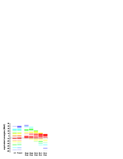
Figure 1: (color online) The neutron equivalent single-particle energies (84) for $N$=70 and $Z$=50 obtained in the HFB+LN method (first spectrum), HFB+VAPNP method using the average quasiparticle energies $E_{n}$ (second spectrum) (85), and by using the ‘quasiparticle’ energies $E^{N}_{k}$ calculated in the HFB+VAPNP method for different values of the intrinsic neutron $\bar{N}$ and proton $\bar{Z}$ numbers (the remaining five spectra). The dashed line indicates the position of the LN Fermi energy $\lambda$.

The results of such a procedure are illustrated in Fig. 1. The left-most spectrum shows the neutron equivalent energies obtained within the LN method applied to $N$=70 and $Z$=50, and the dashed line shows the position of the corresponding LN neutron Fermi energy $\lambda$. For $\bar{e}_{n}<0$, this spectrum is very similar to the HF bound single-particle energies of this nucleus. Our method, based on the average quasiparticle energies (85), gives almost identical negative equivalent energies and quite similar positive ones. In particular, for highly positive equivalent energies, in the region of the cut-off energy $\epsilon_{\text{cut}}=$ 60 MeV, similar continuum quasiparticle states appear in both methods; this guarantees the correct application of the cut-off procedure. The five equivalent spectra shown on the right hand side of Fig. 1 were calculated directly from the unphysical ‘quasiparticle’ energies $E^{N}_{n}$ obtained for several selected values of the intrinsic particle numbers $\bar{N}$ and $\bar{Z}$. It is obvious that these spectra (even at $\bar{N}$=70 and $\bar{Z}$=50) bear no resemblance to the real single-particle spectra and cannot be used to define the cut-off procedure.

V Sample results

To illustrate the Skyrme HFB+VAPNP procedure, we carried out calculations for the complete chain of calcium isotopes, from the proton drip line to the neutron drip line, and for the chain of tin isotopes with $70\leq{N}\leq 90$. We used the Sly4 Skyrme force parameterization [Cha98] and the mixed delta pairing [Dob01c] ; [Dob02c] . The calculations were performed in the basis of 20 major HO shells. We took $L$=13 gauge-angle points, and this practically ensures exact projection for all considered nuclei. We have found that the HFB+VAPNP procedure is just $L$-times slower compared to the PLN method.

In our standard HFB calculations [Dob96] ; [Dob01a] , the strength of the pairing force (assumed identical for protons and neutrons) is usually adjusted at a given cut-off energy $\epsilon_{\text{cut}}=60$ MeV to the experimental value of the average neutron gap $\tilde{\Delta}_{n}$=1.245 MeV in ¹²⁰Sn. In the present study, we used this procedure to fix the pairing force for all LN and PLN calculations. However, it is well known that the PNP method requires another strength of the pairing force. Unfortunately, the average pairing gap $\tilde{\Delta}_{n}$ is not defined within the VAPNP approach, and the standard procedure for adjusting the pairing strength is no longer applicable. In this study, we adjusted the VAPNP pairing strength to the total energy of the ⁴⁴Ca nucleus calculated in HFB+PLN. A much more consistent way of fitting the pairing strength should be based on calculating the mass differences of the odd-mass and even-even nuclei, all obtained within the VAPNP method. We intend to adopt such a procedure in future applications.

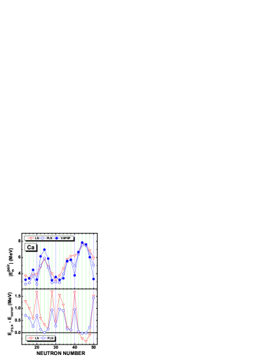
Figure 2: Comparison between the LN, PLN, and VAPNP results for the chain of Ca isotopes. The upper panel shows the neutron pairing energies while the lower panel shows the total LN and PLN energies relative to the VAPNP values.

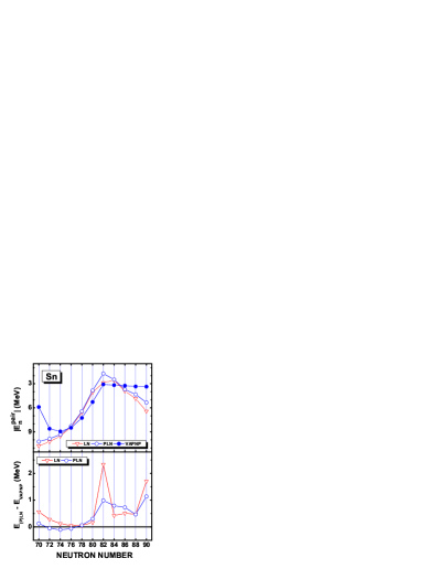
Figure 3: Similar to Fig. 2, except for the chain of Sn isotopes.

A measure of pairing correlations in a nucleus is the particle-particle energy (pairing energy) given by the second term in Eq. (44). The energy of proton pairing correlations is about 2–3 MeV and it changes smoothly with $N$ along the isotopic chains. On the other hand, the neutron pairing is significantly affected by the shell structure. As seen in Figs. 2 and 3, upper panels, the neutron pairing energies obtained within the LN, PLN, and VAPNP methods (and with pairing strengths adjusted as described above) are quite similar to one another.

The lower panels of Figs. 2 and 3 show differences between the total energies obtained in the LN and PLN methods and those obtained in VAPNP. The LN or PLN results are fairly close to VAPNP for mid-shell nuclei, where the neutron pairing correlations are large and static in character. Near closed shells, pairing is dynamic in nature, and the LN/PLN results deviate from those obtained in VAPNP. For open-shell nuclei, the PLN approximation is particularly good; in the calcium isotopes, the deviations from the HFB+VAPNP method usually do not exceed 250 keV. For the closed-shell nuclei, on the other hand, the LN method is not appropriate [Dob93] ; [Val00] ; [Ang02] , and the energy differences increase to more than 1 MeV. Figures 2 and 3 also show that the PLN method always leads to a considerable improvement over LN, often reducing the deviation of the total energy with respect to VAPNP by about 1 MeV.

As suggested in Refs. [Dob93] ; [Mag93] , one can further improve the PLN approximation around magic nuclei by applying the PNP to the LN solutions obtained in the neighboring nuclei. This procedure is illustrated in Figs. 4 and 5 for the magic nuclei ⁴⁸Ca and ¹³²Sn, respectively. It is seen that while the projection from ⁴⁶Ca nicely reproduces the VAPNP result in ⁴⁸Ca, the approximation fails when projecting from ⁵⁰Ca. Similarly, projection from the LN solution in ¹³⁰Sn (¹³⁴Sn) gives a better (worse) result than the projection of the LN solution obtained in ¹³²Sn. We observe a similar pattern of results in other cases near closed shells; however, the improvement gained by projecting from isotopes below closed shells is not sufficient to replace the full VAPNP calculations at closed shells.

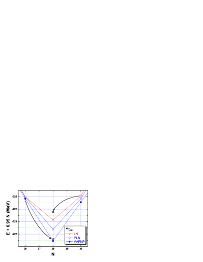
Figure 4: The total binding energy (with respect to a linear reference) as a function of $N$ for even-even nuclei around ⁴⁸Ca, calculated in the LN, PLN and VAPNP methods. Crosses indicate the PLN results for ⁴⁸Ca obtained by projecting from the LN solutions in neighboring nuclei ⁴⁶Ca and ⁵⁰Ca as indicated by arrows.

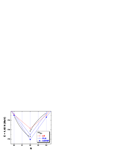
Figure 5: Similar to Fig. 4, except for nuclei near ¹³²Sn.

In order to discuss the quality of prescription to calculate the LN parameter $\lambda_{2}$ presented in Sec. III.2, we have repeated all our LN and PLN calculations with the effective pairing strengths $G^{\prime}_{\text{eff}}=\alpha G_{\text{eff}}$ scaled by factors of $\alpha$=0.9 or 1.1 with respect to those given by Eq. (47). In this way, we tested whether our results are sensitive to this phenomenological prescription. The results obtained for the chains of Ca and Sn isotopes are shown in Fig. 6. While the LN energies (45) uniformly depend on the scaling factor $\alpha$, the PLN energies are almost independent of the scaling factor. This shows that the PNP components of the LN states weakly depend on $\lambda_{2}$ and can be obtained without paying too much attention to the way in which $\lambda_{2}$ is calculated. A rough estimate given by our phenomenological prescription is good enough to obtain reliable PLN results. On the other hand, deviations between the LN/PLN and VAPNP energies depend mostly on the local shell structure and visibly cannot be corrected by modifications of the prescription used to calculate $\lambda_{2}$. In large part, these deviations stem from the inapplicability of the LN/PLN method to closed-shell nuclei, where the total energy in function of particle number cannot be well approximated by the quadratic Kamlah expansion. Altogether, we conclude that the PLN method gives a fair approximation of the full VAPNP results, but fails in reproducing detailed values, especially near closed shells.

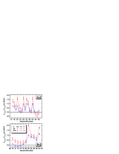
Figure 6: Total LN and PLN energies relative to the VAPNP values, calculated in the Ca (upper panel) and Sn (lower panel) isotopes with the effective pairing strengths scaled by a factor $\alpha$.

VI Summary and discussion

In this study, the variation after particle-number projection is discussed in the context of the nuclear density functional theory. Specifically, we implement for the first time the self-consistent Skyrme HFB+VAPNP formalism. We demonstrate that the particle-number conserving HFB equations with Skyrme functionals can be simply obtained from the standard Skyrme HFB equations in coordinate space by replacing the intrinsic densities and currents by their gauge-angle-dependent counterparts.

The calculations are carried for the Ca and Sn isotope chains. The VAPNP results are compared with those obtained with the LN and PLN methods. We demonstrate that the pathological behavior of LN and PLN methods around closed-shell nuclei can be partly cured by performing particle-number projection from neighboring open-shell systems. This result is important in the context of large-scale microscopic mass calculations, such as those of Ref. [Sam04] .

The restoration of broken symmetries in the density functional theory causes a number of fundamental questions, mainly related to the density dependence of the underlying interaction and to the different treatment of particle-hole and particle-particle channels [Ang01a] ; [Sto04c] . These questions and problems will be discussed in detail in a forthcoming paper.

References

(1)
A. Bohr and B.R. Mottelson, Nuclear Structure (Benjamin, New York,
1975), Vol. II.
(2)
P. Ring and P. Schuck, The Nuclear Many-Body Problem (Springer-Verlag,
Berlin, 1980).
(3)
D.M. Brink and R.A. Broglia, Nuclear Superfluidity: Pairing In Finite
Systems (Cambridge Univ. Press, Cambridge, 2005).
(4)
D.J. Dean and M. Hjorth-Jensen, Rev. Mod. Phys. 75, 607 (2003).
(5)
J. Dobaczewski and W. Nazarewicz, Phil. Trans. R. Soc. Lond. A 356, 2007
(1998).
(6)
J. Bardeen, L.N. Cooper, and J.R. Schrieffer, Phys. Rev. 108, 1175
(1957).
(7)
H. Flocard and N. Onishi, Ann. Phys. (NY) 254, 275 (1997).
(8)
A. Kamlah, Z. Phys. 216, 52 (1968).
(9)
D.C. Zheng, D.W.L. Sprung, and H. Flocard, Phys. Rev. C 46, 1355 (1992).
(10)
H.J. Lipkin, Ann. of Phys., 9, 272 (1960).
(11)
Y. Nogami, Phys. Rev. 134 (1964) B313.
(12)
B. Gall, P. Bonche, J. Dobaczewski, H. Flocard, and P.-H. Heenen, Z. Phys.
A 348, 183 (1994).
(13)
P.-G. Reinhard, W. Nazarewicz, M. Bender, and J. Maruhn, Phys. Rev.
C 53, 2776 (1996).
(14)
S. Ćwiok, J. Dobaczewski, P.-H. Heenen, P. Magierski, and W. Nazarewicz,
Nucl. Phys. A 611, 211 (1996).
(15)
A. Valor, J.L. Egido, and L.M. Robledo, Phys. Lett. B 392, 249 (1997).
(16)
A. Valor, J.L. Egido, and L.M. Robledo, Nucl. Phys. A 665, 46 (2000).
(17)
M. Bender, K. Rutz, P.-G. Reinhard, and J.A. Maruhn, Eur. Phys. Jour. A 8, 59 (2000).
(18)
M.V. Stoitsov, J. Dobaczewski, W. Nazarewicz, S. Pittel, and D.J. Dean, Phys.
Rev. C 68, 054312 (2003).
(19)
M. Anguiano, J.L. Egido, and L.M. Robledo, Phys. Lett. B 545, 62
(2002).
(20)
J. Dobaczewski and W. Nazarewicz, Phys. Rev. C 47, 2418 (1993).
(21)
P. Magierski, S. Ćwiok, J. Dobaczewski, and W. Nazarewicz, Phys. Rev.
C 48, 1686 (1993).
(22)
M. Samyn, S. Goriely, M. Bender, and J.M. Pearson, Phys. Rev. C 70,
044309 (2004).
(23)
K. Dietrich, H.J. Mang, and J.H. Pradal, Phys. Rev. B 135, 22 (1964).
(24)
K.W. Schmid and F. Grümmer, Rep. Progr. Phys. 50, 731 (1987).
(25)
J.A. Sheikh and P. Ring, Nucl. Phys. A 665, 71 (2000).
(26)
M. Anguiano, J.L. Egido, and L.M. Robledo, Nucl. Phys. A 696, 467
(2001).
(27)
J.A. Sheikh, P. Ring, E. Lopes, and R. Rossignoli, Phys. Rev. C 66,
044318 (2002).
(28)
M.V. Stoitsov, J. Dobaczewski, W. Nazarewicz, and P. Ring, Comput. Phys.
Commun. 167, 43 (2005).
(29)
M.V. Stoitsov, J. Dobaczewski, W. Nazarewicz, and J. Terasaki, Eur. Phys. J.
A 25, s01, 567 (2005).
(30)
A. Bulgac, Preprint FT-194-1980, Central Institute of Physics, Bucharest,
1980; nucl-th/9907088.
(31)
J. Dobaczewski, H. Flocard and J. Treiner, Nucl. Phys. A 422, 103
(1984).
(32)
E. Perlińska, S.G. Rohoziński, J. Dobaczewski, and W. Nazarewicz, Phys.
Rev. C 69, 014316 (2004).
(33)
Y.M. Engel, D.M. Brink, K. Goeke, S.J. Krieger, and D. Vautherin, Nucl. Phys.
A 249, 215 (1975).
(34)
K. Hara, S. Iwasaki, and K. Tanabe, Nucl. Phys. A 332 69 (1979).
(35)
J. Dobaczewski, W. Nazarewicz, T.R. Werner, J.-F. Berger, C.R. Chinn, and J.
Dechargé, Phys. Rev. C 53, 2809 (1996).
(36)
J. Dobaczewski, W. Nazarewicz, and P.-G. Reinhard, Nucl. Phys. A 693, 361
(2001).
(37)
E. Chabanat, P. Bonche, P. Haensel, J. Meyer, and F. Schaeffer, Nucl. Phys.
A 635, 231 (1998).
(38)
J. Dobaczewski, W. Nazarewicz, and M.V. Stoitsov, Proceedings of the NATO
Advanced Research Workshop The Nuclear Many-Body Problem 2001, Brijuni,
Croatia, June 2-5, 2001, eds. W. Nazarewicz and D. Vretenar (Kluwer,
Dordrecht, 2002), p. 181.
(39)
J. Dobaczewski, W. Nazarewicz, and M. V. Stoitsov, Eur. Phys. J. A 15,
21 (2002).
(40)
A. Valor, J.L. Egido, and L.M. Robledo, Nucl.Phys. A 671, 189 (2000).
(41)
M. Stoitsov, J. Dobaczewski, W. Nazarewicz, P.G. Reinhard, and J.Terasaki,
Proc. 8th International Spring Seminar on Nuclear Physics, Key Topics in
Nuclear Structure, Paestum, Italy 2004; ed. by Aldo Covello (World
Scientific, Singapore), p. 167.