The continuum description with pseudo-state wave functions

Abstract

Benchmark calculations are performed aiming to test the use of two different pseudo-state bases on the Multiple Scattering expansion of the total Transition amplitude scattering framework. Calculated differential cross sections for $p$-⁶He inelastic scattering at 717 MeV/u show a good agreement between the observables calculated in the two bases. This result gives extra confidence on the pseudo-state representation of continuum states to describe inelastic/breakup scattering.

Inelastic scattering at intermediate energies can be a useful tool to study multipole excitations of Borromean nuclei (like ¹¹Li and ⁶He). Due to their loosely bound nature, to properly understand and interpret such reactions, it is crucial to take into account the few-body degrees of freedom. At high energies, the Multiple Scattering expansion of the total Transition amplitude (MST) is a convenient framework that has already been applied to analyze such reactions for elastic Crespo and Thompson (2001); Crespo et al. (2006a) as well as for inelastic Crespo et al. (2002, 2006b) scattering. In the latter case, the method can take into account spin excitations that occur when scattering from a spin target such as a proton. In these calculations, it is formal and numerically advantageous to represent the continuum states in terms of a basis of square-integrable functions, also known as pseudo-states (PS). Unlike the true scattering states, the PS vanish at large distances and hence the method will be only useful if the calculated observables are not sensitive to the asymptotic region. Moreover, calculations performed with different families of states, should converge to the same results, provide that enough states are included, and that the basis is complete within the radial region which is relevant for the process under study.

Guided by this motivation, in this Brief Report we present benchmark calculations of proton inelastic scattering from ⁶He within the MST scattering framework making use of two different PS bases to describe the ⁶He continuum. We aim to check to what extent the calculated breakup observables depend on the choice of the PS functions.

For a Borromean system, like ⁶He, the wave function for a total angular momentum $J$ (with projection $M$) and energy $\epsilon$, $\varphi^{JM}_{\epsilon}$, can be expressed in terms of the Jacobi coordinates $\vec{r}$ (the relative coordinate between the valence nucleons) and $\vec{R}$ (the relative coordinate from the center of mass of the neutron pair to the core).

It is also convenient to introduce a set of hyperspherical coordinates: the hyperradius $\rho$ and five hyperspherical polar angles $\Omega_{5}=\{\alpha,\theta_{x},\phi_{x},\theta_{y},\phi_{y}\}$. The former is defined as $\rho=\sqrt{x^{2}+y^{2}}$ with scaled coordinates $\vec{x}=2^{-1/2}\vec{r}$ and $\vec{y}=(2/\sqrt{3})\vec{R}$. The angle $\alpha=\arctan(x/y)$ is the hyperangle and $\theta_{x},\phi_{x},\theta_{y},\phi_{y}$ the angles associated with the unit spatial vectors $\hat{x}$ and $\hat{y}$.

Within the PS method, the eigenstates $\varphi^{JM}_{\epsilon}(\vec{r},\vec{R})$ are obtained by diagonalization of the Hamiltonian in a basis of normalizable states. These states are conveniently expanded in a basis of Hyperspherical Harmonics of the form

$$\psi^{JM}_{n\beta}(\vec{r},\vec{R})=R_{n\beta}(\rho)\Upsilon_{\beta}^{JM}(\Omega_{5})~{}~{},$$ (1)

where ${\Upsilon}_{\beta}^{JM}(\Omega_{5})$ is the generalized angle-spin basis Danilin et al. (1998)

$${\Upsilon}_{\beta}^{JM}(\Omega_{5})=\left\{{\cal Y}_{{\cal K}\ell_{x}\ell_{y}L}(\Omega_{5})\otimes\left[\chi_{s_{2}}\otimes\chi_{s_{3}}\right]_{S}\right\}_{JM}~{}~{}$$ (2)

with $\chi_{s_{i}}$ the neutron spin functions and ${\cal Y}_{{\cal K}\ell_{x}\ell_{y}L}(\Omega_{5})$ the hyperspherical harmonics,

$${\cal Y}_{{\cal K}\ell_{x}\ell_{y}LM_{L}}(\Omega_{5})=\psi_{{\cal K}\ell_{x}\ell_{y}}(\alpha)\left[Y_{\ell_{x}}(\hat{x})\otimes Y_{\ell_{y}}(\hat{y})\right]_{LM_{L}}~{}.$$ (3)

The functions $\psi_{{\cal K}\ell_{x}\ell_{y}}(\alpha)$ have an explicit form in terms of Jacobi polynomials of the hyperangle $\alpha$ Danilin et al. (1998). The set of quantum numbers $\beta=\{{\cal K}\ell_{x}\ell_{y}LS\}$ defines a channel, with $\ell_{x}$ and $\ell_{y}$ the orbital angular momenta associated with the Jacobi coordinates $\vec{x}$ and $\vec{y}$, ${\cal K}=\ell_{x}+\ell_{y}+2\nu$ ($\nu$=0,1,2, $\ldots$) the hyperangular momentum, $\vec{L}=\vec{\ell}_{x}+\vec{\ell}_{y}$ the total orbital angular momentum and $S$ the spin of the particles related by the coordinate $\vec{x}$. In Eq. (1), $R_{n\beta}(\rho)$ are the hyperradial functions and $n$ is an index that labels the basis states within a given channel $\beta$. These functions are orthogonalized such that

$$\int_{0}^{\infty}d\rho\,\rho^{5}R_{n\beta}(\rho)R_{n^{\prime}\beta}(\rho)=\delta_{nn^{\prime}}\ .$$ (4)

The aim of the present work is to compare two different choices for the functions $R_{n\beta}(\rho)$ in the calculation of breakup observables within the MST scattering framework. First, we consider the Gauss-Laguerre (GL) basis Thompson et al. (2004), whose hyperradial part, $R_{n}^{GL}(\rho)$, is given by

$$R_{n}^{GL}(\rho)={\rho_{0}}^{-3}[n!/(n+5)!]^{1/2}L_{n}^{5}(z)\exp(-z/2)\,,$$ (5)

with $z=\rho/\rho_{0}$, $L_{n}^{5}$ the generalized Laguerre polynomials, and $\rho_{0}$ a parameter that sets the radial scale of the basis.

The second choice is the Transformed Harmonic Oscillator (THO) basis, recently introduced in Ref. Rodríguez-Gallardo et al. (2005) for a three-body system. The THO method is based on the idea of transforming the bound ground state wave function of the system into the ground state wave function of the Harmonic Oscillator (HO), defining a Local Scale Transformation (LST). The ground state wave function can be written as a linear combination of the basis functions (1),

$$\varphi^{J_{0}M_{0}}_{0}(\vec{r},\vec{R})=\sum_{\beta}R_{\beta}^{\epsilon_{0}}(\rho)\Upsilon_{\beta}^{J_{0}M}(\Omega_{5})~{}~{},$$ (6)

where we have introduced the abbreviated notation $\varphi^{J_{0}M_{0}}_{0}\equiv\varphi^{J_{0}M_{0}}_{\epsilon_{0}}$. Then, the equation that defines the LST for each channel $\beta$ is

$$\int_{0}^{\rho}d\rho^{\prime}\rho^{\prime 5}|R^{{\epsilon_{0}}}_{\beta}(\rho^{\prime})|^{2}=\int_{0}^{s}ds^{\prime}s^{\prime 5}|R^{HO}_{0{\cal K}}(s^{\prime})|^{2},$$ (7)

where $R^{HO}_{0{\cal K}}(s)$ is the hyperradial part of the HO ground state for the hyperangular momentum ${\cal K}$. Then, the THO basis is constructed for each channel applying the LST, $s_{\beta}(\rho)$, to the HO basis

$$R^{THO}_{n\beta}(\rho)=R^{{\epsilon_{0}}}_{\beta}(\rho)L_{n}^{{\cal K}+2}\left(s^{2}_{\beta}(\rho)\right),$$ (8)

where $L_{n}^{{\cal K}+2}$ are generalized Laguerre polynomials of degree $n$. For channels not included in the ground state, information from one of the known (ground state) channels with the closest quantum labels to the channel of interest is used to construct the LST, as explained in Ref. Rodríguez-Gallardo et al. (2005).

Neither the GL nor the THO functions are eigenstates of the Hamiltonian, but they provide a complete and orthonormal set in which the Hamiltonian can be diagonalized. For this purpose, the basis is truncated by setting a maximum value of the index $n$ ($n=0,\ldots,N$) as well as a maximum hyperangular momentum ${\cal K}_{\mathrm{max}}$. Upon diagonalization in the truncated basis, the eigenstates are obtained as

$$\varphi_{\epsilon_{i}}^{JM}(\vec{r},\vec{R})=\sum_{n\beta}C_{n\beta}^{J\epsilon_{i}}\psi_{n\beta}^{JM}(\vec{r},\vec{R}).$$ (9)

where $\{\epsilon_{i}\}$ are their associated eigenvalues.

From the derivation above, it becomes apparent that the GL basis is obtained in a more straightforward way than the THO basis. However, the latter has some appealing properties that could make it more suitable in some situations. In particular, the THO basis has the advantage of being constructed from the ground state wave function of the system. Thus, when we diagonalize the Hamiltonian in a finite THO basis, the ground state is recovered for any size of the basis. By contrast, in the GL representation a large basis may be required to obtain a good description of the ground state. Also, note that the hyperradial part of the GL basis is the same for all the channels $\beta$ while in the THO basis a different hyperradial part is calculated for each channel, with the correct behavior at the origin ($\rho^{{\cal K}}$).

For a meaningful comparison between the two bases, we use the same three-body Hamiltonian to generate the GL and THO eigenstates for ⁶He. In particular, we use the n-n potential of Gogny, Pires and Tourreil Gogny et al. (1970) with spin-orbit and tensor components and we take the $n$-⁴He potential from Bang and Gignoux (1979). Besides the pairwise interactions, an effective three-body potential is included, with matrix elements of the form Danilin et al. (1998)

$$V^{\rm 3B}_{\beta^{\prime}\beta}(\rho)=\frac{\delta_{\beta^{\prime}\beta}V^{\rm 3B}_{J}}{1+(\rho/5)^{3}}~{}~{}.$$ (10)

The $J$=0 strength of this effective potential is tuned to reproduce the experimental three-body separation energy and the $J>0$ strength is adjusted to obtain the $2^{+}_{1}$ resonance at the experimental energy.

We now consider the scattering process of ⁶He, originally in its ground state, $|\varphi_{0}^{J_{0}M_{0}}\rangle$, to a final continuum state $|\varphi_{\epsilon}^{JM}\rangle$, at excitation energy $\epsilon$ and with total angular momentum $J$ (projection $M$), by means of its interaction with a proton, with initial (final) linear momentum $\vec{k}_{1}$ ($\vec{k}\,^{\prime}_{1}$) in the nucleon-nucleus center-of-mass frame and spin $S_{1}=1/2$ with projection $\sigma$ (${\sigma}^{\prime}$).

The double differential cross section for this process can be formally expressed as

$$\frac{d^{2}\sigma_{JJ_{0}}}{d\Omega d\epsilon} = \frac{1}{(\widehat{S_{1}})^{2}}\frac{1}{(\widehat{J_{0}})^{2}}\left[\frac{\hbar^{2}}{4\pi^{2}\mu_{NA}}\right]^{2}$$

$$\times \sum_{\sigma{\sigma}^{\prime}}\sum_{MM_{0}}|\langle\vec{k}^{\prime}_{1}\chi_{S_{1}}^{{\sigma}^{\prime}};\varphi_{\epsilon}^{JM}|{\cal T}|\vec{k}_{1}\chi_{S_{1}}^{\sigma};\varphi_{0}^{J_{0}M_{0}}\rangle|^{2}$$

where ${\cal T}$ denotes the transition amplitude operator Joachain (1987). This operator can be expressed as a multiple expansion series in the transition amplitudes $\hat{t}_{\cal I}$ for proton scattering from each projectile sub-system ${\cal I}$ Watson (1957). At high energies and for small momentum transfers, this expansion is expected to converge quickly. If only the leading term of the series is retained, the single scattering approximation (SSA) is obtained Crespo and Johnson (1999); Crespo et al. (2002):

$${\cal T}^{SSA}=\sum_{{\cal I}=2}^{4}\hat{t}_{1{\cal I}}$$ (12)

with ${\cal I}$=2,3 for the halo neutrons, and ${\cal I}$=4 for the core. The proton - ${\cal I}$ subsystem transition amplitude satisfies the Lippmann-Schwinger equation

$$\hat{t}_{1{\cal I}}=v_{1{\cal I}}+v_{1{\cal I}}G_{0}\hat{t}_{1{\cal I}}~{}~{},$$ (13)

with $v_{1{\cal I}}$ the interaction between the nucleon and ${\cal I}$ subsystem. Within the impulse approximation, the propagator $G_{0}=\left(E^{+}-K\right)^{-1}$ contains the kinetic energy operators of the proton and all the projectile subsystems. Here $E$ is the kinetic energy, $E=\frac{\hbar^{2}k_{1}^{2}}{2\mu_{NA}}$ in the overall center of mass frame, and $\mu_{NA}$ is the proton-projectile reduced mass.

Within the PS method, the scattering states $\varphi_{\epsilon}^{JM}$ in Eq. (The continuum description with pseudo-state wave functions) are approximated by the pseudo-states $\varphi_{\epsilon_{i}}^{JM}$. Hence, the double differential cross section (The continuum description with pseudo-state wave functions) becomes a single differential cross section for each pseudo-state,

$$\frac{d\sigma_{JJ_{0}}^{i}}{d\Omega} = \frac{1}{(\widehat{S_{1}})^{2}}\frac{1}{(\widehat{J_{0}})^{2}}\left[\frac{\hbar^{2}}{4\pi^{2}\mu_{NA}}\right]^{2}$$

$$\times \sum_{\sigma{\sigma}^{\prime}}\sum_{MM_{0}}|\langle\vec{k}^{\prime}_{1}\chi_{S_{1}}^{{\sigma}^{\prime}};\varphi_{\epsilon_{i}}^{JM}|\sum_{{\cal I}=2}^{4}\hat{t}_{1{\cal I}}|\vec{k}_{1}\chi_{S_{1}}^{\sigma};\varphi_{0}^{J_{0}M_{0}}\rangle|^{2}$$

where we have replaced the ${\cal T}$ matrix operator by its single scattering approximation. Making use of the impulse approximation Crespo et al. (2006a), the matrix elements for the scattering for each constituent can be further simplified, leading to the following factorized form for the scattering from one valence nucleon (${\cal I}$=2):

$$\langle\vec{k}^{\prime}_{1}\chi_{S_{1}}^{{\sigma}^{\prime}};\varphi_{{\epsilon}_{i}}^{JM}|\hat{t}_{12}|\vec{k}_{1}\chi_{S_{1}}^{\sigma};\varphi_{0}^{J_{0}M_{0}}\rangle=$$

$$\sum_{b\beta}{t}_{[b\beta{\cal S}_{p}{\cal S}^{\prime}_{p}]}(\omega_{12},{\Delta})\times\rho_{[b\beta;{\cal S}_{T}{\cal S}^{\prime}_{T}{\epsilon}_{i}]}\left(\frac{m_{3}}{M_{23}}\vec{\Delta},\frac{m_{4}}{M_{234}}\vec{\Delta}\right)$$

with $M_{23}=m_{2}+m_{3},M_{234}=m_{2}+m_{3}+m_{4}$ and where we have introduced the momentum transfer $\vec{\Delta}=\vec{k}\,^{\prime}_{1}-\vec{k}_{1}$ and the energy parameter $\omega_{12}$ Crespo et al. (2006a) and where ${\cal S}_{p}=\{S_{1}\sigma\}$ (${\cal S}^{\prime}_{p}=\{S_{1}\sigma^{\prime}\}$) are the incoming (outgoing) spin of the nucleon and its projection and, ${\cal S}_{T}=\{J_{0}M_{0}\}$ (${\cal S}^{\prime}_{T}=\{JM\}$) the initial (final) total spin of the halo valence pair. The amplitude ${t}_{[b\beta{\cal S}_{p}{\cal S}^{\prime}_{p}]}$ is given in terms of the tensor components of the nucleon-nucleon transition amplitude Crespo et al. (2006a); Crespo and Moro (2002). The transition density form factors, $\rho_{[b\beta;{\cal S}_{T}{\cal S}^{\prime}_{T}{\epsilon}_{i}]}$, depend exclusively on the structure of the composite system. Its explicit expression as a function of the hyperradial parts of the wave functions of the initial and final states, can be found in Crespo et al. (2006a).

The scattering from the core, assumed here as spinless, can equivalently be written as:

$$\langle\vec{k}^{\prime}_{1}\chi_{S_{1}}^{{\sigma}^{\prime}};\varphi_{{\epsilon}_{i}}^{JM}|\hat{t}_{14}|\vec{k}_{1}\chi_{S_{1}}^{\sigma};\varphi_{0}^{J_{0}M_{0}}\rangle=$$

$${t}_{[00{\cal S}_{p}{\cal S}^{\prime}_{p}]}(\omega_{14},{\Delta})\times\rho_{[00;{\cal S}_{T}{\cal S}^{\prime}_{T}{\epsilon}_{i}]}\left(0,\frac{M_{23}}{M_{234}}\vec{\Delta}\right)$$ (16)

where, as before, $\omega_{14}$ is the appropriate energy parameter Crespo et al. (2006a). The angular differential cross section for ⁶He inelastic scattering (breakup) is then obtained by summing all excited states contributions,

$$\frac{d\sigma^{inel}_{JJ_{0}}}{d\Omega} = \sum_{{\epsilon}_{i}}^{{\epsilon}_{i}^{\rm max}}\frac{d\sigma^{i}_{JJ_{0}}}{d\Omega}\,.$$ (17)

For the evaluation of Eqs. (The continuum description with pseudo-state wave functions) and (The continuum description with pseudo-state wave functions) one needs the (free) transition amplitudes for proton scattering from the valence nucleons and the core. For the former, we used the NN Paris interaction. The transition amplitude for the $\alpha$ core was generated from a phenomenological optical potential, of Woods Saxon form, with parameters obtained by fitting existing data for the elastic scattering of $p+^{4}$He at $E_{\rm p}=700$ and 800 MeV, as detailed in Ref. Crespo et al. (2006a).

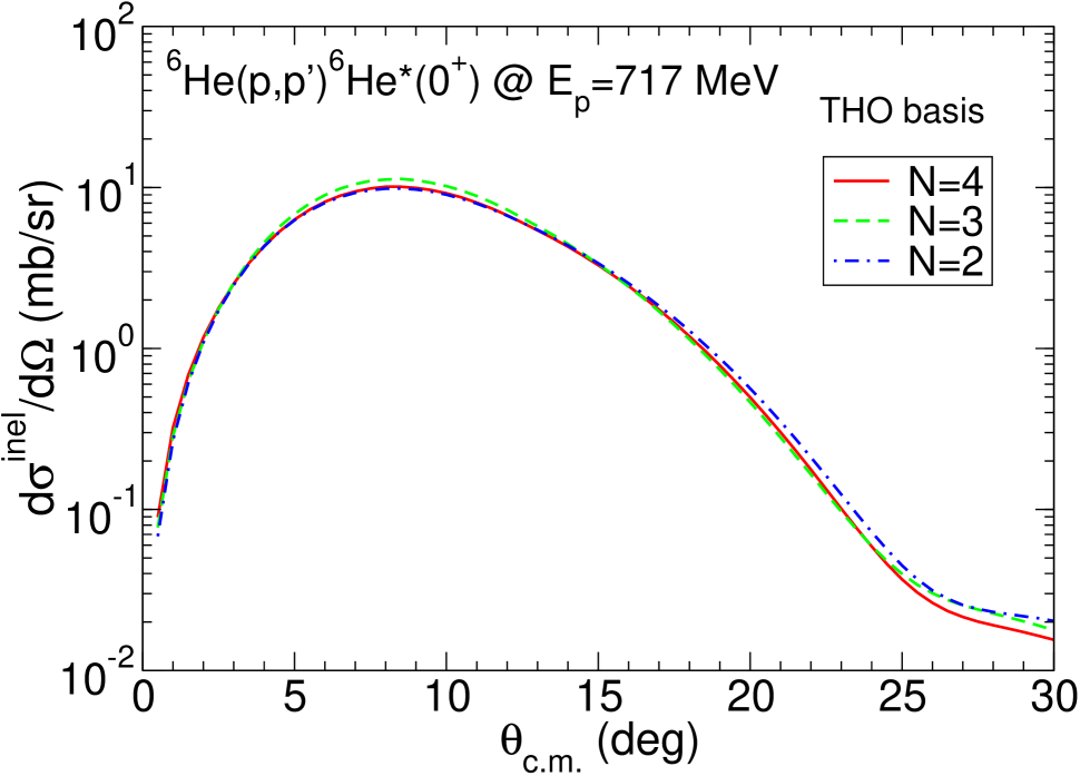
Figure 1: (Color online) Angular differential cross section for the breakup of ⁶He on protons at 717 MeV per nucleon, leading to $J^{\pi}=0^{+}$ continuum states of the ⁶He nucleus. The three lines represent the calculation with the THO basis, for several values of $N$ (indicated by the labels). Each curve includes the contribution from eigeinstates up to 10 MeV in excitation energy, according to Eq. (17).

We first study the convergence of the breakup observables with respect to the basis size. For this purpose, we consider the THO basis, truncated at different values of $N$. The maximum hyperangular momentum was set to ${\cal K}_{\mathrm{max}}=20$. This yields the three-body force parameters $V_{0}^{\rm 3B}=-2.4$ MeV, for $J=0$, and $V_{J}^{\rm 3B}=-0.85$ MeV, for $J>0$.

In Fig. 1 we show the angular distribution of the calculated inelastic differential cross sections. For simplicity, only the $J^{\pi}=0^{+}$ continuum is included, and the Coulomb interaction between the proton and the $\alpha$ core is ignored. The three lines represent the SSA calculation for different values of the basis size, according to the choice of the parameter $N$. The three cases are in almost perfect agreement, indicating that in this reaction the convergence with the basis size is very fast.

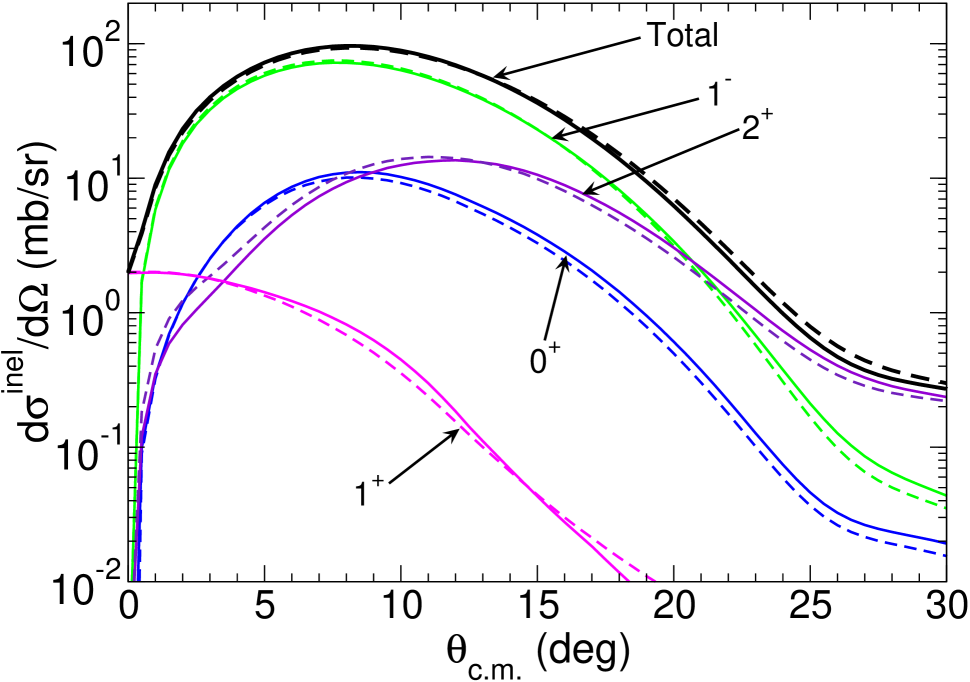
Figure 2: (Color online) Calculated contributions for breakup differential cross section leading to final states with $J^{\pi}=0^{+},1^{-},1^{+}$ and $2^{+}$, using the SSA approximation. Solid and dashed lines refer to the GL and THO basis, respectively.

Next, we study the dependence of the breakup observables on the choice of the basis, by comparing the calculations in the GL and THO representations. As before, the maximum hyperangular momentum was set to ${\cal K}_{\mathrm{max}}=20$, and only eigenstates below 10 MeV are considered. The index $n$ was truncated to $N=20$ and $N=4$ for the GL and THO bases, respectively. With this model space, the number of pseudo-states in the GL (THO) basis is: 31 (30) for $0^{+}$, 63 (86) for $1^{-}$, 53 (49) for $1^{+}$ and 79 (81) for $2^{+}$. For the GL basis, the range parameter was set to $\rho_{0}=0.25$ fm, which provides a basis that extends up to about 20 fm in the hyperradius. With these parameters, the ground state obtained after diagonalization of the Hamiltonian appears at -0.9781 MeV and -0.9549 MeV, for the GL and THO bases, respectively.

In Fig. 2 we compare the inelastic angular distributions calculated in the GL and THO bases. The separate contributions for $J^{\pi}$=$0^{+}$, $1^{-}$, $1^{+}$ and $2^{+}$ final states are also shown. As before, the Coulomb interaction is neglected. The thick lines are the incoherent sum of all these $J^{\pi}$ contributions. Solid and dashed lines correspond, respectively, to the calculations with the GL and THO bases. For each curve, the contribution of eigenstates up to $\epsilon_{\max}=10$ MeV are added incoherently, according to Eq. (17). We consider only the forward angles $\theta_{\mathrm{c.m.}}<30^{\circ}$ since the SSA is not expected to work well at large momentum transfers Crespo et al. (2006a). We see that, at these angles, the dominant contribution to the breakup cross section comes from the $1^{-}$ states, while for $\theta_{\mathrm{c.m.}}>25^{\circ}$, the $2^{+}$ excitation becomes dominant. Finally, the population of the unnatural $1^{+}$ states is almost negligible at all angles. We notice that this excitation mode requires spin-flip transitions which, according to these calculations, are very small in this reaction.

For all these contributions, the GL and THO bases provide very similar results, suggesting that the calculated observables do not depend on the choice of the continuum representation, provided that enough states are included.

In summary, in this Brief Report we have calculated proton inelastic scattering from ⁶He at 717 MeV/u, using as scattering framework the single-scattering approximation and two different pseudo-state representations of the ⁶He continuum: the GL and the THO. Provided that enough states are included, both bases predict essentially the same inelastic differential cross section. Furthermore, the studied observables converge very quickly with the size of the basis. These results support the reliability of the pseudo-state method as a useful and convenient tool to treat scattering problems dealing with continuum states. This analysis could be extended to other PS bases and reactions. Furthermore, it could be applied to other scattering frameworks, for which the PS method has been also implemented, such as the continuum discretized coupled channels (CDCC) method Moro et al. (2006); Matsumoto et al. (2004).

Acknowledgements: This work was supported by the Fundação para a Ciência e Tecnologia (Portugal) through grant No. POCTI/1999/FIS/36282, by the Acción Integrada HP2003-0121 and in the U.K. by EPSRC grant GR/M/82141. A.M.M. acknowledges a research grant by the Junta de Andalucía. We are grateful to J. Gómez-Camacho and J.M. Arias for useful discussions.

References

- Crespo and Thompson (2001) R. Crespo and I. J. Thompson, Phys. Rev. C 63, 044003 (2001).
- Crespo et al. (2006a) R. Crespo, A. M. Moro, and I. J. Thompson, Nucl. Phys. A 771, 26 (2006a).
- Crespo et al. (2002) R. Crespo, I. J. Thompson, and A. A. Korsheninnikov, Phys. Rev. C 66, 021002(R) (2002).
- Crespo et al. (2006b) R. Crespo, I. J. Thompson, and A. M. Moro, Phys. Rev. C 74, 044616 (2006b).
- Danilin et al. (1998) B. V. Danilin, I. J. Thompson, M. V. Zhukov, and J. S. Vaagen, Nucl. Phys. A632, 383 (1998).
- Thompson et al. (2004) I. Thompson, F. Nunes, and B. Danilin, Comp. Phys. Com. 161, 87 (2004).
- Rodríguez-Gallardo et al. (2005) M. Rodríguez-Gallardo, J. M. Arias, J. Gómez-Camacho, A. M. Moro, I. J. Thompson, and J. A. Tostevin, Phys. Rev. C 72, 024007 (2005).
- Gogny et al. (1970) D. Gogny, P. Pires, and R. de Tourreil, Phys. Lett. 32B, 591 (1970).
- Bang and Gignoux (1979) J. Bang and C. Gignoux, Nucl. Phys. A 313, 119 (1979).
- Joachain (1987) C. J. Joachain, Quantum collision theory (North-Holland, 1987).
- Watson (1957) K. M. Watson, Phys. Rev. 105, 1388 (1957).
- Crespo and Johnson (1999) R. Crespo and R. C. Johnson, Phys. Rev. C 60, 034007 (1999).
- Crespo and Moro (2002) R. Crespo and A. M. Moro, Phys. Rev. C 65, 054001 (2002).
- Moro et al. (2006) A. M. Moro, F. Pérez-Bernal, J. M. Arias, and J. Gómez-Camacho, Phys. Rev. C 73, 044612 (2006).
- Matsumoto et al. (2004) T. Matsumoto, E. Hiyama, K. Ogata, Y. Iseri, M. Kamimura, S. Chiba, and M. Yahiro, Phys. Rev. C 70, 061601(R) (2004).