Effective Field Theory and the Nuclear Many Body Problem

Abstract

We review many body calculations of the equation of state of dilute neutron matter in the context of effective field theories of the nucleon-nucleon interaction.

1 Introduction

One of the central problems of nuclear physics is to calculate the properties of nuclear matter starting from the two-body scattering data and the binding energies of few body bound states Bethe:1971xm ; Jackson:1984ha . The nuclear matter problem is notoriously difficult. Some of the problems that are often mentioned are

• the large short-range repulsive core in the nucleon-nucleon interaction

• the large scattering length in the ${}^{1}S_{0}$ channel, the small binding energy of the deuteron, and the small saturation density

• the need to include three (and possibly four) body forces

• the need to include non-nucleonic degrees of freedoms, such as isobars, mesons, quarks, etc.

Ever since the discovery of QCD the classic nuclear matter problem has evolved into the broader question of how the properties of nuclear matter are related to the parameters of the QCD, the QCD scale parameter and the masses of the light quarks.

Over the last couple of year much progress has been made in understanding these kinds of questions in the case of nuclear two and three-body bound states Weinberg:1990rz . Using effective field theory methods it was shown that

• the short range behavior of the nuclear force is not observable. Using the renormalization group the short distance behavior can be modified without changing low energy scattering data and binding energies Lepage:1997cs ; Bogner:2003wn .

• effective field theories can accommodate the large scattering lengths in the nucleon-nucleon system Kaplan:1998we . The scattering lengths depend sensitively on the quark masses, see Fig. 1, and the large value of $a(^{1}S_{0})$ observed in nature appears to be accidental Beane:2002xf ; Epelbaum:2002gb .

• a local three body force is necessary to renormalize the two-body force already at leading order. As a consequence, one cannot predict three-body binding energies based on two-body scattering data alone Bedaque:1998kg .

• non-nucleonic degrees of freedom, quark effects, relativistic effects etc. can be absorbed in local operators.

Effective field theories have also achieved remarkable quantitative success in describing the available nucleon-nucleon scattering data below the pion production threshold Epelbaum:2005pn ; Entem:2003ft . The long term goal is to achieve a similar qualitative and quantitative understanding of the nuclear many body problem.

In this contribution we shall study a simple limiting case of the nuclear matter problem. We shall concentrate on pure neutron matter at densities significantly below nuclear matter saturation density. The neutron-neutron scattering length is $a_{nn}=-18$ fm and the effective range is $r_{nn}=2.8$ fm. This means that there is a range of densities for which the inter-particle spacing is large compared to the effective range but small compared to the scattering length. Neutron matter in this regime exhibits interesting universal properties. We are interested in the limit $(k_{F}a_{nn})\to\infty$ and $(k_{F}r_{nn})\to 0$, where $k_{F}$ is the Fermi momentum. From dimensional analysis it is clear that the energy per particle at zero temperature has to be proportional to energy per particle of a free Fermi gas at the same density

$$\frac{E}{A}=\xi\Big{(}\frac{E}{A}\Big{)}_{0}=\xi\frac{3}{5}\Big{(}\frac{k_{F}^{2}}{2m}\Big{)}.$$ (1)

The constant $\xi$ is universal, i. e. independent of the details of the system. Similar universal constants govern the magnitude of the gap in units of the Fermi energy and the equation of state at finite temperature.

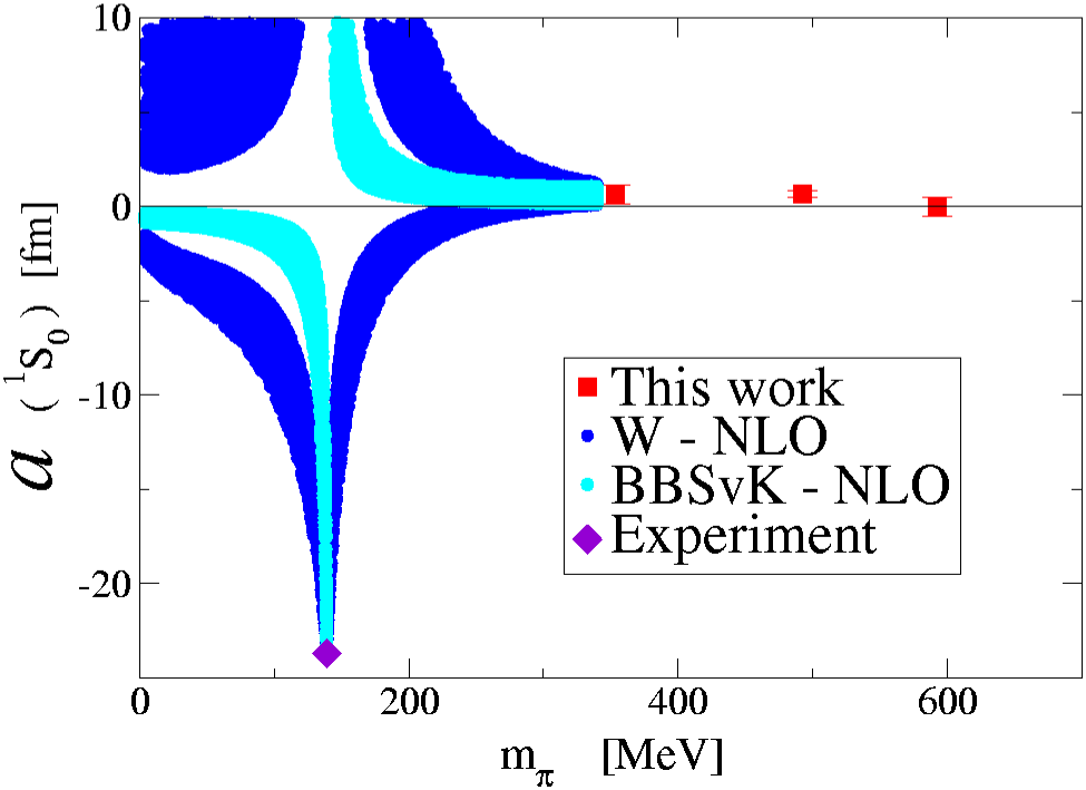
Figure 1: Quark mass dependence of the scattering length in the ${}^{1}S_{0}$ channel. The plot shows a combination of unquenched lattice QCD results (red points, from Beane et al. Beane:2006mx ) and chiral extrapolations. The experimental point is shown in purple. Two different power counting schemes were employed to constrain the quark mass dependence, the BBSvK scheme Kaplan:1998we ; Beane:2001bc and the W (Weinberg) scheme Weinberg:1990rz .

Universality also implies that the properties of this system can be studied using atoms rather than nuclei. The scattering length of certain fermionic atoms can be tuned using Feshbach resonances, see Regal:2005 for a review. A small negative scattering length corresponds to a weak attractive interaction between the atoms. This case is known as the BCS limit. As the strength of the interaction increases the scattering length becomes larger. It diverges at the point where a bound state is formed. The point $a=\infty$ is called the unitarity limit, since the scattering cross section saturates the $s$-wave unitarity bound $\sigma=4\pi/k^{2}$. On the other side of the resonance the scattering length is positive. In the BEC limit the interaction is strongly attractive and the fermions form deeply bound molecules.

2 Numerical Calculations

The calculation of the dimensionless quantity $\xi$ is a non-perturbative problem. In this section we shall describe an approach based on lattice field theory methods. The physics of the unitarity limit is captured by an effective lagrangian of point-like fermions interacting via a short-range interaction. The lagrangian is

$${\cal L}=\psi^{\dagger}\left(i\partial_{0}+\frac{\vec{\nabla}^{2}}{2m}\right)\psi-\frac{C_{0}}{2}\left(\psi^{\dagger}\psi\right)^{2}.$$ (2)

The standard strategy for dealing with the four-fermion interaction is to use a Hubbard-Stratonovich transformation. The partition function can be written as Lee:2004qd

$$Z=\int DsDcDc^{\ast}\exp\left[-S\right],$$ (3)

where $s$ is the Hubbard-Stratonovich field and $c$ is a Grassmann field. $S$ is a discretized euclidean action

$$S = \sum_{\vec{n},i}\left[e^{-\hat{\mu}\alpha_{t}}c_{i}^{\ast}(\vec{n})c_{i}(\vec{n}+\hat{0})\right.$$ (4)

$$\hskip 14.22636pt\mbox{}\left.-e^{\sqrt{-C_{0}\alpha_{t}}s(\vec{n})+\frac{C_{0}\alpha_{t}}{2}}(1-6h)c_{i}^{\ast}(\vec{n})c_{i}(\vec{n})\right]$$

$$\mbox{}-h\sum_{\vec{n},l_{s},i}\left[c_{i}^{\ast}(\vec{n})c_{i}(\vec{n}+\hat{l}_{s})+c_{i}^{\ast}(\vec{n})c_{i}(\vec{n}-\hat{l}_{s})\right]$$

$$\mbox{}+\frac{1}{2}\sum_{\vec{n}}s^{2}(\vec{n}).$$

Here $i$ labels spin and $\vec{n}$ labels lattice sites. Spatial and temporal unit vectors are denoted by $\hat{l}_{s}$ and $\hat{0}$, respectively. The temporal and spatial lattice spacings are $b_{\tau}$ and $b$. The dimensionless chemical potential is given by $\hat{\mu}=\mu b_{\tau}$. We define $\alpha_{t}$ as the ratio of the temporal and spatial lattice spacings and $h=\alpha_{t}/(2\hat{m})$. Note that for $C_{0}<0$ the action is real and standard Monte Carlo simulations are possible.

Figure 2: Equation of state of pure neutron matter at $T=4$ MeV from lattice simulations of an effective field theory. Figure taken from Lee & Schäfer Lee:2004qd . The curves labeled (fc,f1,f2) show results for a free gas on the lattice and in the continuum, the curves labeled (b1,b2) show ladder sums, and (s1,s2) are numerical results on different lattices. We also compare to the variational results of Friedman and Pandharipande (FP).

The four-fermion coupling is fixed by computing the sum of all two-particle bubbles where on the lattice. Schematically,

$$\frac{m}{4\pi a}=\frac{1}{C_{0}}+\frac{1}{2}\sum_{\vec{p}}\frac{1}{E_{\vec{p}}},$$ (5)

where the sum runs over discrete momenta on the lattice and $E_{\vec{p}}$ is the lattice dispersion relation. A detailed discussion of the lattice regularized scattering amplitude can be found in Chen:2003vy ; Beane:2003da ; Lee:2004qd . For a given scattering length $a$ the four-fermion coupling is a function of the lattice spacing. The continuum limit correspond to taking the temporal and spatial lattice spacings $b_{\tau}$, $b$ to zero

$$b_{\tau}\mu\to 0,\hskip 28.45274ptbn^{1/3}\to 0,$$ (6)

where $\mu$ is the chemical potential, $n$ is the density and $an^{1/3}$ is fixed. We performed numerical simulations at non-zero temperature and concluded that $\xi=(0.09-0.42)$. Lee studied canonical $T=0$ simulations and obtained $\xi=0.25$ Lee:2005fk . Green Function Monte Carlo calculations give $\xi=0.44$ Carlson:2003wm , and finite temperature lattice simulations have been extrapolated to $T=0$ to yield similar results Bulgac:2005pj ; Burovski:2006 .

Lattice results for the equation of state of dilute neutron matter at $T=4$ MeV are shown in Fig. 2. For comparison, we show variational results obtained by Friedman and Pandharipande using a phenomenological potential Friedman:1981qw . We observe that the lattice calculations agree very well with the variational result. The pressure is very similar that of non-interacting neutrons scaled by a factor $\sim 1/2$. The lattice calculation can be extended to higher densities by including explicit pionic degrees of freedom in the effective lagrangian Lee:2004si . In this case a mild sign problem returns, but at $T\neq 0$ this sign problem can be handled with standard methods.

3 Analytical Approaches: Large N expansion

It is clearly desirable to find a systematic analytical approach to the dilute Fermi liquid in the unitarity limit. Various possibilities have been considered, such as an expansion in the number of fermion species Furnstahl:2002gt ; Nikolic:2006 or the number of spatial dimensions Steele:2000qt ; Schafer:2005kg ; Nussinov:2004 ; Nishida:2006br .

We begin with a brief description of the large $N$ approach. The physics of the large $N$ limit depends on the symmetries of the interaction. One possibility is a $SU(N)$ symmetric interaction Furnstahl:2002gt

$${\cal L}=\frac{C_{0}}{2}\left(\psi^{\dagger}_{f}\psi_{f}\right)^{2},$$ (7)

where $f=1,\ldots,N$ is a flavor label. A smooth large $N$ limit is achieved by keeping $C_{0}N=c_{0}$ constant as $N\to\infty$. The large $N$ limit is most easily studied by introducing a Hubbard Stratonovich field $\sigma$ coupled to the density $\psi^{\dagger}_{f}\psi_{f}$. The leading contribution to the free energy comes from the free fermion term and the mean field contribution, both of which scale as $N$. Subleading $1/N$ corrections arise from particle-hole ring diagrams. The problem is that at any fixed order in the large $N$ expansion the free energy diverges as the scattering length is taken to infinity.

This problem is related to the fact that particle ladders need to be summed in the unitarity limit. This can be achieved by by considering a $Sp(2N)$ symmetric interaction of the form Nikolic:2006

$${\cal L}=\frac{G_{0}}{2}(\psi_{f}{\cal J}^{fg}\psi_{g})(\psi^{\dagger}_{h}{\cal J}^{hi}\psi^{\dagger}_{i}),$$ (8)

where ${\cal J}=(\sigma_{2})\otimes\ldots\otimes(\sigma_{2})$ and $G_{0}N=g_{0}$ constant as $N\to\infty$. This interaction can be bosonized using a difermion field $\Phi=(\psi_{f}{\cal J}^{fg}\psi_{g})/N$. At large $N$ the leading contribution corresponds to the mean field BCS approximation. The thermodynamic potential in the unitarity limit is

$$\Omega=-N\int\!\frac{d^{3}p}{(2\pi)^{3}}\left\{\sqrt{\epsilon_{p}^{2}+\Phi^{2}}-\epsilon_{p}-\frac{m\Phi^{2}}{p^{2}}\right\}$$ (9)

with $\epsilon_{p}=E_{p}-\mu$. This function can be minimized numerically. We find $\Phi_{0}=1.16\mu$ and $\xi=0.59$. Nikolic and Sachdev studied $1/N$ corrections near $T_{c}$ Nikolic:2006 . These effects are not small. They find, for example, $(\mu/T)(T_{c})=1.50+2.79/N+O(1/N^{2})$.

4 Large d expansion

Figure 3: The particle ladder diagrams shown in this figure give the leading order contribution to the ground state energy in the large $d$ limit.

Steele suggested that the many body problem of non-relativistic fermions near the unitarity limit can be studied using an expansion in $1/d$, where $d$ is the number of spatial dimensions Steele:2000qt . The main idea is that phase space factors associated with hole lines are suppressed as $d\to\infty$ so that the leading order contribution comes from 2-particle ladders, and higher order corrections correspond to the hole line expansion of Bethe and Brueckner.

Consider the effective lagrangian in equ. (2). We first study perturbative corrections to the ground state energy in $d$ spatial dimensions. The leading order correction to the energy per particle is

$$\frac{E_{1}}{A}=\frac{1}{d}\left[\frac{\Omega_{d}C_{0}k_{F}^{d-2}M}{(2\pi)^{d}}\right]\left(\frac{k_{F}^{2}}{2M}\right).$$ (10)

This expression indicates that the large $d$ limit should be taken in such a way that

$$\lambda\equiv\left[\frac{\Omega_{d}C_{0}k_{F}^{d-2}M}{d(2\pi)^{d}}\right]\stackrel{{\scriptstyle d\to\infty}}{{\longrightarrow}}{\it const}.$$ (11)

In the following we wish to study whether this limit is smooth even if the theory is non-perturbative. Consider the in medium two-particle scattering amplitude in $d$ spatial dimensions. The result is

$$\int\!\!\frac{d^{d}q}{(2\pi)^{d}}\;\frac{\theta_{q}^{+}}{k^{2}-q^{2}+i\epsilon}=f_{vac}(k)+\frac{k_{F}^{d-2}\Omega_{d}}{2(2\pi)^{d}}f_{PP}^{(d)}(\kappa,s).$$ (12)

The theta function $\theta_{q}^{+}\equiv\theta(k_{1}-k_{F})\theta(k_{2}-k_{F})$ with $\vec{k}_{1,2}=\vec{P}/2\pm\vec{k}$ requires both fermion momenta to be above the Fermi surface. The first term on the RHS is the vacuum contribution. In dimensional regularization the vacuum term is purely imaginary and does not contribute to the ground state energy. The second term is the medium contribution which depends on the scaled relative momentum $\vec{\kappa}=\vec{k}/k_{F}$ and center-of-mass momentum $\vec{s}=\vec{P}/(2k_{F})$. In the large $d$ limit we find

$$f_{PP}^{(d)}(s,\kappa)=\frac{1}{d}f_{PP}^{(0)}(s,\kappa)\left(1+O\left(\frac{1}{d}\right)\right),$$ (13)

which implies that all two-particle ladder diagrams are of the same order, see Fig. 3. The sum of all ladder diagrams can be calculated by noting that, except for the logarithmic (BCS) singularity at $s=0,\kappa=1$, the particle-particle bubble is a smooth function of the kinematic variables $s$ and $\kappa$. Hole-hole phase space, on the other hand, is strongly peaked at $\bar{s}=\bar{\kappa}=1/\sqrt{2}$ in the large $d$ limit. We find that $f_{PP}^{(d)}(\bar{s},\bar{\kappa})=4/d\cdot(1+O(1/d)))$. The ladder sum is a simple geometric series and Schafer:2005kg

$$\frac{E}{A}=\left\{1+\frac{\lambda}{1-2\lambda}+O\left(\frac{1}{d}\right)\right\}\left(\frac{k_{F}^{2}}{2M}\right),$$ (14)

where $\lambda$ is the coupling constant defined in equ. (11). We observe that if the strong coupling limit $\lambda\to\infty$ is taken after the limit $d\to\infty$ the universal parameter $\xi$ is given by 1/2. We have also studied the role of pairing in the large $d$ limit. The pairing gap is

$$\Delta=\frac{2e^{-\gamma}E_{F}}{d}\exp\left(-\frac{1}{d\lambda}\right)\left(1+O\left(\frac{1}{d}\right)\right).$$ (15)

There is no exponential suppression in $d\to\infty$ limit, but $\Delta/E_{F}$ is down by a power of $1/d$. As a consequence the pairing energy is sub-leading compared to the result in equ. (14).

5 Epsilon expansion near four dimensions

Nussinov & Nussinov observed that the fermion many body system in the unitarity limit reduces to a free Fermi gas near $d=2$ spatial dimensions, and to a free Bose gas near $d=4$ Nussinov:2004 . Their argument was based on the behavior of the two-body wave function as the binding energy goes to zero. For $d=2$ it is well known that the limit of zero binding energy corresponds to an arbitrarily weak potential. In $d=4$ the two-body wave function at $a=\infty$ has a $1/r^{2}$ behavior and the normalization is concentrated near the origin. This suggests the many body system is equivalent to a gas of non-interacting bosons.

A systematic expansion based on the observation of Nussinov & Nussinov was studied by Nishida and Son Nishida:2006br ; Nishida:2006eu . In this section we shall explain their approach. We begin by restating the argument of Nussinov & Nussinov in the effective field theory language. In dimensional regularization $a\to\infty$ corresponds to $C_{0}\to\infty$. The fermion-fermion scattering amplitude is given by

$${\cal A}(p_{0},\vec{p})=\frac{\left(\frac{4\pi}{m}\right)^{\frac{d}{2}}}{\Gamma\left(1-\frac{d}{2}\right)}\frac{i}{\left(-p_{0}+E_{p}/2-i\delta\right)^{\frac{d}{2}-1}}\;,$$ (16)

where $\delta\to 0+$. As a function of $d$ the Gamma function has poles at $d=2,4,\ldots$ and the scattering amplitude vanishes at these points. Near $d=2$ the scattering amplitude is energy and momentum independent. For $d=4-\epsilon$ we find

$${\cal A}(p_{0},\vec{p})=\frac{8\pi^{2}\epsilon}{m^{2}}\frac{i}{p_{0}-E_{p}/2+i\delta}+O(\epsilon^{2})\,.$$ (17)

We observe that at leading order in $\epsilon$ the scattering amplitude looks like the propagator of a boson with mass $2m$. The boson-fermion coupling is $g^{2}=(8\pi^{2}\epsilon)/m^{2}$ and vanishes as $\epsilon\to 0$. This suggests that we can set up a perturbative expansion involving fermions of mass $m$ weakly coupled to bosons of mass $2m$. In the unitarity limit the Hubbard-Stratonovich transformed lagrangian reads

$${\cal L}=\Psi^{\dagger}\left[i\partial_{0}+\sigma_{3}\frac{\vec{\nabla}^{2}}{2m}\right]\Psi+\mu\Psi^{\dagger}\sigma_{3}\Psi+\left(\Psi^{\dagger}\sigma_{+}\Psi\phi+h.c.\right)\ ,$$ (18)

where $\Psi=(\psi_{\uparrow},\psi_{\downarrow}^{\dagger})^{T}$ is a two-component Nambu-Gorkov field, $\sigma_{i}$ are Pauli matrices acting in the Nambu-Gorkov space and $\sigma_{\pm}=(\sigma_{1}\pm i\sigma_{2})/2$. In the superfluid phase $\phi$ acquires an expectation value. We write

$$\phi=\phi_{0}+g\varphi,\hskip 28.45274ptg=\frac{\sqrt{8\pi^{2}\epsilon}}{m}\left(\frac{m\phi_{0}}{2\pi}\right)^{\epsilon/4},$$ (19)

where $\phi_{0}=\langle\phi\rangle$. The scale $M^{2}=m\phi_{0}/(2\pi)$ was introduced in order to have a correctly normalized boson field. The scale parameter is arbitrary, but this particular choice simplifies some of the loop integrals. In order to get a well defined perturbative expansion we add and subtract a kinetic term for the boson field to the lagrangian. We include the kinetic term in the free part of the lagrangian

$${\cal L}_{0} = \Psi^{\dagger}\left[i\partial_{0}+\sigma_{3}\frac{\vec{\nabla}^{2}}{2m}+\phi_{0}(\sigma_{+}+\sigma_{-})\right]\Psi$$ (20)

$$\mbox{}+\varphi^{\dagger}\left(i\partial_{0}+\frac{\vec{\nabla}^{2}}{4m}\right)\varphi\,.$$

The interacting part is

$${\cal L}_{I} = g\left(\Psi^{\dagger}\sigma_{+}\Psi\varphi+h.c\right)+\mu\Psi^{\dagger}\sigma_{3}\Psi$$ (21)

$$\mbox{}-\varphi^{\dagger}\left(i\partial_{0}+\frac{\vec{\nabla}^{2}}{4m}\right)\varphi\,.$$

Note that the interacting part generates self energy corrections to the boson propagator which, by virtue of equ. (17), cancel against the kinetic term of boson field. We have also included the chemical potential term in ${\cal L}_{I}$. This is motivated by the fact that near $d=4$ the system reduces to a non-interacting Bose gas and $\mu\to 0$. We will count $\mu$ as a quantity of $O(\epsilon)$.

Figure 4: Leading order contributions to the ground state energy in the $\epsilon=4-d$ expansion. Solid lines are fermion propagators, dashed lines are boson propagators, and the cross is an insertion of the chemical potential.

The Feynman rules are quite simple. The fermion and boson propagators follow from equ. (20) and the fermion-boson vertices are $ig\sigma^{\pm}$. Insertions of the chemical potential are $i\mu\sigma_{3}$. Both $g^{2}$ and $\mu$ are corrections of order $\epsilon$. In order to verify that the $\epsilon$ expansion is well defined we have to check that higher order diagrams do not generate powers of $1/\epsilon$. Studying the superficial degree of divergence of diagrams one can show that there are only a finite number of one-loop diagrams that generate $1/\epsilon$ terms.

The leading order diagrams that contribute to the effective potential are shown in Fig. 4. The first diagram is the free fermion loop which is $O(1)$. The second diagram is the $\mu$ insertion which is $O(1)$ because the loop diagram is divergent in $d=4$. The sum of these two diagrams is

$$V_{1}=-\int\frac{d^{d}p}{(2\pi)^{d}}\,\left\{\sqrt{E^{2}_{\vec{p}}+\phi_{0}^{2}}-\frac{\mu E_{\vec{p}}}{\sqrt{E^{2}_{\vec{p}}+\phi_{0}^{2}}}\right\}\ .$$ (22)

The integral can be computed analytically. Expanding to first order in $\epsilon=4-d$ we get

$$V_{0} = \left\{\frac{\phi_{0}}{3}\left[1+\frac{7-3(\gamma+\log(2))}{6}\,\epsilon\right]\right.$$ (23)

$$\mbox{}\left.-\frac{\mu}{\epsilon}\left[1+\frac{1-2(\gamma-\log(2))}{4}\,\epsilon\right]\right\}\left(\frac{m\phi_{0}}{2\pi}\right)^{d/2}$$

Nishida and Son also computed the two-loop contribution shown in Fig. 4. The result is

$$V_{2}=-C\epsilon\left(\frac{m\phi_{0}}{2\pi}\right)^{d/2},$$ (24)

where $C\simeq 0.14424$. We can now determine the minimum of the effective potential. We find

$$\phi_{0}=\frac{2\mu}{\epsilon}\,\left[1+(3C-1+\log(2))\,\epsilon+O(\epsilon^{2})\right].$$ (25)

The value of $V=V_{1}+V_{2}$ at $\phi_{0}$ determines the pressure and $n=\partial P/\partial\mu$ gives the density. We find

$$n=\frac{1}{\epsilon}\,\left[1-\frac{1}{4}\left(2\gamma-1-\log(2)\right)\epsilon\right]\left(\frac{m\phi_{0}}{2\pi}\right)^{d/2}.$$ (26)

We can compare this result with the density of a free Fermi gas in $d$ dimensions. This equation determines the relation between $\epsilon_{F}\equiv k_{F}^{2}/(2m)$ and the density. We get

$$\epsilon_{F}=\frac{2\pi}{m}\left[\frac{n}{2}\Gamma\left(\frac{d}{2}+1\right)\right]^{2/d}.$$ (27)

We determine $\epsilon_{F}$ for the interacting gas by inserting $n$ from equ. (26) into equ. (27). The universal parameter is $\xi=\mu/\epsilon_{F}$ . We find

$$\xi=\frac{1}{2}\epsilon^{3/2}+\frac{1}{16}\epsilon^{5/2}\log(\epsilon)-0.025\epsilon^{5/2}+\ldots=0.475,$$ (28)

where we have set $\epsilon=1$. The calculation has been extended to $O(\epsilon^{7/2})$ by Arnold et al. Arnold:2006fr . Unfortunately, the next term is very large and it appears necessary to combine the expansion in $4-\epsilon$ dimensions with a $2+\epsilon$ expansion in order to extract useful results.

6 Epsilon expansion near two dimensions

Figure 5: Leading order contributions to the ground state energy in the $\bar{\epsilon}=d-2$ expansion.

Near two spatial dimensions the scattering amplitude in the unitarity limit vanishes linearly in $\bar{\epsilon}=d-2$

$${\cal A}(p_{0},p)=i\frac{2\pi}{m}\,\bar{\epsilon}+O(\bar{\epsilon}^{2}).$$ (29)

The coefficient of $\bar{\epsilon}$ is momentum end energy independent. This means that we can set up a perturbative expansion with an effective four-fermion coupling $g^{2}=2\pi\epsilon/m$. This expansion is very similar to the perturbative $(k_{F}a)$ expansion studied by Huang, Lee and Yang Lee:1957 ; Huang:1957 , see Fig. 5, but it is not restricted to the weak coupling limit. To $O(\bar{\epsilon})$ the effective potential is given by

$$V_{0}+V_{1}=-P_{free}-\frac{g^{2}}{4}\rho^{2}+O(\bar{\epsilon}^{2}),$$ (30)

where $P_{free}$ is the pressure of free fermions expanded to $O(\bar{\epsilon})$ and the density is given by

$$\rho=2\int\!\frac{d^{2}p}{(2\pi)^{2}}\Theta(\mu-E_{p}).$$ (31)

From the total pressure we can compute the density and Fermi energy as in the previous section. The universal parameter $\xi$ is given by

$$\xi=1-\bar{\epsilon}+O(\bar{\epsilon}^{2})=0\hskip 14.22636pt(\bar{\epsilon}=1).$$ (32)

Similar to the perturbative expansion pairing is exponentially suppressed in the $\bar{\epsilon}$ expansion. The pairing gap is Nishida:2006eu

$$\phi_{0}=\frac{2\mu}{e}\exp\left(-\frac{1}{\bar{\epsilon}}\right)\left(1+O(\bar{\epsilon})\right),$$ (33)

which corresponds to the perturbative result of Gorkov and Melik-Barkhudarov Gorkov:1961 . Equation (32) shows that the $\bar{\epsilon}$ expansion is poorly convergent. However, the $\bar{\epsilon}$ expansion is useful in improving the convergence of the $\epsilon=d-4$ expansion, and in connecting the perturbative $(k_{F}a)$ expansion with the physics of the unitarity limit.

7 Outlook

In this contribution we focused on an idealized systems of neutrons at very low density. The obvious question is to what extent these methods can be extended to nuclear systems near saturation density.

The lattice simulations can easily be extended to include finite range effects, explicit pions, and isospin. Some of these refinements will cause a sign problem in the simulation, but in most cases the sign problem can be handled with standard methods. A significant amount of work will be required in order to reduce discretization errors to the point where the interactions are quantitatively reliable all the way up to momenta on the order of the Fermi momentum in nuclear matter.

The large $N$, large $d$, or epsilon expansions are easily extended to interactions with a finite scattering length and a finite effective range Nikolic:2006 ; Rupak:2006jj ; Chen:2006wx . There is also no obvious obstacle to including explicit pion degrees of freedom. It will be interesting to extend these methods to systems of protons and neutrons. In this case three-body forces have to be included. The central question is whether saturation can be achieved, and whether effective field theories provide a qualitative understanding of the Coester line Coester:1970 .

We should also note that the many body physics that governs the equation of state of nuclear matter near saturation density may well be simpler than the physics of the unitarity limit. Effective range corrections suppress the two-body scattering amplitude and nuclear matter is more perturbative than dilute neutron matter. As a consequence, perturbative calculations using soft potentials or effective interactions adjusted to nuclear matter properties may well be reliable Bogner:2005sn ; Kaiser:2001jx .

Acknowledgments: The work described in this contribution was done in collaboration with S. Cotanch, C.-W. Kao, A. Kryjevski, D. Lee and G. Rupak. This work is supported in part by the US Department of Energy grant DE-FG-88ER40388.

References

- (1) H. A. Bethe, Ann. Rev. Nucl. Part. Sci. 21, 93 (1971).
- (2) A. D. Jackson, Ann. Rev. Nucl. Part. Sci. 33, 105 (1983).
- (3) S. Weinberg, Phys. Lett. B 251, 288 (1990).
- (4) G. P. Lepage, preprint, nucl-th/9706029.
- (5) S. K. Bogner, T. T. S. Kuo and A. Schwenk, Phys. Rept. 386, 1 (2003) [nucl-th/0305035].
- (6) D. B. Kaplan, M. J. Savage and M. B. Wise, Nucl. Phys. B 534, 329 (1998) [nucl-th/9802075].
- (7) S. R. Beane and M. J. Savage, Nucl. Phys. A 717, 91 (2003) [nucl-th/0208021].
- (8) E. Epelbaum, U. G. Meissner and W. Gloeckle, Nucl. Phys. A 714, 535 (2003) [nucl-th/0207089].
- (9) P. F. Bedaque, H. W. Hammer and U. van Kolck, Phys. Rev. Lett. 82, 463 (1999) [nucl-th/9809025].
- (10) E. Epelbaum, Prog. Part. Nucl. Phys. 57, 654 (2006) [nucl-th/0509032].
- (11) D. R. Entem and R. Machleidt, Phys. Rev. C 68, 041001 (2003) [nucl-th/0304018].
- (12) S. R. Beane, P. F. Bedaque, K. Orginos and M. J. Savage, Phys. Rev. Lett. 97, 012001 (2006) [hep-lat/0602010].
- (13) S. R. Beane, P. F. Bedaque, M. J. Savage and U. van Kolck, Nucl. Phys. A 700, 377 (2002) [nucl-th/0104030].
- (14) C. Regal, Ph. D. Thesis, University of Colorado (2005), cond-mat/0601054.
- (15) D. Lee and T. Schäfer, Phys. Rev. C 72, 024006 (2005) [nucl-th/0412002]; Phys. Rev. C 73, 015201 (2006) [nucl-th/0509017]; Phys. Rev. C 73, 015202 (2006) [nucl-th/0509018].
- (16) J. W. Chen and D. B. Kaplan, Phys. Rev. Lett. 92, 257002 (2004) [hep-lat/0308016].
- (17) S. R. Beane, P. F. Bedaque, A. Parreno and M. J. Savage, Phys. Lett. B 585, 106 (2004) [hep-lat/0312004].
- (18) D. Lee, Phys. Rev. B 73, 115112 (2006) [cond-mat/0511332].
- (19) J. Carlson, J. J. Morales, V. R. Pandharipande and D. G. Ravenhall, Phys. Rev. C 68, 025802 (2003) [nucl-th/0302041].
- (20) A. Bulgac, J. E. Drut and P. Magierski, Phys. Rev. Lett. 96, 090404 (2006) [cond-mat/0505374].
- (21) E. Burovski, N. Prokof’ev, B. Svistunov, M. Troyer, Phys. Rev. Lett. 96, 160402 (2006) [cond-mat/0602224].
- (22) B. Friedman and V. R. Pandharipande, Nucl. Phys. A 361, 502 (1981);
- (23) D. Lee, B. Borasoy and T. Schäfer, Phys. Rev. C 70, 014007 (2004) [nucl-th/0402072].
- (24) R. J. Furnstahl and H. W. Hammer, Annals Phys. 302, 206 (2002) [nucl-th/0208058].
- (25) P. Nikolic, S. Sachdev preprint, cond-mat/0609106.
- (26) J. V. Steele, preprint, nucl-th/0010066.
- (27) T. Schäfer, C. W. Kao and S. R. Cotanch, Nucl. Phys. A 762, 82 (2005) [nucl-th/0504088].
- (28) Z. Nussinov and S. Nussinov, preprint, cond-mat/0410597.
- (29) Y. Nishida and D. T. Son, preprint, cond-mat/0604500.
- (30) Y. Nishida and D. T. Son, preprint, cond-mat/0607835.
- (31) P. Arnold, J. E. Drut and D. T. Son, preprint, cond-mat/0608477.
- (32) T. D. Lee and C. N. Yang, Phys. Rev. 105, 1119 (1957).
- (33) K. Huang and C. N. Yang, Phys. Rev. 105, 767 (1957).
- (34) L. P. Gorkov and T. K. Melik-Barkhudarov, Sov. Phys. JETP 13, 1018 (1961).
- (35) G. Rupak, preprint, nucl-th/0605074.
- (36) J. W. Chen and E. Nakano, preprint, cond-mat/0610011.
- (37) F. Coester, S. Cohen, B. Day and C. M. Vincent, Phys. Rev. C 1, 769 (1970).
- (38) S. K. Bogner, A. Schwenk, R. J. Furnstahl and A. Nogga, Nucl. Phys. A 763, 59 (2005) [nucl-th/0504043].
- (39) N. Kaiser, S. Fritsch and W. Weise, Nucl. Phys. A 697, 255 (2002) [nucl-th/0105057].