SUPERFLUID-NORMAL PHASE TRANSITION
IN FINITE SYSTEMS AND ITS EFFECT ON DAMPING
OF HOT GIANT RESONANCES

Abstract

Thermal fluctuations of quasiparticle number are included making use of the secondary Bogolyubov’s transformation, which turns quasiparticles operators into modified-quasiparticle ones. This restores the unitarity relation for the generalized single-particle density operator, which is violated within the Hartree-Fock-Bogolyubov (HFB) theory at finite temperature. The resulting theory is called the modified HFB (MHFB) theory, whose limit of a constant pairing interaction yields the modified BCS (MBCS) theory. Within the MBCS theory, the pairing gap never collapses at finite temperature $T$ as it does within the BCS theory, but decreases monotonously with increasing $T$. It is demonstrated that this non-vanishing thermal pairing is the reason why the width of the giant dipole resonance (GDR) does not increase with $T$ up to $T\sim$ 1 MeV. At higher $T$, when the thermal pairing is small, the GDR width starts to increase with $T$. The calculations within the phonon-damping model yield the results in good agreement with the most recent experimental systematic for the GDR width as a function of $T$. A similar effect, which causes a small GDR width at low $T$, is also seen after thermal pairing is included in the thermal fluctuation model.

1 Introduction

It is well known that infinite systems undergo a sharp phase transition from the superfluid phase to the normal-fluid one at finite temperature $T$. Marked by a collapse of the pairing correlations (pairing gap), and a near divergence of the heat capacity at a critical temperature $T_{c}$, this phase transition is a second-order one. The critical temperature is found to be $T_{c}\simeq$ 0.567$\Delta(0)$ for infinite systems, where $\Delta(0)$ is the pairing gap at zero temperature $T=$ 0 [1].

The application of the BCS theory and its generalization, the Hartree-Fock-Bogolyubov (HFB) theory, to finite Fermi systems paved the way to study the superfluid-normal (SN) phase transition in nuclei at finite temperature [2, 3, 4]. Soon it has been realized that the BCS and HFB theories ignore a number of quantal and thermodynamic fluctuations, which become large in small systems because of their finiteness. As a consequence, the unitarity relation for the generalized particle-density matrix $R$, which requires $R^{2}=R$, is violated. In deed, within the HFB theory at $T\neq$ 0, one has $Tr[R^{2}(T)-R(T)]=2\delta{\cal N}^{2}\equiv 2\sum_{i}\delta{\cal N}_{i}^{2}=2\sum_{i}n_{i}(1-n_{i})>$ 0 where $n_{i}=[{\rm e}^{\beta E_{i}}+1]^{-1}$ is the occupation number of non-interacting quasiparticles with energy $E_{i}$ at temperature $T=1/\beta$ on the $i$-th orbital [4]. Large thermal fluctuations smooth out the sharp second-order SN phase transition. As the result the pairing gap does not collapse as has been predicted by the BCS theory, but decreases monotonously as the temperature increases, and remains finite even at rather high $T$ [5, 6, 7]. So far these fluctuations were taken into account based on the macroscopic Landau theory of phase transitions [5, 6]. This concept is close to that of the static-path approximation, which treats thermal fluctuations on all possible static paths around the mean field [7].

It will be shown in the first part of this lecture that the recently proposed modified-BCS (MBCS) theory [8, 9], and its generalization, the modified-HFB (MHFB) theory [10] take into account the fluctuations of quasiparticle number in a microscopic way. The MHFB theory restores the unitarity relation by explicitly including the quasiparticle-number fluctuations, making use of a secondary Bogolyubov transformation from quasiparticle operators to modified quasiparticle ones. In the limiting case of a constant pairing interaction $G$ the MHFB equation is reduced to the MBCS one.

The second part of the lecture represents an application of the MBCS theory in the study of the damping of giant dipole resonances (GDR) in hot nuclei, which are formed at high excitation energies $E^{*}$ in heavy-ion fusion reactions or in the inelastic scattering of light particles (nuclei) on heavy targets. The $\gamma$-decay spectra of these compound nuclei show the existence of the GDR, whose peak’s energy depends weakly on the excitation energy $E^{*}$. The dependence of the GDR on the temperature $T$ has been experimentally extracted when the angular momentum of the compound nucleus is low, as in the case of the light-particle scattering experiments, or when it can be separated out from the excitation energy $E^{*}$. These measurements have showed that the GDR width remains almost constant at $T\leq$ 1 MeV, but sharply increases with $T$ up to $T\simeq$ 2 - 3 MeV, and saturates at higher $T$ [11]. The phonon-damping model (PDM), proposed by the lecturer in collaboration with Arima [12], explains the GDR width’s increase and saturation by coupling the GDR to non-collective particle-particle ($pp$) and hole-hole ($hh$) configurations, which appear due to the deformation of the Fermi surface at $T\neq$ 0. It will be shown that, by including non-vanishing MBCS thermal pairing, the PDM is also able to predict the GDR width at low $T$.

2 Modified HFB theory at finite temperature and its limit, modified BCS theory

2.1 HFB theory

The HFB theory is based on the self-consistent Hartree-Fock (HF) Hamiltonian with two-body interaction

$$H=\sum_{ij}{\cal T}_{ij}a_{i}^{\dagger}a_{j}+\frac{1}{4}\sum_{ijkl}v_{ijkl}a_{i}^{\dagger}a_{j}^{\dagger}a_{l}a_{k}~{},$$ (1)

where $i,j,..$ denote the quantum numbers characterizing the single-particle orbitals, ${\cal T}_{ij}$ are the kinetic energies, and $v_{ijkl}$ are antisymmetrized matrix elements of the two-body interaction. The HFB theory approximates Hamiltonian (1) by an independent-quasiparticle Hamiltonian $H_{\rm HFB}$

$$H-\mu\hat{N}\approx H_{\rm HFB}=E_{0}+\sum_{i}E_{i}\alpha_{i}^{\dagger}\alpha_{i}~{},$$ (2)

where $\hat{N}$ is the particle-number operator, $\mu$ is the chemical potential, $E_{0}$ is the energy of the ground-state $|0\rangle$, which is defined as the vacuum of quasiparticles:

$$\alpha_{i}|0\rangle=0~{},$$ (3)

and $E_{i}$ are quasiparticle energies. The quasiparticle creation $\alpha_{i}^{\dagger}$ and destruction $\alpha_{i}$ operators are obtained from the single-particle operators $a_{i}^{\dagger}$ and $a_{i}$ by the Bogolyubov transformation, whose matrix form is

$$\left(\begin{array}[]{c}\alpha^{\dagger}\\ \alpha\end{array}\right)=\left(\begin{array}[]{cc}U&V\\ V^{*}&U^{*}\end{array}\right)\left(\begin{array}[]{c}a^{\dagger}\\ a\end{array}\right)~{}$$ (4)

with the properties

$$UU^{\dagger}+VV^{\dagger}={\bf 1}~{},\hskip 14.22636ptU{V}^{\rm T}+V{U}^{\rm T}=0~{},$$ (5)

where ${\bf 1}$ is the unit matrix, and the superscript ^T denotes the transposing operation. The quasiparticle energies $E_{i}$ and matrices $U$ and $V$ are determined as the solutions of the HFB equations, which are usually derived by applying either the variational principle of Ritz or the Wick’s theorem.

At finite temperature $T$ the condition for a system to be in thermal equilibrium requires the minimum of its grand potential $\Omega$

$$\Omega={\cal E}-TS-\mu N~{},$$ (6)

with the total energy ${\cal E}$, the entropy $S$, and particle number $N$, namely

$$\delta\Omega=0~{}.$$ (7)

This variation defines the density operator ${\cal D}$ with the trace equal to 1

$${\rm Tr}{\cal D}=1~{},\hskip 14.22636pt\delta\Omega/\delta{\cal D}=0~{}$$ (8)

in the form

$${\cal D}=Z^{-1}{\rm e}^{-\beta(H-\mu\hat{N})},\hskip 14.22636ptZ={{\rm Tr}[{\rm e}^{-\beta(H-\mu\hat{N})}]}~{},\hskip 14.22636pt\beta=T^{-1}~{},$$ (9)

where $Z$ is the grand partition function. The expectation value $\prec\hat{\cal O}\succ$ of any operator $\hat{\cal O}$ is then given as the average in the grand canonical ensemble

$$\prec\hat{\cal O}\succ={\rm Tr}({\cal D}\hat{\cal O})~{}.$$ (10)

This defines the total energy ${\cal E}$, entropy $S$, and particle number $N$ as

$${\cal E}={\rm Tr}({\cal D}H)~{},\hskip 8.53581ptS=-{\rm Tr}({\cal D}{\rm ln}{\cal D})~{},\hskip 8.53581ptN={\rm Tr}({\cal D}\hat{N})~{}.$$ (11)

The FT-HFB theory replaces the unknown exact density operator ${\cal D}$ in Eq. (9) with the approximated one, ${\cal D}_{\rm HFB}$, which is found in Ref. [3] by substituting Eq. (2) in to Eq. (9) as

$${\cal D}_{\rm HFB}=\prod_{i}[n_{i}\hat{\cal N}_{i}+(1-n_{i})(1-\hat{\cal N}_{i})]~{},$$ (12)

where $\hat{\cal N}_{i}$ is the operator of quasiparticle number on the $i$-th orbital

$$\hat{\cal N}_{i}=\alpha_{i}^{\dagger}\alpha_{i}~{},$$ (13)

and $n_{i}$ is the quasiparticle occupation number. Within the FT-HFB theory $n_{i}$ is defined according to Eq. (10) as

$$n_{i}=\langle\hat{\cal N}_{i}\rangle=\frac{1}{{\rm e}^{\beta E_{i}}+1}~{},$$ (14)

where the symbol $\langle\ldots\rangle$ denotes the average similar to (10), but in which the approximated density operator ${\cal D}_{\rm HFB}$ (12) replaces the exact one, i.e.

$$\langle\hat{\cal O}\rangle={\rm Tr}({\cal D}_{\rm HFB}\hat{\cal O})~{}.$$ (15)

The generalized particle-density matrix $R$ is related to the generalized quasiparticle-density matrix $Q$ through the Bogolyubov transformation (4) as

$$R={\cal U}^{\dagger}Q{\cal U}~{},$$ (16)

where

$$R=\left(\begin{array}[]{cc}{\rho}&{\tau}\\ -{\tau}^{*}&{1}-\rho^{*}\end{array}\right)~{},\hskip 14.22636ptQ=\left(\begin{array}[]{cc}{q}&{t}\\ -{t}^{*}&{1}-{q}^{*}\end{array}\right)=\left(\begin{array}[]{cc}n&{0}\\ {0}&{1}-n\end{array}\right)~{},$$ (17)

with

$${\cal U}=\left(\begin{array}[]{cc}U^{*}&V^{*}\\ V&U\end{array}\right)~{},\hskip 14.22636pt{\cal U}{\cal U}^{\dagger}={\bf 1}~{}.$$ (18)

The matrix elements of the single-particle matrix $\rho$ and particle pairing tensor $\tau$ within the FT-HFB approximation are evaluated as

$$\rho_{ij}=\langle a_{j}^{\dagger}a_{i}\rangle~{},\hskip 14.22636pt\tau_{ij}=\langle a_{j}a_{i}\rangle~{},$$ (19)

while those of the quasiparticle matrix $q$ are given in terms of the quasiparticle occupation number since

$$q_{ij}=\langle\alpha_{j}^{\dagger}\alpha_{i}\rangle=\delta_{ij}n_{i}~{},\hskip 14.22636ptt_{ij}=\langle\alpha_{j}\alpha_{i}\rangle=0~{},$$ (20)

which follow from the HFB approximation (2). Using the inverse transformation of (4), the particle densities are obtained as [3]

$$\rho={U}^{\rm T}nU^{*}+V^{\dagger}(1-n)V~{},\hskip 17.07164pt\tau={U}^{\rm T}nV^{*}+V^{\dagger}(1-n)U~{}.$$ (21)

By minimizing the grand potential $\Omega$ according to Eq. (7), the FT-HFB equations were derived in the following form [3]

$$\left(\begin{array}[]{cc}{\cal H}&\Delta\\ -\Delta^{*}&-{\cal H}^{*}\end{array}\right)\left(\begin{array}[]{c}U_{i}\\ V_{i}\end{array}\right)=E_{i}\left(\begin{array}[]{c}U_{i}\\ V_{i}\end{array}\right)~{},$$ (22)

where

$${\cal H}={\cal T}-\mu+\Gamma~{},\hskip 17.07164pt\Gamma_{ij}=\sum_{kl}v_{ikjl}\rho_{lk}~{},\hskip 17.07164pt\Delta_{ij}=\frac{1}{2}\sum_{kl}v_{ijkl}\tau_{kl}~{}.$$ (23)

The total energy ${\cal E}$, entropy $S$, and particle number $N$ from Eq. (11) are now given within the FT-HFB theory as

$${\cal E}={\rm Tr}[({\cal T}+\frac{1}{2}\Gamma)\rho+\frac{1}{2}\Delta\tau^{\dagger}]~{},$$ (24)

$$S=-\sum_{i}[n_{i}{\rm ln}n_{i}+(1-n_{i}){\rm ln}(1-n_{i})]~{},$$ (25)

$$N={\rm Tr}\rho~{},$$ (26)

from which one can easily calculate the grand potential $\Omega$ (6).

At zero temperature ($T=$ 0) the quasiparticle occupation number vanishes: $n_{i}=$0, and the average (15) reduces to the average in the quasiparticle vacuum (3). The quasiparticle-density matrix $Q$ (17) becomes

$$Q(T=0)\equiv Q_{0}=\left(\begin{array}[]{cc}0&0\\ 0&1\end{array}\right)~{},\hskip 17.07164pt{\rm for}\hskip 5.69054pt{\rm which}\hskip 14.22636ptQ_{0}^{2}=Q_{0}~{}.$$ (27)

Therefore, for the generalized particle-density matrix $R_{0}=R(T=0)$ the following unitarity relation holds

$$R_{0}^{2}=R_{0}~{},\hskip 14.22636pt{\rm where}\hskip 14.22636ptR_{0}={\cal U}^{\dagger}Q_{0}{\cal U}~{}.$$ (28)

However, the idempotent (28) no longer holds at $T\neq$ 0. Indeed, from Eqs. (16) and (17) it follows that

$$R-R^{2}={\cal U}^{\dagger}(Q-Q^{2}){\cal U}~{},$$ (29)

which leads to

$${\rm Tr}(R-R^{2})={\rm Tr}(Q-Q^{2})=2\sum_{i}n_{i}(1-n_{i})\equiv 2(\delta{\cal N})^{2}\neq 0~{},\hskip 14.22636pt(T\neq 0)~{}.$$ (30)

The quantity $\delta{\cal N}^{2}=\sum_{i}n_{i}(1-n_{i})$ in Eq. (30) is nothing but the quasiparticle-number fluctuation since

$$\delta{\cal N}^{2}=\langle\hat{\cal N}^{2}\rangle-\langle\hat{\cal N}\rangle^{2}=\langle\sum_{i}\hat{\cal N}_{i}+\sum_{i\neq j}\hat{\cal N}_{i}\hat{\cal N}_{j}\rangle-\sum_{i}n_{i}^{2}-\sum_{i\neq j}n_{i}n_{j}$$

$$=\sum_{i}n_{i}(1-n_{i})=\sum_{i}\delta{\cal N}_{i}^{2}~{},$$ (31)

where $\delta{\cal N}_{i}^{2}=n_{i}(1-n_{i})$ is the fluctuation of quasiparticle number on the $i$-th orbital. Therefore, in order to restore the idempotent of type (28) at $T\neq$ 0 a new approximation should be found such that it includes the quasiparticle-number fluctuation in the quasiparticle-density matrix.

2.2 MHFB theory

Let us consider, instead of the FT-HFB density operator ${\cal D}_{\rm HFB}$ (12), an improved approximation, $\bar{\cal D}$, to the density operator ${\cal D}$. This approximated density operator $\bar{\cal D}$ should satisfy two following requirements:

(i) The average

$$\langle\langle\hat{\cal O}\rangle\rangle\equiv{\rm Tr}(\bar{\cal D}\hat{\cal O}),$$ (32)

in which $\bar{\cal D}$ is used in place of ${\cal D}$ (or ${\cal D}_{\rm HFB}$), yields

$$\bar{R}={\cal U}^{\dagger}\bar{Q}{\cal U}~{}$$ (33)

for the Bogolyubov transformation ${\cal U}$ (18), where one has the modified matrices

$$\bar{R}=\left(\begin{array}[]{cc}\bar{\rho}&\bar{\tau}\\ -\bar{\tau}^{*}&{1}-\bar{\rho}^{*}\end{array}\right)~{},\hskip 14.22636pt\bar{Q}=\left(\begin{array}[]{cc}\bar{q}&{t}\\ -\bar{t}^{*}&{1}-\bar{q}^{*}\end{array}\right)~{},$$ (34)

with

$$\bar{\rho}_{ij}=\langle\langle a_{j}^{\dagger}a_{i}\rangle\rangle~{},\hskip 14.22636pt\bar{\tau}_{ij}=\langle\langle a_{j}a_{i}\rangle\rangle~{},$$ (35)

$$\bar{q}_{ij}=\langle\langle\alpha_{j}^{\dagger}\alpha_{i}\rangle\rangle=\delta_{ij}\bar{n}_{i}~{},\hskip 14.22636pt\bar{t}_{ij}=\langle\langle\alpha_{j}\alpha_{i}\rangle\rangle={\bf\Lambda}_{ij}~{}$$ (36)

instead of matrices $R$ and $Q$ in Eqs. (17), (19), and (20). The non-zero values of $\bar{t}_{ij}$ in Eq. (36) are caused by the quasiparticle correlations in the thermal equilibrium, which are now included in the average $\langle\langle\ldots\rangle\rangle$ using the density operator $\bar{\cal D}$.

(ii) The modified quasiparticle-density matrix $\bar{Q}$ satisfies the unitarity relation

$$(\bar{Q})^{2}=\bar{Q}~{}.$$ (37)

The solution of Eq. (37) immediately yields the matrix $\bf\Lambda$ in the canonical form

$${\bf\Lambda}=\sqrt{\bar{n}(1-\bar{n})}\equiv\left(\begin{array}[]{cccccccccccc}&&&&&&&&&&0&-\Lambda_{1}\\ &&&&&&&&&&\Lambda_{1}&0\\ &&&&&&&&0&-\Lambda_{2}&&\\ &&&&&&&&\Lambda_{2}&0&&\\ &&&&&&.&&&&\\ &&&.&&&&&&&\end{array}\right)~{},\hskip 14.22636pt\Lambda_{i}=\sqrt{\bar{n}_{i}(1-\bar{n}_{i})}~{}.$$ (38)

Comparing this result with Eq. (31), it is clear that tensor ${\bf\Lambda}$ consists of the quasiparticle-number fluctuation $\delta\bar{\cal N}_{i}=\sqrt{\bar{n}_{i}(1-\bar{n}_{i})}$. From Eq. (33) it is easy to see that the unitarity relation holds for the modified generalized single-particle density matrix $\bar{R}$ since $\bar{R}-\bar{R}^{2}={\cal U}^{\dagger}(\bar{Q}-\bar{Q}^{2}){\cal U}=0~{}$ due to Eq. (37) and the unitary matrix ${\cal U}$.

Let us define the modified-quasiparticle operators $\bar{\alpha}^{\dagger}_{i}$ and $\bar{\alpha}_{i}$, which behave in the average (32) exactly as the usual quasiparticle operators $\alpha_{i}^{\dagger}$ and $\alpha_{i}$ do in the quasiparticle ground state, namely

$$\langle\langle\bar{\alpha}^{\dagger}_{i}\bar{\alpha}_{k}\rangle\rangle=\langle\langle\bar{\alpha}^{\dagger}_{i}\bar{\alpha}_{k}^{\dagger}\rangle\rangle=\langle\langle\bar{\alpha}_{k}\bar{\alpha}_{i}\rangle\rangle=0~{}.$$ (39)

In the same way as for the usual Bogolyubov transformation (4), we search for a transformation between these modified-quasiparticle operators ($\bar{\alpha}^{\dagger}_{i}$, $\bar{\alpha}_{i}$) and the usual quasiparticle ones (${\alpha}^{\dagger}_{i}$, ${\alpha}_{i}$) in the following form

$$\left(\begin{array}[]{c}\bar{\alpha}^{\dagger}\\ \bar{\alpha}\end{array}\right)=\left(\begin{array}[]{cc}w&z\\ z^{*}&w^{*}\end{array}\right)\left(\begin{array}[]{c}\alpha^{\dagger}\\ \alpha\end{array}\right)~{},$$ (40)

with the unitary property similar to Eq. (5) for $U$ and $V$ matrices $:ww^{\dagger}+zz^{\dagger}={\bf 1}~{}.$ Using the inverse transformation of (40) and the requirement (39), we obtain

$$\bar{n}_{i}=\langle\langle\alpha^{\dagger}_{i}\alpha_{i}\rangle\rangle=\sum_{k}z_{ik}z_{ik}^{*}~{}.$$ (41)

From this equation and the unitarity condition (28), it follows that $zz^{\dagger}=\bar{n}$ and $ww^{\dagger}={\bf 1}-\bar{n}$. Since ${\bf 1}-\bar{n}$ and $\bar{n}$ are real diagonal matrices, the canonical form of matrices $w$ and $z$ is found as

$$w=\left(\begin{array}[]{ccccccccccc}w_{1}&0&&&&&&&&&\\ 0&w_{1}&&&&&&&&&\\ &&w_{2}&0&&&&&&&\\ &&0&w_{2}&&&&&&&\\ &&&&.&&&&&\\ &&&&&&&.&&\end{array}\right)~{},\hskip 11.38109ptz=\left(\begin{array}[]{ccccccccccc}&&&&&&&&&0&-z_{1}\\ &&&&&&&&&z_{1}&0\\ &&&&&&&0&-z_{2}&&\\ &&&&&&&z_{2}&0&&\\ &&&&&&.&&&&\\ &&&&.&&&&&&\end{array}\right)~{},$$ (42)

where $w_{i}=\sqrt{1-\bar{n}_{i}}$, $z_{i}=\sqrt{\bar{n}_{i}}$.

We now show that we can obtain the idempotent $\bar{R}^{2}=\bar{R}$ by applying the secondary Bogolyubov transformation (40), which automatically leads to Eq. (37). Indeed, using the inverse transformation of (40) with matrices $w$ and $z$ given in Eq. (42), we found that the modified quasiparticle-density matrix $\bar{Q}$ can be obtained as

$${\cal W}^{\dagger}\bar{Q}_{0}{\cal W}=\left(\begin{array}[]{cc}\bar{n}&[\sqrt{\bar{n}(1-\bar{n})}]^{\dagger}\\ \sqrt{\bar{n}(1-\bar{n})}&1-\bar{n}\end{array}\right)\equiv\bar{Q}~{},$$ (43)

where

$${\cal W}=\left(\begin{array}[]{cc}(\sqrt{1-\bar{n}})^{*}&(\sqrt{\bar{n}})^{*}\\ \sqrt{\bar{n}}&\sqrt{1-\bar{n}}\end{array}\right)~{},\hskip 14.22636pt{\cal W}{\cal W}^{\dagger}={\bf 1}~{},$$ (44)

and

$$\bar{Q}_{0}=\left(\begin{array}[]{cc}\langle\langle\bar{\alpha}^{\dagger}\bar{\alpha}\rangle\rangle&\langle\langle\bar{\alpha}\bar{\alpha}\rangle\rangle\\ \langle\langle\bar{\alpha}^{\dagger}\bar{\alpha}^{\dagger}\rangle\rangle&1-\langle\langle\bar{\alpha}^{\dagger}\bar{\alpha}\rangle\rangle\end{array}\right)=\left(\begin{array}[]{cc}0&0\\ 0&1\end{array}\right)~{},\hskip 14.22636pt\bar{Q}_{0}^{2}=\bar{Q}_{0}~{},$$ (45)

due to Eq. (39). This result shows another way of deriving the modified quasiparticle-density matrix $\bar{Q}$ (34) from the density matrix $\bar{Q}_{0}$ of the modified quasiparticles ($\bar{\alpha}^{\dagger}_{i}$, $\bar{\alpha}_{i}$). This matrix $\bar{Q}_{0}$ is identical to the zero-temperature quasiparticle-density matrix $Q_{0}$ (27). Substituting this result into the right-hand side (rhs) of Eq. (33), we obtain

$$\bar{R}=\bar{\cal U}^{\dagger}\bar{Q}_{0}\bar{\cal U}~{},$$ (46)

where

$$\bar{\cal U}={\cal W}{\cal U}=\left(\begin{array}[]{cc}\bar{U}^{*}&\bar{V}^{*}\\ \bar{V}&\bar{U}\end{array}\right)=$$

$$\left(\begin{array}[]{cc}(\sqrt{1-\bar{n}})^{*}U^{*}+(\sqrt{\bar{n}})^{*}V&~{}~{}~{}~{}(\sqrt{1-\bar{n}})^{*}V^{*}+(\sqrt{\bar{n}})^{*}U\\ \sqrt{1-\bar{n}}V+\sqrt{\bar{n}}U^{*}&~{}~{}~{}~{}\sqrt{1-\bar{n}}U+\sqrt{\bar{n}}V^{*}\end{array}\right)~{}.$$ (47)

This equation is the generalized form of the modified Bogolyubov coefficients $\bar{u}_{j}$ and $\bar{v}_{j}$ given in Eq. (38) of Ref. [9]. From Eqs. (18), (44), and (47), it follows that $\bar{\cal U}\bar{\cal U}^{\dagger}={\bf 1}$, i.e. transformation (46) is unitary. Therefore, from the idempotent (45) it follows that $\bar{R}^{2}=\bar{R}$.

Applying the Wick’s theorem for the ensemble average, one obtains the expressions for the modified total energy $\bar{\cal E}$

$$\bar{\cal E}={\rm Tr}[({\cal T}+\frac{1}{2}\bar{\Gamma})\bar{\rho}+\frac{1}{2}\bar{\Delta}\bar{\tau}^{\dagger}]~{},$$ (48)

where

$$\bar{\Gamma}_{ij}=\sum_{kl}v_{ikjl}\bar{\rho}_{lk}~{},\hskip 5.69054pt\bar{\Delta}_{ij}=\frac{1}{2}\sum_{kl}v_{ijkl}\bar{\tau}_{kl}~{}.$$ (49)

From Eq. (46) we obtain the modified single-particle density matrix $\bar{\rho}$ and modified particle-pairing tensor $\bar{\tau}$ in the following form

$$\bar{\rho}={U}^{\rm T}\bar{n}U^{*}+V^{\dagger}(1-\bar{n})V+{U}^{\rm T}\bigg{[}\sqrt{\bar{n}(1-\bar{n})}\bigg{]}^{\dagger}V+V^{\dagger}\sqrt{\bar{n}(1-\bar{n})}U^{*}~{},$$ (50)

$$\bar{\tau}={U}^{\rm T}\bar{n}V^{*}+V^{\dagger}(1-\bar{n})U+{U}^{\rm T}\bigg{[}\sqrt{\bar{n}(1-\bar{n})}\bigg{]}^{\dagger}U+V^{\dagger}\sqrt{\bar{n}(1-\bar{n})}V^{*}~{}.$$ (51)

As compared to Eq. (21) within the FT-HFB approximation, Eqs. (50) and (51) contain the last two terms $\sim[\sqrt{\bar{n}(1-\bar{n})}]^{\dagger}$ and $\sim\sqrt{\bar{n}(1-\bar{n})}$, which arise due to quasiparticle-number fluctuation. Also the quasiparticle occupation number is now $\bar{n}$ [See Eq. (36)] instead of $n$ (14).

We derive the MHFB equations following the same variational procedure, which was used to derive the FT-HFB equations in Ref. [3]. According it, we minimize the grand potential $\delta{\bar{\Omega}}=$ 0 by varying $U$, $V$, and $\bar{n}$, where

$$\bar{\Omega}=\bar{\cal E}-T\bar{S}-\bar{\mu}N~{}.$$ (52)

The MHFB equations formally look like the FT-HFB ones, namely (22)

$$\left(\begin{array}[]{cc}\bar{\cal H}&\bar{\Delta}\\ -\bar{\Delta}^{*}&-\bar{\cal H}^{*}\end{array}\right)\left(\begin{array}[]{c}U_{i}\\ V_{i}\end{array}\right)=\bar{E}_{i}\left(\begin{array}[]{c}U_{i}\\ V_{i}\end{array}\right)~{},$$ (53)

where, however

$$\bar{\cal H}={\cal T}-\bar{\mu}+\bar{\Gamma}~{}$$ (54)

with $\bar{\Gamma}$ and $\bar{\Delta}$ given by Eq. (49). The equation for particle number $N$ within the MHFB theory is

$$N={\rm Tr}\bar{\rho}~{}.$$ (55)

By solving Eq. (53), one obtains the modified quasiparticle energy $\bar{E}_{i}$, which is different from $E_{i}$ in Eqs (22) due to the change of the HF and pairing potentials. Hence, the MHFB quasiparticle Hamiltonian $H_{\rm MHFB}$ can be written as

$$H-\bar{\mu}\hat{N}\approx H_{\rm MHFB}=\bar{E}_{0}+\sum_{i}\bar{E}_{i}\hat{\cal N}_{i}~{},$$ (56)

instead of (2). This implies that the approximated density operator $\bar{D}$ (32) within the MHFB theory can be represented in the form similar to (12), namely

$$\bar{\cal D}\equiv{\cal D}_{\rm MHFB}=\prod_{i}[\bar{n}_{i}\hat{\cal N}_{i}+(1-\bar{n}_{i})(1-\hat{\cal N}_{i})].~{}$$ (57)

From here it follows that the formal expression for the modified entropy $\bar{S}$ is the same as that given in Eq. (25), i.e.

$$\bar{S}=-\sum_{i}[\bar{n}_{i}{\rm ln}\bar{n}_{i}+(1-\bar{n}_{i}){\rm ln}(1-\bar{n}_{i})]~{},$$ (58)

Using the thermodynamic definition of temperature in terms of entropy $1/T=\delta{\bar{S}}/\delta{\bar{\cal E}}$ and carrying out the variation over $\delta\bar{n}_{i}$, we find

$$\frac{\delta\bar{\cal E}}{\delta\bar{n}_{i}}\equiv\bar{E}_{i}=T\frac{\delta\bar{S}}{\delta\bar{n}_{i}}=T{\rm ln}\bigg{(}\frac{1-\bar{n}_{i}}{\bar{n}_{i}}\bigg{)}~{}.$$ (59)

Inverting Eq. (59), we obtain

$$\bar{n}_{i}=\frac{1}{{\rm e}^{\beta\bar{E}_{i}}+1}~{}.$$ (60)

This result shows that the functional dependence of quasiparticle occupation number $\bar{n}_{i}$ on quasiparticle energy and temperature within the MHFB theory is also given by the Fermi-Dirac distribution of noninteracting quasiparticles but with the modified energies $\bar{E}_{i}$ defined by the MHFB equations (53). Therefore we will omit the bar over $\bar{n}_{i}$ and use the same Eq. (14) with ${E}_{i}$ replaced with $\bar{E}_{i}$ for the MHFB equations.

2.3 MBCS theory

In the limit with equal pairing matrix elements $G_{ij}=G$, neglecting the contribution of $G$ to the HF potential so that $\bar{\Gamma}=$ 0, the HF Hamiltonian becomes

$$\bar{\cal H}_{ij}=(\epsilon_{i}-\bar{\mu})\delta_{ij}~{}.$$ (61)

The pairing potential (49) takes now the simple form

$$\bar{\Delta}=-G\sum_{k>0}\bar{\tau}_{k\widetilde{k}}~{}.$$ (62)

The Bogolyubov transformation (4) for spherical nuclei reduces to

$${\alpha}_{jm}^{\dagger}=u_{j}a_{jm}^{\dagger}+v_{j}(-)^{j+m}a_{j-m}~{},$$

$$(-)^{j+m}{\alpha}_{j-m}=u_{j}(-)^{j+m}a_{j-m}-v_{j}a_{jm}^{\dagger}~{},$$ (63)

while the secondary Bogolyubov transformation (40) becomes [9]

$$\bar{\alpha}_{jm}^{\dagger}=\sqrt{1-n_{j}}\alpha_{jm}^{\dagger}-\sqrt{n_{j}}(-)^{j+m}{\alpha}_{j-m}~{},$$

$$(-)^{j+m}\bar{\alpha}_{j-m}=\sqrt{1-n_{j}}(-)^{j+m}{\alpha}_{j-m}+\sqrt{n_{j}}{\alpha}_{jm}^{\dagger}~{}.$$ (64)

The $U$, $V$, $1-n$, $n$, and $\sqrt{n(1-n)}$ matrices are now block diagonal in each two-dimensional subspace spanned by the quasiparticle state $|j\rangle$ and its time-reversal partner $|\widetilde{j}\rangle=(-)^{j+m}|j-m\rangle$

$$U=\left(\begin{array}[]{cc}u_{j}&0\\ 0&u_{j}\end{array}\right)~{},\hskip 14.22636ptV=\left(\begin{array}[]{cc}0&v_{j}\\ -v_{j}&0\end{array}\right)~{},$$ (65)

$$1-n=\left(\begin{array}[]{cc}1-n_{j}&0\\ 0&1-n_{j}\end{array}\right)~{},\hskip 14.22636ptn=\left(\begin{array}[]{cc}n_{j}&0\\ 0&n_{j}\end{array}\right)~{},$$

$$\sqrt{n(1-n)}=\left(\begin{array}[]{cc}0&-\sqrt{n_{j}(1-n_{j})}\\ \sqrt{n_{j}(1-n_{j})}&0\end{array}\right)~{},$$ (66)

Substituting these matrices into the rhs of Eqs. (50) and (51), we find

$$\bar{\rho}_{j~{}\widetilde{j}}=(1-2n_{j})v_{j}^{2}+n_{j}-2\sqrt{n_{j}(1-n_{j})}u_{j}v_{j}~{},$$ (67)

$$\bar{\tau}_{j~{}\widetilde{j}}=-(1-2n_{j})u_{j}v_{j}+\sqrt{n_{j}(1-n_{j})}(u_{j}^{2}-v_{j}^{2})~{}.$$ (68)

Substituting now Eqs. (68) and (67) into the rhs of Eqs. (62) and (55), respectively, we obtain the MBCS equations for spherical nuclei in the following form:

$$\bar{\Delta}=G\sum_{j}\Omega_{j}[(1-2n_{j})u_{j}v_{j}-\sqrt{n_{j}(1-n_{j})}(u_{j}^{2}-v_{j}^{2})]~{},$$ (69)

$$N=2\sum_{j}\Omega_{j}[(1-2n_{j})v_{j}^{2}+n_{j}-2\sqrt{n_{j}(1-n_{j})}u_{j}v_{j}]~{}.$$ (70)

Comparing the conventional FT-BCS equations, we see that the MBCS equations explicitly include the effect of quasiparticle-number fluctuation $\sim\delta{\cal N}_{j}$ in the last terms at their rhs, which are the thermal gap $-G\sum_{j}\Omega_{j}\sqrt{n_{j}(1-n_{j})}(u_{j}^{2}-v_{j}^{2})$, and the thermal-fluctuation of particle number $\delta N=\sum_{j}\delta N_{j}=-4\sum_{j}\Omega_{j}u_{j}v_{j}(\delta{\cal N}_{j})$ in Eq. (70). These terms are ignored within the FT-BCS theory. Hence Eqs. (69) and (70) show for the first time how the effect of statistical fluctuations is included in the MBCS (MHFB) theory at finite temperature on a microscopic ground. So far this effect was treated only within the framework of the macroscopic Landau theory of phase transition [5].

3 Phonon-damping model in quasiparticle representation

The quasiparticle representation of the PDM Hamiltonian [13] is obtained by adding the superfluid pairing interaction and expressing the particle ($p$) and hole ($h$) creation and destruction operators, $a_{s}^{\dagger}$ and $a_{s}$ ($s=p,h$), in terms of the quasiparticle operators, $\alpha_{s}^{\dagger}$ and $\alpha_{s}$, using the Bogolyubov’s canonical transformation. As a result, the PDM Hamiltonian for the description of E$\lambda$ excitations can be written in spherical basis as

$$H=\sum_{jm}E_{j}\alpha_{jm}^{\dagger}\alpha_{jm}+\sum_{\lambda\mu i}\omega_{\lambda i}b_{\lambda\mu i}^{\dagger}b_{\lambda\mu i}~{}+$$

$$\frac{1}{2}\sum_{\lambda\mu i}\frac{(-)^{\lambda-\mu}}{\hat{\lambda}}\sum_{jj^{\prime}}f_{jj^{\prime}}^{(\lambda)}\Biggl{\{}u_{jj^{\prime}}^{(+)}\biggl{[}A_{jj^{\prime}}^{\dagger}(\lambda\mu)+A_{jj^{\prime}}(\lambda\tilde{\mu})\biggr{]}+$$ (71)

$$v_{jj^{\prime}}^{(-)}\biggl{[}B_{jj^{\prime}}^{\dagger}(\lambda\mu)+B_{jj^{\prime}}(\lambda\tilde{\mu})\biggr{]}\Biggr{\}}\biggl{(}b_{\lambda\mu i}^{\dagger}+b_{\lambda\tilde{\mu}i}\biggr{)}~{},$$

where $\hat{\lambda}=\sqrt{2\lambda+1}$. The first term at the rhs of Hamiltonian (71) corresponds to the independent-quasiparticle field. The second term stands for the phonon field described by phonon operators, $b_{\lambda\mu i}^{\dagger}$ and $b_{\lambda\mu i}$, with multipolarity $\lambda$, which generate the harmonic collective vibrations such as GDR. Phonons are ideal bosons within the PDM, i.e. they have no fermion structure. The last term is the coupling between quasiparticle and phonon fields, which is responsible for the microscopic damping of collective excitations.

In Eq. (71) the following standard notations are used

$$A_{jj^{\prime}}^{\dagger}(\lambda\mu)=\sum_{mm^{\prime}}\langle jmj^{\prime}m^{\prime}|\lambda\mu\rangle\alpha_{jm}^{\dagger}\alpha_{j^{\prime}m^{\prime}}^{\dagger}~{},$$ (72)

$$B_{jj^{\prime}}^{\dagger}(\lambda\mu)=-\sum_{mm^{\prime}}(-)^{j^{\prime}-m^{\prime}}\langle jmj^{\prime}-m^{\prime}|\lambda\mu\rangle\alpha_{jm}^{\dagger}\alpha_{j^{\prime}m^{\prime}}~{},$$ (73)

with $(\lambda\tilde{\mu})\longleftrightarrow(-)^{\lambda-\mu}(\lambda-\mu)$. Functions $u_{jj^{\prime}}^{(+)}\equiv u_{j}v_{j^{\prime}}+v_{j}u_{j^{\prime}}$ and $v_{jj^{\prime}}^{(-)}\equiv u_{j}u_{j^{\prime}}-v_{j}v_{j^{\prime}}$ are combinations of Bogolyubov’s $u$ and $v$ coefficients. The quasiparticle energy $E_{j}$ is calculated from the single-particle energy $\epsilon_{j}$ as

$$E_{j}=\sqrt{({\epsilon}_{j}^{\prime}-\epsilon_{\rm F})^{2}+\Delta^{2}}~{},\hskip 28.45274pt{\epsilon}_{j}^{\prime}\equiv\epsilon_{j}-Gv_{j}^{2},$$ (74)

where the pairing gap $\Delta$ and the Fermi energy $\epsilon_{\rm F}$ are defined as solutions of the BCS equations. At $T\neq$ 0 the thermal pairing gap $\Delta(T)$ (or $\bar{\Delta}(T)$) is defined from the finite-temperature BCS (or MBCS) equations.

The equation for the propagation of the GDR phonon, which is damped due to coupling to the quasiparticle field, is derived making use of the double-time Green’s function method (introduced by Bogolyubov and Tyablikov, and developed further by Zubarev [14]). Following the standard procedure of deriving the equation for the double-time retarded Green’s function with respect to the Hamiltonian (71), one obtains a closed set of equations for the Green’s functions for phonon and quasiparticle propagators. Making the Fourier transform into the energy plane $E$, and expressing all the Green functions in the set in terms of the one-phonon propagation Green function, we obtain the equation for the latter, $G_{\lambda i}(E)$, in the form

$$G_{\lambda i}(E)=\frac{1}{2\pi}\frac{1}{E-\omega_{\lambda i}-P_{\lambda i}(E)}~{},$$ (75)

where the explicit form of the polarization operator $P_{\lambda i}(E)$ is

$$P_{\lambda i}(E)=\frac{1}{\hat{\lambda}^{2}}\sum_{jj^{\prime}}[f_{jj^{\prime}}^{(\lambda)}]^{2}\biggl{[}\frac{(u_{jj^{\prime}}^{(+)})^{2}(1-n_{j}-n_{j^{\prime}})(\epsilon_{j}+\epsilon_{j^{\prime}})}{E^{2}-(\epsilon_{j}+\epsilon_{j^{\prime}})^{2}}~{}~{}-$$

$$\frac{(v_{jj^{\prime}}^{(-)})^{2}(n_{j}-n_{j^{\prime}})(\epsilon_{j}-\epsilon_{j^{\prime}})}{E^{2}-(\epsilon_{j}-\epsilon_{j^{\prime}})^{2}}\biggr{]}~{}.$$ (76)

The polarization operator (76) appears due to $ph$ – phonon coupling in the last term of the rhs of Hamiltonian (71). The phonon damping $\gamma_{\lambda i}(\omega)$ ($\omega$ real) is obtained as the imaginary part of the analytic continuation of the polarization operator $P_{\lambda i}(E)$ into the complex energy plane $E=\omega\pm i\varepsilon$. Its final form is

$$\gamma_{\lambda i}(\omega)=\frac{\pi}{2\hat{\lambda}^{2}}\sum_{jj^{\prime}}[f_{jj^{\prime}}^{(\lambda)}]^{2}\times$$

$$\biggl{\{}(u_{jj^{\prime}}^{(+)})^{2}(1-n_{j}-n_{j^{\prime}})[\delta(E-E_{j}-E_{j^{\prime}})-\delta(E+E_{j}+E_{j^{\prime}})]-$$ (77)

$$(v_{jj^{\prime}}^{(-)})^{2}(n_{j}-n_{j^{\prime}})[\delta(E-E_{j}+E_{j^{\prime}})-\delta(E+\epsilon_{j}-\epsilon_{j^{\prime}})]\biggr{\}}.$$

The energy $\bar{\omega}$ of giant resonance (damped collective phonon) is found as the solution of the equation: $\bar{\omega}-\omega_{\lambda i}-P_{\lambda i}(\bar{\omega})=0$ . The width $\Gamma_{\lambda}$ of giant resonance is calculated as twice of the damping $\gamma_{\lambda}(\omega)$ at $\omega=\bar{\omega}$, where $\lambda=$ 1 corresponds to the GDR width $\Gamma_{\rm GDR}$. The latter has the form

$$\Gamma_{\rm GDR}=2\pi\biggl{\{}F_{1}^{2}\sum_{ph}[u_{ph}^{(+)}]^{2}(1-n_{p}-n_{h})\delta(E_{\rm GDR}-E_{p}-E_{h})~{}+$$

$$F_{2}^{2}\sum_{s>s^{\prime}}[v_{ss^{\prime}}^{(-)}]^{2}(n_{s^{\prime}}-n_{s})\delta(E_{\rm GDR}-E_{s}+E_{s^{\prime}})\biggr{\}}~{},$$ (78)

where $(ss^{\prime})=(pp^{\prime})$ and $(hh^{\prime})$ with $p$ and $h$ denoting the orbital angular momenta $j_{p}$ and $j_{h}$ for particles and holes, respectively. The first sum at the rhs of Eq. (78) is the quantal width $\Gamma_{\rm Q}$, which comes from the couplings of quasiparticle pairs $[\alpha_{p}^{\dagger}\otimes\alpha^{\dagger}_{h}]_{LM}$ to the GDR. At zero pairing they correspond to the couplings of $ph$ pairs, $[a^{\dagger}_{p}\otimes{{a}}_{\widetilde{h}}]_{LM}$ to the GDR. The second sum comes from the coupling of $[\alpha_{s}^{\dagger}\otimes{{\alpha}}_{\widetilde{s^{\prime}}}]_{LM}$ to the GDR, and is called the thermal width $\Gamma_{\rm T}$ as it appears only at $T\neq$ 0. At zero pairing they are $pp$ ($hh$) pairs, $[a^{\dagger}_{s}\otimes{a}_{\widetilde{s^{\prime}}}]_{LM}$ (The tilde $~{}{\widetilde{}}$  denotes the time-reversal operation).

The line shape of the GDR is described by the strength function $S_{\rm GDR}(\omega)$, which is derived from the spectral intensity in the standard way using the analytic continuation of the Green function (75) and by expanding the polarization operator (76) around $\omega=E_{\rm GDR}$. The final form of $S_{\rm GDR}(\omega)$ is [12, 13]

$$S_{\rm GDR}(\omega)=\frac{1}{\pi}\frac{\gamma_{\rm GDR}(\omega)}{(\omega-E_{\rm GDR})^{2}+\gamma_{\rm GDR}^{2}(\omega)}~{}.$$ (79)

The PDM is based on the following assumptions:

a1) The matrix elements for the coupling of GDR to non-collective $ph$ configurations, which causes the quantal width $\Gamma_{\rm Q}$, are all equal to $F_{1}$. Those for the coupling of GDR to $pp$ ($hh$), which causes the thermal width $\Gamma_{\rm T}$, are all equal to $F_{2}$.

a2) It is well established that the microscopic mechanism of the quantal (spreading) width $\Gamma_{\rm Q}$ comes from quantal coupling of $ph$ configurations to more complicated ones, such as $2p2h$ ones. The calculations performed in Refs. [15] within two independent microscopic models, where such couplings to $2p2h$ configurations were explicitly included, have shown that $\Gamma_{\rm Q}$ depends weakly on $T$. Therefore, in order to avoid complicate numerical calculations, which are not essential for the increase of $\Gamma_{\rm GDR}$ at $T\neq$ 0, such microscopic mechanism is not included within PDM, assuming that $\Gamma_{\rm Q}$ at $T=$ 0 is known. The model parameters are then chosen so that the calculated $\Gamma_{\rm Q}$ and $E_{\rm GDR}$ reproduce the corresponding experimental values at $T=$ 0.

Within assumptions (a1) and (a2) the model has only three $T$-independent parameters, which are the unperturbed phonon energy $\omega_{q}$, $F_{1}$, and $F_{2}$. The parameters $\omega_{q}$ and $F_{1}$ are chosen so that after the $ph$-GDR coupling is switched on, the calculated GDR energy $E_{\rm GDR}$ and width $\Gamma_{\rm GDR}$ reproduce the corresponding experimental values for GDR on the ground-state. At $T\neq$ 0, the coupling to $pp$ and $hh$ configurations is activated. The $F_{2}$ parameter is then fixed at $T=$ 0 so that the GDR energy $E_{\rm GDR}$ does not change appreciably with $T$.

4 Numerical results

4.1 Temperature dependence of pairing gap

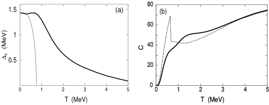
Figure 1: Neutron pairing gap (a) and heat capacity (b) for ¹²⁰Sn as functions of $T$. Solid and dotted lines show the MBCS and BCS gaps, respectively.

Shown in Fig. 1 (a) is the temperature dependence of the neutron pairing gap $\bar{\Delta}_{\nu}$ for ¹²⁰Sn, which is obtained from the MBCS equation (69) using the single-particle energies determined within the Woods-Saxon potential at $T=$ 0. The pairing parameter $G_{\nu}$ is chosen to be equal to 0.13 MeV, which yields $\bar{\Delta}(T=0)\equiv\bar{\Delta}(0)\simeq$ 1.4 MeV. Contrary to the BCS gap (dotted line), which collapses at $T_{\rm c}\simeq$ 0.79 MeV, the gap $\bar{\Delta}$ (solid line) does not vanish, but decreases monotonously with increasing $T$ at $T\geq$ 1 MeV resulting in a long tail up to $T\simeq$ 5 MeV. This behavior is caused by the thermal fluctuation of quasiparticle number in the MBCS equations (69). As the result, the heat capacity [Fig. 1 (b)] has no divergence at $T_{c}$, which is seen within the BCS theory.

4.2 Temperature dependence of GDR width

The GDR widths as a function of $T$ for ¹²⁰Sn obtained within the PDM are compared in Fig. 2 (a) with the experimental data and the prediction by the thermal fluctuation model (TFM) [16].

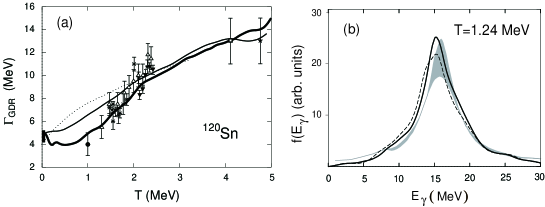
Figure 2: (b): GDR width $\Gamma_{\rm GDR}$ as a function of $T$ for ¹²⁰Sn. The thin and thick solid lines show the PDM results obtained neglecting pairing and including the renormalized gap $\widetilde{\Delta}=[1+1/\delta N^{2}]\bar{\Delta}$, respectively. The gap $\widetilde{\Delta}$ includes the correction $\delta N^{2}=\bar{\Delta}(0)^{2}\sum_{j}(j+1/2)/[(\epsilon_{j}-\bar{\epsilon}_{\rm F})^{2}+\bar{\Delta}(0)^{2}]$ due to an approximate number projection. The prediction by the TFM is shown as the dotted line ¹⁶; (b): GDR strength function at $T=$ 1.24 MeV. The dashed and solid lines show the results obtained without and including the gap $\widetilde{\Delta}$, while experimental results are shown as the shaded area.

The TFM interprets the broadening of the GDR width via an adiabatic coupling of GDR to quadrupole deformations induced by thermal fluctuations. Even when thermal pairing is neglected the PDM prediction, (the thin solid line) is already better than that given by the TFM, including the region of high $T$ where the width’s saturation is reported. The increase of the total width with $T$ is driven by the increase of the thermal width $\Gamma_{\rm T}$, which is caused by coupling to $pp$ and $hh$ configurations, since the quantal width $\Gamma_{\rm Q}$ is found to decrease slightly with increasing $T$ [12]. The inclusion of thermal pairing, which yields a sharper Fermi surface, compensates the smoothing of the Fermi surface with increasing $T$. This leads to a much weaker $T$-dependence of the GDR width at low $T$. As a result, the values of the width predicted by the PDM in this region significantly drop (the thick solid line), recovering the data point at $T=$ 1 MeV. The GDR strength function obtained including the MBCS gap is also closer to the experimental data than that obtained neglecting the thermal gap [Fig. 2 (b)].

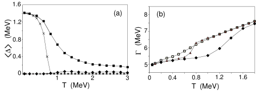
Figure 3: (a): Pairing gaps for ¹²⁰Sn averaged over thermal shape fluctuations versus $T$. Lines with triangles and crosses are the usual BCS proton and neutron pairing gaps, respectively, while those with diamonds and squares denote the corresponding pairing gaps, which also include thermal fluctuations of pairing fields. (b): GDR widths for ¹²⁰Sn versus $T$. Open squares, triangles, and diamonds denote the widths obtained without pairing, including BCS pairing, and thermally fluctuating pairing field from (a), respectively.

The results discussed above have also been confirmed by our recent calculations within a macroscopic approach, which takes pairing fluctuations into account along with the thermal shape fluctuations [17]. Here the free energies are calculated using the Nilsson-Strutinsky method at $T\neq$ 0, including thermal pairing correlations. The GDR is coupled to the nuclear shapes through a simple anisotropic harmonic oscillator model with a separable dipole-dipole interaction. The observables are averaged over the shape parameters and pairing gap. Our study reveals that the observed quenching of GDR width at low $T$ in ¹²⁰Sn and ¹⁴⁸Au can be understood in terms of simple shape effects caused by pairing correlations. Fluctuations in pairing field lead to a slowly vanishing pairing gap [Fig. 3 (a)], which influences the structural properties even at moderate $T$ ($\sim$1 MeV). We found that the low-$T$ structure and hence the GDR width are quite sensitive to the change of the pairing field [Fig. 3 (b)].

5 Conclusions

It has been shown in the present lecture that the MHFB and MBCS theories are microscopic approaches, which take into account thermal fluctuations of quasiparticle number. These large thermal fluctuations smooth out the sharp SN phase transition in finite nuclei. As a result, the thermal pairing gap does not collapse, but decreases monotonously with increasing temperature $T$, remaining finite even at $T$ as high as 4 - 5 MeV. This non-vanishing thermal pairing gap keeps the width of GDR remain almost constant at low $T$ ($\leq$ 1 MeV for ¹²⁰Sn) when it is included in the PDM. In this way the PDM becomes a semi-microscopic model that is able to describe the temperature dependence of the GDR width in a consistent way within a large temperature interval starting from very low $T$, where the GDR width is nearly $T$-independent, to the region when the width increases with $T$ (1 $\leq T\leq$ 3 - 4 MeV), and up to the region of high $T$ ($T>$ 4 - 5 MeV), where the width seems to saturate in tin isotopes.

References

• [1] L.D. Landau and E.M. Lifshitz, Course of Theoretical Physics, Vol. 5: Statistical Physics (Moscow, Nauka, 1964) pp. 297, 308.
• [2] M. Sano and S. Yamazaki, Prog. Theor. Phys. 29, 397 (1963).
• [3] A.L. Goodman, Nucl. Phys. A 352, 30 (1981).
• [4] A.L. Goodman, Phys. Rev. C 29, 1887 (1984).
• [5] L.G. Moretto, Phys. Lett. B 40, 1 (1972).
• [6] N. Dinh Dang, Z. Phys. A 335, 253 (1990).
• [7] N.D. Dang, P. Ring, and R. Rossignoli, Phys. Rev. C 47, 606 (1993).
• [8] N. Dinh Dang and V. Zelevinsky, Phys. Rev. C 64, 064319 (2001).
• [9] N. Dinh Dang and A. Arima, Phys. Rev. C 67, 014304 (2003).
• [10] N. Dinh Dang and A. Arima, Phys. Rev. C 68, 014318 (2003).
• [11] M.N. Harakeh and A. van der Woude, Giant resonances - Fundamental high-frequency modes of nuclear excitation (Oxford, Clarendon Press, 2001) p. 638.
• [12] N. Dinh Dang and A. Arima, Phys. Rev. Lett. 80, 4145 (1998); Nucl. Phys. A 636, 427 (1998).
• [13] N. Dinh Dang N. et al., Phys. Rev. C 63, 044302 (2001).
• [14] N.N. Bogolyubov and S. Tyablikov, Sov. Phys. Doklady 4, 6 (1959); D.N. Zubarev, Nonequilibrium Statistical Thermodynamics (Plenum, NY, 1974);
• [15] P.F. Bortignon P.F. et al., Nuc. Phys. A 460, 149 (1986); N. Dinh Dang, Nucl. Phys. A 504, 143 (1989).
• [16] D. Kuznesov et al., Phys. Rev. Lett. 81, 542 (1998).
• [17] P. Arumugam and N. Dinh Dang, RIKEN Accel. Prog. Rep. 39, 28 (2006).