Efficient matrix-vector products for large-scale nuclear Shell-Model calculations

Abstract

A method to accelerate the matrix-vector products of j-scheme nuclear Shell-Model Configuration Interaction (SMCI) calculations is presented. The method takes advantage of the matrix product form of the j-scheme proton-neutron Hamiltonian matrix. It is shown that the method can speed up unrestricted large-scale pf-shell calculations by up to two orders of magnitude compared to previously existing related j-scheme method. The new method allows unrestricted SMCI calculations up to j-scheme dimension $10^{10}$ to be made in more complex model spaces.

Introduction: The nuclear Shell-Model is the most general microscopic nuclear model and is in principle able to describe all properties of nuclei. Nuclear Shell-Model Configuration Interaction (SMCI) calculations in large and realistic single-particle (s.p.) model spaces are, however, very difficult to make due to the extremely large Hilbert space dimensions involved. The continuous increase in computing power has made it possible to make progressively larger nuclear SMCI calculations in restricted model spaces. Currently existing nuclear SMCI methods/programs make it possible to calculate nuclear wavefunctions exactly in the model spaces $sd$ and $pf$ Caurier et al. (1999) and in $pf_{5/2}g_{9/2}$ model space with somewhat truncated calculations. In larger model spaces drastic truncations (i.e. selection of allowed particle configurations) have to be made. Two basic problems arise in large-scale SMCI calculations: Large dimensions require huge amounts of storage space for the calculated states, and the number of non-zero Hamiltonian matrix elements becomes prohibitively large ($10^{14}-10^{16}$) even though the Hamiltonian matrix stays very sparse. Therefore both available memory and computational speed often become inadequate for the task at hand.

Using very large computing resources to solve SMCI problems is the brute force approach to circumvent these problems. Alternatives to it are to develop mathematical methods to truncate large calculations and to keep only physically relevant degrees of freedom in the wavefunctions, or to make the most time consuming parts of SMCI calculations more efficiently. Various truncation methods have been developed during the last twenty years, for example the methods that produce exponential convergence of observables as a function of truncation Horoi et al. (1994); Papenbrock et al. (2004); Andreozzi and Porrino (2001). A very good example of the methods that make SMCI calculations more efficient in terms of computation resource usage is being used in the SMCI code nathan and its cousin, the code antoine Nowacki and Caurier (1995); Caurier et al. (1999). These codes use a novel Hamiltonian matrix compression method where the SMCI proton-neutron Hamiltonian matrix elements are not stored before a SMCI calculation, but constructed during each matrix-vector operation of a Lanczos procedure using precalculated Reduced Density Matrix (RDM) elements. This innovation made it possible to make the first unrestricted SMCI calculations in the pf-shell Caurier et al. (1999), where other SMCI programs using older methods could not work without truncations. For example in the nucleus ${}^{56}{\rm Ni}$ in the pf-shell this method avoids the explicit storage of $10^{14}$ non-zero Hamiltonian matrix elements.

The most basic SMCI method is the m-scheme method Whitehead et al. (1977) that uses bare Slater determinants of spherically symmetric s.p. orbit configurations as its many-body basis states. The basic problem with the m-scheme SMCI is that the Slater determinant basis dimension is maximal and therefore a lot of storage (from gigabytes to tens of gigabytes) is needed for each calculated Lanczos basis vector in large-scale calculations. A common method to reduce the large matrix dimensions of the m-scheme SMCI is to use the existing symmetries of the nuclear Hamiltonian. The j-scheme SMCI method uses angular momentum projected many-body basis states, but does not have good isospin, and is used in the SMCI code nathan. Compared to the m-scheme the j-scheme typically reduces the SMCI dimensions by two orders of magnitude for low-spin states and less for high-spin states. This property makes it most suitable for low-spin states, such as the ground states of double-even nuclei. The j-scheme method Caurier et al. (1999); Nowacki and Caurier (1995) of matrix-vector products is further developed here to make it numerically more efficient and more suitable for very large SMCI calculations.

Theoretical overview: The j-scheme method forms the SMCI many-body basis states using angular momentum coupled products of proton and neutron many-body basis states. Lanczos vectors $|\vec{v}_{JM}\rangle$ are expanded as

$$|\vec{v}_{JM}\rangle = \sum_{j^{\prime}_{p}\alpha^{\prime}_{p}}\sum_{j^{\prime}_{n}\alpha^{\prime}_{n}}v^{j^{\prime}_{n}j^{\prime}_{p}J}_{\alpha^{\prime}_{n},\alpha^{\prime}_{p}}\left[|j^{\prime}_{n}\alpha^{\prime}_{n}\rangle|j^{\prime}_{p}\alpha^{\prime}_{p}\rangle\right]_{JM}\,.$$ (1)

where $j_{p}$ and $j_{n}$ are proton and neutron total angular momenta and the quantum numbers $\alpha_{p}$ and $\alpha_{n}$ sum over all possible combinations of linearly independent states. Because of the angular momentum coupled structure of basis states, the full Hamiltonian matrix can be naturally divided into matrix blocks that contain all allowed bra and ket particle configurations but where the proton and neutron bra and ket angular momenta are kept fixed. One such Hamiltonian matrix block will be concentrated on here. In addition, only the proton-neutron part of the nuclear two-body Hamiltonian is considered, whose treatment in the proton-neutron formalism is the most time consuming part of a j-scheme SMCI calculation.

Using the angular momentum coupled states of (1), the matrix elements of the nuclear proton-neutron Hamiltonian are sums of the products of proton one-body RDM elements, neutron RDM elements, angular momentum recoupling factors and transformed two-body interaction matrix elements:

$$H_{i+j,i^{\prime}+j^{\prime}} = \langle j_{n}\alpha_{n}j_{p}\alpha_{p};J|\hat{H}^{(2)}_{\rm pn}|j^{\prime}_{n}\alpha^{\prime}_{n}j^{\prime}_{p}\alpha^{\prime}_{p};J\rangle$$

$$= \sum_{aa^{\prime}bb^{\prime}\lambda}\Gamma^{\lambda}(j_{p}[\alpha_{p}]_{j}||[c^{\dagger}_{a}\tilde{c}_{{a^{\prime}}}]_{\lambda}||j_{p}^{\prime}[\alpha_{p}^{\prime}]_{j^{\prime}})(j_{n}[\alpha_{n}]_{i}||[c^{\dagger}_{b}\tilde{c}_{{b^{\prime}}}]_{\lambda}||j_{n}^{\prime}[\alpha_{n}^{\prime}]_{i^{\prime}})F_{\lambda}(aa^{\prime}bb^{\prime})\,,$$

as originally shown by French French et al. (1969). $F_{\lambda}(aa^{\prime}bb^{\prime})$ are particle-hole transformed two-body interaction matrix elements and $\Gamma^{\lambda}$ is an angular momentum recoupling factor (see Caurier et al. (2005) for more details). Eq. (2) shows the principal idea of Caurier et al. (1999); Nowacki and Caurier (1995): Create row and column indices for proton and neutron RDM elements in such a way that the indices of the full Hamiltonian matrix can be obtained just by summing together the proton and neutron indices. In this way a small amount of RDM elements can generate a large number of Hamiltonian matrix elements. The method of Eq. (2) will now be extended. To simplify the subsequent formulae the $d_{1}\times d_{1}^{\prime}$ neutron RDM is written as

$$(j_{n}[\alpha_{n}]_{j}||[c^{\dagger}_{a}\tilde{c}_{{a^{\prime}}}]_{\lambda}||j_{n}^{\prime}[\alpha_{n}^{\prime}]_{j^{\prime}})\equiv A^{aa^{\prime}\lambda}_{jj^{\prime}}\,,$$ (2)

where $j\in[1,d_{1}]$ and $j^{\prime}\in[1,d^{\prime}_{1}]$ and the $d_{2}\times d_{2}^{\prime}$ proton RDM as

$$(j_{p}[\alpha_{p}]_{i}||[c^{\dagger}_{b}\tilde{c}_{{b^{\prime}}}]_{\lambda}||j_{p}^{\prime}[\alpha_{p}^{\prime}]_{i^{\prime}})\equiv B^{bb^{\prime}\lambda}_{ii^{\prime}}\,,$$ (3)

where $i\in[1,d_{2}]$ and $i^{\prime}\in[1,d^{\prime}_{2}]$. Inside the RDMs ${\bf A}$ and ${\bf B}$ each set of quantum numbers $[\alpha_{n}]$ has a unique row or column index $i$. The density operator indices label sets of s.p. quantum numbers, $a=\left\{n_{a},l_{a},j_{a}\right\}$, $b=\left\{n_{b},l_{b},j_{b}\right\}$. Since each density operator only connects one bra particle configuration to one ket configuration, the matrices ${\bf A}$ and ${\bf B}$ are sparse supermatrices that consist of dense blocks. Furthermore, a matrix ${\bf A}^{aa^{\prime}\lambda}$ that corresponds to a certain density operator $\bigl{[}c^{\dagger}_{a}\tilde{c}_{a^{\prime}}\bigr{]}_{\lambda}$ has only one dense matrix block on each supermatrix block row.

A Lanczos basis vector $|{\vec{v}}_{JM}\rangle$ and the result of a Hamiltonian matrix-vector product $|{\vec{u}}_{JM}\rangle={\hat{H}}|{\vec{v}}_{JM}\rangle$ can be ordered so that their basis state amplitudes can be expressed in terms of matrices:

$$|\vec{v}_{JM}\rangle = \sum_{j^{\prime}=1}^{d^{\prime}_{2}}\sum_{i^{\prime}=1}^{d^{\prime}_{1}}v^{j^{\prime}_{n}j^{\prime}_{p}J}_{d_{1}(j^{\prime}-1)+i^{\prime}}\left[|j^{\prime}_{n}[\alpha^{\prime}_{n}]_{i^{\prime}}\rangle|j^{\prime}_{p}[\alpha^{\prime}_{p}]_{j^{\prime}}\rangle\right]_{JM}\,,$$ (4)

$$\equiv \sum_{j^{\prime}=1}^{d^{\prime}_{2}}\sum_{i^{\prime}=1}^{d^{\prime}_{1}}V_{i^{\prime}j^{\prime}}\left[|j^{\prime}_{n}[\alpha^{\prime}_{n}]_{i^{\prime}}\rangle|j^{\prime}_{p}[\alpha^{\prime}_{p}]_{j^{\prime}}\rangle\right]_{JM}\,,$$

and similarly for the vector $|\vec{u}_{JM}\rangle$ where the constant quantum numbers have been omitted for simplicity. Using Eqs. (2-5), the Hamiltonian matrix of Eq. (2) can be transformed to sums over direct products of proton and neutron density matrices and the matrix-vector product can be expressed as a sum of triple matrix products:

$$U_{ji} \equiv u_{(i-1)d_{1}+j}=H_{(i-1)d_{1}+j,(i^{\prime}-1)d^{\prime}_{1}+j^{\prime}}v_{(i^{\prime}-1)d^{\prime}_{1}+j^{\prime}}$$ (5)

$$= \sum_{\lambda aa^{\prime}bb^{\prime}}\Gamma^{\lambda}F_{\lambda}(aa^{\prime}bb^{\prime})A^{aa^{\prime}\lambda}_{jj^{\prime}}B^{bb^{\prime}\lambda}_{ii^{\prime}}v_{(i^{\prime}-1)d^{\prime}_{1}+j^{\prime}}$$

$$= \sum_{\lambda bb^{\prime}}\Bigl{(}\sum_{aa^{\prime}}\Gamma^{\lambda}F_{\lambda}(aa^{\prime}bb^{\prime})A^{aa^{\prime}\lambda}_{jj^{\prime}}\Bigr{)}V_{j^{\prime}i^{\prime}}B^{bb^{\prime}\lambda}_{ii^{\prime}}\,.$$

In this equation the indices $i^{\prime}$ and $j^{\prime}$ are implicitly summed over. Alternatively, one may change the order of the matrix products and use the equation

$$U_{ji}=\sum_{\lambda aa^{\prime}}A^{aa^{\prime}\lambda}_{jj^{\prime}}V_{j^{\prime}i^{\prime}}\Bigl{(}\sum_{bb^{\prime}}\Gamma^{\lambda}F_{\lambda}(aa^{\prime}bb^{\prime})B^{bb^{\prime}\lambda}_{ii^{\prime}}\Bigr{)}\,,$$ (6)

if it uses less sum and multiplication operations. Usually for $N_{v}\neq Z_{v}$ nuclei the density matrices corresponding to smaller number of valence particles/holes are smaller and should be used in the innermost loop. Eqs. (6) and (7) can still be further optimised. Because the same density matrix ${\bf A}^{aa^{\prime}\lambda}$ is used for more than one Hamiltonian block, Eq. (6) can be converted to the form

$$U_{ji}=\sum_{\lambda bb^{\prime}}\Bigl{(}\sum_{aa^{\prime}}F_{\lambda}(aa^{\prime}bb^{\prime})A^{aa^{\prime}\lambda}_{jj^{\prime}}\Bigr{)}\sum_{j^{\prime}_{n}}\Gamma^{\lambda}V^{j^{\prime}_{n}}_{j^{\prime}i^{\prime}}B^{bb^{\prime}\lambda j^{\prime}_{n}}_{ii^{\prime}}$$ (7)

where the quantum number $j^{\prime}_{n}$ of a neutron many-body basis state goes through all neutron angular momenta quantum numbers that can be coupled with fixed proton ket angular momentum quantum number $j^{\prime}_{p}$ to a total angular momentum $J$. In this way multiple right-hand side matrices ${\bf V}^{j^{\prime}_{n}}$ can be multiplied with their corresponding density matrices ${\bf B}^{bb^{\prime}\lambda j^{\prime}_{n}}$ and summed together before performing the multiplications with the blocks of matrix ${\bf A}^{aa^{\prime}\lambda}$. Eq. (8) reduces to Eq. (6) for $J=0$ states, but reduces floating point operations for states with higher angular momentum by approximately $30-50$%. It is however quite complex to implement and therefore has not yet been used in this work. Note: The form of Eqs. (6-7) makes them ideal for separable interactions, such as the pairing plus quadrupole interaction ${\hat{H}}^{(2)}=-G{\hat{P}}^{\dagger}{\hat{P}}-{\textstyle{1\over 2}}\chi\sum_{\mu}{\hat{Q}}^{\dagger}_{\mu}{\hat{Q}}_{\mu}$ or the center-of-mass interaction Lawson (1979), because the resulting separability of the two-body interaction matrix elements, $F_{\lambda}(aa^{\prime}bb^{\prime})=f_{\lambda}(aa^{\prime})f_{\lambda}(bb^{\prime})$, allows the full matrices $\bf A$ and $\bf B$ in Eqs. (6-8) to be used totally independently of each other.

Discussion: The results of unrestricted benchmark calculations made in the pf-shell model space for nuclei from ${}^{44}{\rm Ti}$ to ${}^{56}{\rm Ni}$ using an implementation of this method in the SMCI code eicode Toivanen (2004); Kortelainen et al. (2006) are presented in Fig. 1. All results are calculated using one AMD Opteron $2.4$ GHz processor. It can be seen that the number of mathematical operations per one Hamiltonian matrix-vector product scales as $d^{1.46}$ for angular momenta $J=0,2$ where $d$ is the SMCI matrix dimension. The number of mathematical operations for higher angular momenta (which have exactly the same scaling) have not been included for clarity. In this work the best implementation of the original j-scheme matrix vector product method of Caurier et al. (1999); Nowacki and Caurier (1995) scales as $d^{1.82}$ as a function of basis dimension (Fig. 1, dashed line). Whereas calculations for all angular momentum values scale exactly similarly in the case of the old method, the new method has slightly different constant multiplicative factors that depend on angular momentum and the isospin z-component. The dependence on angular momentum is roughly $2J+1$ and can be removed to a large extent by using Eq. (8) for matrix-vector products instead of Eqs. (6-7). Both the old method and the method of Eqs. (6-7) use the largest number of floating point operations for nuclei with $N_{v}=Z_{v}$, and therefore the wavefunctions of these nuclei are the most time consuming ones to calculate.

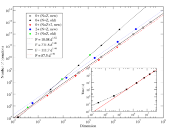
Figure 1: (Color online) Number of mathematical operations needed for one matrix-vector product as a function of basis dimension for various $N_{v}=Z_{v}$ and $N_{v}=Z_{v}+2$ pf-shell nuclei from ${}^{44}{\rm Ti}$ to ${}^{60}{\rm Zn}$. The lines are fit functions, shown in the legend box. Inset: Actual time per one matrix vector operation for $0^{+}$ states of $N_{v}=Z_{v}$ pf-shell nuclei using the new method. The solid line is a fitted function $F=8.28\cdot 10^{-7}d^{1.28}$.

The more favourable scaling of floating point operations in this modified method reduces them significantly for very large calculations. In the case of $0^{+}$ states of ${}^{56}{\rm Ni}$ the reduction of floating point operations is $35$-fold. Considering the actual matrix-vector product times, the time plot in Fig. 1 inset shows two different regimes. In the low-dimensional cases matrix products are very fast, initialisation overheads dominate the calculation time, and therefore only the scaling of matrix-vector operation times in the higher-dimensional regime from ${}^{50}{\rm Mn}$ onwards are of interest. In this regime the matrix-vector operation times scale as $n^{1.28}$. This scaling can be compared against the $n^{1.1}$ scaling of the m-scheme code antoine, shown on page 445 of Caurier et al. (2005) where the time for $15$ Lanczos iterations for $0^{+}$ states of the pf-shell nucleus ${}^{52}{\rm Fe}$ is roughly $10^{4}$ seconds and roughly $10^{5}$ seconds for ${}^{56}{\rm Ni}$ (extrapolated), giving average matrix-vector multiplication times of $670$ and $6700$ seconds using a modern microprocessor comparable to the one used in this work. For the same two calculations the new j-scheme method that uses Eqs. (6) and (7) results with one Hamiltonian matrix-vector multiplication taking respectively $83$ and $1317$s. The code antoine is therefore five times slower than the new j-scheme method of Eqs. (6-7) for ${}^{56}{\rm Ni}$. Compared to the original j-scheme method of  Caurier et al. (1999); Nowacki and Caurier (1995), used in eicode, the new method shortens the calculation time $75$-fold for this nucleus.

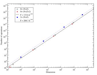
Figure 2: (Color online) Same as Fig. 1, but for unrestricted calculations for $N=Z$ and $N=Z+2$ nuclei in the $sdg_{7/2}h_{11/2}$ model space using the method of Eqs. (6-7).

The reason why the new method is faster than what the reduction of the number of mathematical operations alone in Fig. 1 suggests, is that the matrix products of Eqs. (6-7) can be implemented very efficiently on a modern computer using fast matrix product kernel routines Goto and van de Geijn (2005). For large SMCI calculations, where the RDM blocks have large dimensions, the new method can use up to $70\%$ of a processor’s theoretical peak floating point capacity in the pf-shell model space and even slightly more in larger s.p. model spaces. In contrast, the efficiency of the best implementation of the original j-scheme method of Caurier et al. (1999) in the code eicode is always low, roughly $10-15\%$ of the processor’s peak capacity. Looking at the calculation time plot of Caurier et al. (2005) it is suspected that this is also the case for the codes antoine and nathan. The reasons for this inefficiency are the explicit calculation of matrix indices and the explicit construction of every Hamiltonian matrix element, which are avoided in the new method.

Conclusions: It has been shown that the numerical effort needed to use the optimised j-scheme matrix-vector products of Eqs. (6-7) scales more favourably than the old j-scheme method, used in the SMCI codes nathan and eicode, as a function of basis dimension, making the new method up to two orders of magnitude faster in the pf-shell. The same speedup and scaling of floating point operations also happens in the ${\rm sd}{\rm g}_{7/2}{\rm h}_{11/2}$ model space used for nuclei above ${}^{100}{\rm Sn}$. This can be seen from Fig. 2, where the scaling of floating point operations has been plotted for various $N_{v},Z_{v}=3-8$ nuclei in this model space. The increased efficiency makes the method competitive against the m-scheme SMCI method of Caurier et al. (1999); Nowacki and Caurier (1995) that is used in most modern m-scheme SMCI codes.

Table 1: M-scheme and j-scheme dimensions, number of floating point operations and estimated computation time with one CPU for various unrestricted SMCI calculations for the $0^{+}$ states of nuclei in the $sdg_{7/2}h_{11/2}$ model space. $N_{v}$ and $Z_{v}$ are the number of valence neutrons and protons.

$(N_{v},Z_{v})$	Dim (m)	Dim (j)	$F$	$T_{1}$[s]
$(6,4)$	$8.56\cdot 10^{8}$	$7.24\cdot 10^{6}$	$1.38\cdot 10^{12}$	$550$
$(5,5)$	$1.06\cdot 10^{9}$	$8.92\cdot 10^{6}$	$1.73\cdot 10^{12}$	$870$
$(7,5)$	$1.65\cdot 10^{10}$	$1.21\cdot 10^{8}$	$8.45\cdot 10^{13}$	$2.9\cdot 10^{4}$
$(6,6)$	$2.00\cdot 10^{10}$	$1.45\cdot 10^{8}$	$1.02\cdot 10^{14}$	$3.4\cdot 10^{4}$
$(8,6)$	$2.20\cdot 10^{11}$	$1.43\cdot 10^{9}$	$3.11\cdot 10^{15}$	$1.03\cdot 10^{6}$
$(8,8)$	$2.43\cdot 10^{12}$	$1.50\cdot 10^{9}$	$3.08\cdot 10^{15}$	$1.02\cdot 10^{6}$

With the j-scheme matrix vector product method shown here it is possible to make unrestricted SMCI calculations for all nuclei in the ${\rm pf}$ model space and for most nuclei in the ${\rm pf}_{5/2}{\rm g}_{9/2}$ model space using modest computing resources. For more complex model spaces more computational power will be necessary, but calculations still stay tractable, since j-scheme dimensions of the order of $2\cdot 10^{9}$ can be handled easily. Table 1 shows estimated matrix-vector product times for various nuclei in the $sdg_{7/2}h_{11/2}$ model space for up to eight valence protons and neutron holes. For up to $10$ valence particles+holes the method of Eqs. (6-7) can be used without large computational resources. The calculations with more than $10$ valence particles need larger computational resources. Using the original j-scheme method of Caurier et al. (1999); Nowacki and Caurier (1995), at least two orders of magnitude more resources would have to be used to obtain results equally quickly for large-scale calculations. The m-scheme SMCI methods also encounter their dimensionality problem with these nuclei.

Dimensions of the same order of magnitude as in Table 1 will also be encountered in the $pf_{5/2}g_{7/2}d_{5/2}$ model space that is used for the description of deformed nuclei in the $N\approx Z=40$ region and with the No-Core Shell-Model (NCSM) Navrátil et al. (2006) used for the ab initio description of the structure of light nuclei. The method described here makes it possible to do j-scheme SMCI calculations up to a dimension of $10^{10}$ with current computing hardware and is a step towards unrestricted calculations in the aforementioned model spaces. A further increase of SMCI calculation dimensions can be sought for by combining this method with the advanced truncation methods that show exponential convergence, such as the methods of Refs. Horoi et al. (1994); Andreozzi and Porrino (2001); Papenbrock et al. (2004).

References

- Caurier et al. (1999) E. Caurier, G. Martinez-Pinedo, F. Nowacki, A. Poves, J. Retamosa, and A. P. Zuker, Phys. Rev. C 59, 2033 (1999).
- Horoi et al. (1994) M. Horoi, B. A. Brown, and V. Zelevinsky, Phys. Rev. C 50 (1994).
- Papenbrock et al. (2004) T. Papenbrock, A. Juogadalvis, and D. J. Dean, Phys. Rev. C 69, 024312 (2004).
- Andreozzi and Porrino (2001) F. Andreozzi and A. Porrino, J. Phys. G 27, 845 (2001).
- Nowacki and Caurier (1995) F. Nowacki and E. Caurier, CRN, Strasbourg (1995).
- Whitehead et al. (1977) R. R. Whitehead, A. Watt, B. J. Cole, and I. Morrison, Adv. Nucl. Phys. 9, 123 (1977).
- French et al. (1969) J. B. French, C. E. Halbert, J. B. McGrory, and S. S. M. Wong, Adv. Nucl. Phys. 3, 237 (1969).
- Caurier et al. (2005) E. Caurier, G. Martinez-Pinedo, F. Novacki, A. Poves, and A. P. Zuker, Rev. Mod. Phys. 77, 427 (2005).
- Lawson (1979) R. D. Lawson, ”Theory of the Nuclear Shell Model”, Oxford (1979).
- Toivanen (2004) J. Toivanen, computer code EICODE, JYFL, Finland (2004).
- Kortelainen et al. (2006) M. Kortelainen, T. Kosmas, J. Suhonen, and J. Toivanen, Phys. Lett. B 632, 226 (2006).
- Goto and van de Geijn (2005) K. Goto and R. van de Geijn, ACM Transactions on Mathematical Software, under revision (2005).
- Navrátil et al. (2006) P. Navrátil, C. A. Bertulani, and E. Caurier, Phys. Rev. C 73, 065801 (2006).