Isospin symmetry in mirror $\alpha$-decays

Abstract

We show that a consequence of isospin symmetry, recently discovered in mirror conjugated one-nucleon decays, can be extended to mirror-conjugated $\alpha$-particles decays, both virtual and real. For virtual $\alpha$-decays of bound mirror pairs this symmetry manifests itself as a relation between the Asymptotic Normalization Coefficients (ANCs) of $\alpha$-particle overlap integrals. This relation is given by a simple analytical formula which involves $\alpha$-particle separation energies and charges of residual nuclei. For bound-unbound mirror pairs, the ANC of a bound nucleus is related to the $\alpha$-width of the mirror unbound level. For unbound mirror pairs we get a new analytical formula that relates the widths of mirror resonances. We test the validity of these analytical formuli against the predictions of a two-body potential and of a many-body microscopic cluster model for several mirror states in ⁷Li-⁷Be, ¹¹B-¹¹C and ¹⁹F-¹⁹Ne isotopes. We show that these analytical formulae are valid in many cases but that some deviations can be expected for isotopes with strongly deformed and easily excited cores. In general, the results from microscopic model are not very sensitive to model assumptions and can be used to predict unknown astrophysically relevant cross sections using known information about mirror systems.

I Introduction

In the last few years, it has been realised that charge symmetry of nucleon-nucleon (NN) interaction leads to specific relations between the amplitudes of mirror-conjugated one-nucleon decays ${}^{A}_{N}Z\rightarrow^{A-1}_{N-1}Z+n$ and ${}^{A}_{Z}N\rightarrow^{A-1}_{Z-1}N+p$ Tim03 . In a mirror pair of bound states this symmetry links Asymptotic Normalization Coefficients (ANCs) for mirror-conjugated overlap integrals $\langle^{A}_{N}Z|^{A-1}_{N-1}Z\otimes n\rangle$ and $\langle^{A}_{Z}N|^{A-1}_{Z-1}N\otimes p\rangle$. In bound-unbound mirror states, it manifests itself as a link between the neutron ANC and the width of the mirror proton resonance. In both cases this link can be represented by an approximate simple model-independent analytical formula that contains only nucleon binding energies, nuclear charges and the range of the strong nucleon-core interaction Tim03 . Comparison with microscopic cluster model calculations Tim05a ; Tim05b has shown that the average accuracy of this formula is about 7$\%$ for bound mirror pairs Tim05a and 10$\%$ for bound-unbound mirror pairs Tim05b .

The knowledge of the link between mirror ANCs can be beneficial for predicting unknown ANCs using the unformation about known mirror ANCs. The latter can be used in nuclear astrophysics to predict or verify nucleon capture cross sections at stellar energies. Thus, the proton ANCs for ⁸B, ⁹C, ¹²N and ²⁷P have been determined using the measured neutron ANCs for their mirror analogs ⁸Li Tra03 , ⁹Li Guo05 , ¹²B TI and ²⁷Mg Guo06 respectively, and then have been used to predict the astrophysical $S$-factors for the corresponding non-resonant (p,$\gamma$) reactions on ⁷Be, ⁸B, ¹¹C and ²⁶Si at low energies. Also, the isospin symmetry in bound-unbound mirror pairs has been used to predict the neutron ANC for the halo nucleus ¹⁵C($\frac{1}{2}^{+}$) and the low-energy cross section for the ¹⁴C(n,$\gamma)^{15}$C($\frac{1}{2}^{+}$) reaction using the measured width of the proton resonance ¹⁵F($\frac{1}{2}^{+}$) Tim06a .

In this paper, we show that similar consequences of isospin symmetry are present in mirror-conjugated $\alpha$-decays. Their knowledge may be used in nuclear astrophysics to predict important ($\alpha,\gamma$), ($\alpha$,N) and (N,$\alpha$) cross sections.

In Sec.II.A we consider bound mirror pairs and derive a simple analytical formula for the ratio of mirror ANCs squared. As in the case of nucleon decays, the formula depends only on mirror $\alpha$-particle binding energies, nuclear charges and the range of the $\alpha$-core potential. We test this formula for the two-body model, where exact numerical solutions are available. In Sec. II.B we make predictions in the microscopic cluster model (MCM) for the ANCs of bound mirror pairs ⁷Li-⁷Be, ¹¹B-¹¹C and ¹⁹F-¹⁹Ne in which the $\alpha$-decay threshold in the lowest. All three mirror pairs are important for nuclear astrophysics applications. In Sec. III we consider bound-unbound mirror states of the same pairs of nuclei both in a two-body model and in the MCM. In Sec. IV we discuss isospin symmetry in mirror resonance states and in Sec. V we summarise the results obtained and draw conclusions.

II Bound mirror pairs

II.1 Two-body model with charge-independent $\alpha$-core strong interaction

We consider (1) a bound system ${}^{A-4}_{Z-2}(N-2)+\alpha$ and (2) its bound mirror analog ${}^{A-4}_{N-2}(Z-2)+\alpha$ in a two-body model. We order these systems is such a way that the binding energy $\varepsilon_{1}$ of the first system is larger than the second binding energy $\varepsilon_{2}$. We denote this two cores as $X_{1}$ and $X_{2}$ and assume that the nuclear $\alpha-X_{i}$ interaction $V_{N}$ in mirror systems is exactly the same so that all the difference in the wave functions $\Psi_{1}$ and $\Psi_{2}$ of these mirror systems is determined by different Coulomb interactions $V_{C_{1}}$ and $V_{C_{2}}$. In practice, the two mirror $\alpha$-particle wave functions are close to each other both in the internal nuclear region and on the surface, where the $\alpha-X_{i}$ potential strongly decreases.

The wave function $\Psi_{i}$, where $i$ = 1,2, satisfies the Schrödinger equation

$$(T+V_{N}+V_{C_{i}}+\varepsilon_{i})\Psi_{i}=0$$ (1)

with binding energy $\varepsilon_{i}$. The radial part $\Psi^{(i)}_{l}(r)$ corresponds to the orbital momentum $l$ behaves asymptotically as

$$\Psi^{(i)}_{l}(r)\approx C^{(i)}_{l}W_{-\eta_{i},l+1/2}(2\kappa_{i}r)/r.$$ (2)

Here $C^{(i)}_{l}$ is the $\alpha$-particle ANC, $W$ is the Whittaker function, $\kappa_{i}=\sqrt{2\mu\varepsilon_{i}}/\hbar$, $\mu$ is the reduced mass for the $\alpha+X_{i}$ system (we neglect the $i$ dependence of $\mu$) and $\eta_{i}=Z_{i}Z_{\alpha}e^{2}\mu/\hbar^{2}\kappa_{i}$.

The ANC $C^{(i)}_{l}$ can be represented by the integral

$$C^{(i)}_{l}=-\frac{2\mu}{\hbar^{2}}\int_{0}^{\infty}dr\,r^{2}\tilde{\phi}_{l}^{(i)}(r)(V_{N}+V_{C_{i}}-\tilde{V}_{i})\Psi^{(i)}_{l}(r),$$ (3)

where the function $\tilde{\phi}_{l}^{(i)}$ is the regular solution of the Schrödinger equation with an arbitrary potential $\tilde{V}_{i}$

$$(T_{l}+\tilde{V}_{i}+\varepsilon_{i})\tilde{\phi}_{l}^{(i)}=0,$$ (4)

with the boundary condition

$$\tilde{\phi}_{l}^{(1)}(r)\rightarrow\phi_{l}^{(1)}(r)=e^{-\frac{\pi i}{2}(l+1+\eta_{1})}F_{l}(i\kappa_{1}r)/\kappa_{1}r,$$ (5)

for $r\rightarrow\infty$, where $F$ is the regular Coulomb function. The only requirement on the potential $\tilde{V}_{i}$ is that at large distances $r$ it should cancel the long-range Coulomb interaction potential $V_{C_{i}}$ between $\alpha$ and $X_{i}$ in order to provide convergence for the integral (3).

We exploit the freedom in choosing the $\tilde{V}_{1}$ to separate out from the formula (3) for $C^{(2)}_{l}$ a term which looks as close as possible to the corresponding formula for $C^{(1)}_{l}$. We choose $\tilde{V}_{1}$ to be the Coulomb interaction $V_{C_{0}}^{(1)}$ between a point $\alpha$-particle and a point core $X_{1}$ so that

$$\tilde{\phi}_{l}^{(1)}(r)=\phi_{l}^{(1)}(r)=e^{-\frac{\pi i}{2}(l+1+\eta_{1})}F_{l}(i\kappa_{1}r)/\kappa_{1}r$$ (6)

for all $r$. We next choose $\tilde{V}_{2}$ so that $\tilde{\phi}_{l}^{(2)}(r)$ is proportional to $\tilde{\phi}_{l}^{(1)}(r)$ for a range of values of $r<a$ that will be specified later. For $r>a$ the general requirement for the $\tilde{V}_{2}$ at large distances must be satisfied, so we define

$$\tilde{V}_{2}=\varepsilon_{1}-\varepsilon_{2}+V_{C_{0}}^{(1)}, r<a$$

$$\tilde{V}_{2}=V_{C_{0}}^{(2)}, r\geq a,$$ (7)

With this choice in Eq. (4) the function $\tilde{\phi}_{l}^{(2)}(r)$ is the regular solution of the Schrödinger equation

$$(T_{l}+V_{C_{0}}^{(1)}+\varepsilon_{1})\tilde{\phi}_{l}^{(2)}(r)=0, r<a$$

$$(T_{l}+V_{C_{0}}^{(2)}+\varepsilon_{2})\tilde{\phi}_{l}^{(2)}(r)=0, r\geq a.$$ (8)

and is therefore proportional to $\phi_{l}^{(1)}(r)$ for $r<a$. Its explicit form is

$$\tilde{\phi}_{l}^{(2)}(r)=A\phi_{l}^{(1)}(r), r\leq a$$

$$\tilde{\phi}_{l}^{(2)}(r)=\phi_{l}^{(2)}(r)+BW_{-\eta_{2},l+1/2}(2\kappa_{2}r)/r. r\geq a$$ (9)

The coefficients $A$ and $B$ are found from continuity of $\tilde{\phi}_{l}^{(2)}(r)$ and its derivative at $r=a$:

$$A=A_{0}(a)+BW_{2}/a\phi_{l}^{(1)}$$ (10)

where

$$A_{0}(a)=\phi_{l}^{(2)}(a)/\phi_{l}^{(1)}(a),$$ (11)

$$B=A^{\prime}_{0}(a)/(W_{2}/a\phi_{l}^{(1)})^{\prime}$$

(12)

Here the notation $W_{2}$ for $W_{-\eta_{2},l+1/2}(2\kappa_{2}r)$ is introduced and the ^′ denotes the differentiation with respect to $a$. With these choices for the $\tilde{V}_{i}$ the formula (3) becomes

$$-\frac{\hbar^{2}}{2\mu}C^{(2)}_{l}=A\int_{0}^{a}dr\,r^{2}\phi_{l}^{(1)}(V_{N}+\Delta V_{C_{1}})\Psi^{(2)}_{l}$$

$$+\int_{a}^{\infty}dr\,r^{2}\tilde{\phi}_{l}^{(2)}(V_{N}+\Delta V_{C_{2}})\Psi^{(2)}_{l}+R_{C}(a)$$ (13)

where

$$\Delta V_{C_{i}}=V_{C_{i}}-V^{(i)}_{C_{0}}$$ (14)

and

$$R_{C}(a)=A\int_{0}^{a}dr\,r^{2}\phi_{l}^{(1)}(V_{C_{2}}-V_{C_{1}}-\varepsilon_{1}+\varepsilon_{2})\Psi^{(2)}_{l}.$$

(15)

Introducing new functions

$$\Delta\Psi_{12}=\Psi^{(2)}_{l}-\Psi^{(1)}_{l}$$ (16)

and

$$\delta\phi_{12}(r,a)=\phi_{l}^{(2)}(r)-A_{0}(a)\phi_{l}^{(1)}(r),$$ (17)

and rearranging all terms in Eq. (13) is such a way that integrals from $a$ to $\infty$ do not contain products $\phi_{l}^{(1)}(r)\Psi^{(2)}_{l}(r)$ which increase with $r$, we get

$$-\frac{\hbar^{2}}{2\mu}C^{(2)}_{l}=A_{0}(a)\int_{0}^{\infty}dr\,r^{2}\phi_{l}^{(1)}(V_{N}+\Delta V_{C_{1})})\Psi^{(1)}_{l}$$

$$+R_{C}(a)+R_{\Delta\Psi}+R_{\delta\phi}(a)+R_{B}(a)+R_{\Delta V_{C}}(a),$$

(18)

where the first term of the r.h.s. of the Eq. (18 ) is nothing but $-\hbar^{2}/2\mu A_{0}(a)C^{(1)}_{l}$.

We will show that all the five remainder terms in Eq. (18) are small compared with either $-\hbar^{2}/2\mu A_{0}(a)C^{(1)}_{l}$ or $-\hbar^{2}/2\mu C^{(2)}_{l}$ provided the radius $a$ is chosen in a specific way.

The term $R_{C}(a)$ is negligible for $a<R_{N}$, where $R_{N}$ is the radius of the nuclear interior, because both the Coulomb diffefence $V_{C_{2}}-V_{C_{1}}$ and the binding energy difference $\varepsilon_{1}-\varepsilon_{2}$ are small compared with the nuclear potential $V_{N}$. For $a>R_{N}$, $R_{C}(a)$ grows because the function $\phi_{l}^{(1)}$ increases faster than $\Psi^{(2)}_{l}$ decreases.

The contribution from $R_{\Delta\Psi}$, where

$$R_{\Delta\Psi}=\int_{0}^{\infty}dr\,r^{2}\phi_{l}^{(2)}(V_{N}+\Delta V_{C_{1}})\Delta\Psi_{12},$$ (19)

does not depend on $a$ and is determined by the difference between the functions $\Psi^{(2)}_{l}$ and $\Psi^{(1)}_{l}$ in the region that gives the most contribution to the integral in the r.h.s. of Eq. (19). In the cases considered below, this difference is about 2$\%$.

The term $R_{\delta\phi}(a)$ defined as

$$R_{\delta\phi}(a)=\int_{a}^{\infty}dr\,r^{2}\delta\phi_{12}(r,a)V_{N}\Psi^{(1)}_{l}$$

$$-\int_{0}^{a}dr\,r^{2}\delta\phi_{12}(r,a)V_{N}\Delta\Psi_{12},$$ (20)

contains the function $\delta\phi_{12}(r,a)$ which is equal to zero at $r=a$. Therefore, if $a$ is at a point where $V_{N}\Psi^{(1)}_{l}$ reaches its maximum and is a decreasing function at $r>a$ then the contribution from $R_{\delta\phi}(a)$ will be small.This point can be chosen to be the nuclear radius $R_{N}$, which for $\alpha+X$ system is about (1.1-1.3)(4^1/3+$X^{1/3}$). If at the same time $\phi_{l}^{(2)}(r)/\phi_{l}^{(1)}(r)$ varies slowly with $r$ around $a$ then $\phi_{12}(r,a)\approx 0$ which guarantees that $R_{\delta\phi}(a)$ is negligible. However, $R_{\delta\phi}(a)$ increases if $a<R_{N}$ and $\phi_{l}^{(2)}/\phi_{l}^{(1)}$ at $r=R_{N}$ differs from $A_{0}(a)$. On the other hand, $R_{\delta\phi}(a)$ is very small for $a>R_{N}$.

The next term,

$$R_{B}(a)=B\int_{a}^{\infty}dr\,r\,W_{2}(V_{N}+\Delta V_{C_{2}})\Psi^{(2)}_{l}$$

$$+B\frac{W_{2}}{a\phi_{l}^{(1)}}\int_{0}^{a}dr\,r^{2}\phi_{l}^{(1)}(V_{N}+\Delta V_{C_{1}})\Psi^{(2)}_{l},$$ (21)

depends on $B$. The $B$ is zero at two points, at $a=0$ and at $a=a_{m}$ where the function $A_{0}(a)$ reaches its maximum (or in other words $A^{\prime}_{0}(a_{m})=0$). At all other points the contribution from $R_{B}(a)$ depends on how large is $BW_{2}/a\phi^{(1)}_{l}$ with respect to $A_{0}(a)$. We show in Appendix that

$$\frac{BW_{2}}{a\phi^{(1)}_{l}A_{0}(a)}=\frac{p_{2}(a)-p_{1}(a)}{p_{2}(a)+p_{1}(a)},$$ (22)

where

$$p_{i}(a)=\sqrt{\frac{2\eta_{i}\kappa_{i}}{r}+\frac{l(l+1)}{r^{2}}+\kappa_{i}^{2}}.$$ (23)

For mirror $\alpha$ states $p_{2}(a)$ does not differ much from $p_{1}(a)$, especially near $a\approx R_{N}$. Thus $BW_{2}/a\phi^{(1)}_{l}<<A_{0}(a)$ and, therefore, $R_{B}(R_{N})$ will be small compared with $-\hbar^{2}/2\mu A_{0}(a)C^{(1)}_{l}$.

The last term,

$$R_{\Delta V_{C}}(a)=\int_{a}^{\infty}dr\,r^{2}(\phi_{l}^{(2)}\Delta V_{C_{2}}-A_{0}(a)\phi_{l}^{(1)}\Delta V_{C_{1}})\Psi^{(1)}_{l}$$

$$-\int_{0}^{a}dr\,r^{2}(\phi_{l}^{(2)}\Delta V_{C_{2}}-A_{0}(a)\phi_{l}^{(1)}\Delta V_{C_{1}})\Delta\Psi_{12}.$$

(24)

is zero for all $a$ greater than the radius of the $\alpha$-core Coulomb interaction $R_{c}$ and is small for $a<R_{c}$ if $\Delta V_{C_{i}}\ll V_{N}$. For all cases considered below, this condition is satisfied.

Thus, if $\Psi^{(1)}_{l}\approx\Psi^{(2)}_{l}$ is a good approximation and if $a$ is chosen near $R_{N}$ then the contributions from all the remainder terms $R_{i}(a)$ are very small and Eq.(18) reduces to

$$\frac{\hbar^{2}}{2\mu}C^{(2)}_{l}=A_{0}(a)\frac{\hbar^{2}}{2\mu}C^{(1)}_{l}.$$

(25)

Then the ratio ${\cal R}$

$${\cal R}=\left(C^{(2)}_{l}/C^{(1)}_{l}\right)^{2}$$ (26)

of the mirror squared ANCs can be approximated by the model-independent analytical expression

$${\cal R}\approx{\cal R}_{0}=A_{0}^{2}(R_{N})=\left|\frac{\kappa_{1}F_{l}(i\kappa_{2}R_{N})}{\kappa_{2}F_{l}(i\kappa_{1}R_{N})}\right|^{2}.$$ (27)

The accuracy of this approximation depends on how rapidly $A_{0}(R_{N})$ changes over the region of uncertainty of $R_{N}$. In all cases considered below this function varies slowly around $R_{N}$ (see the insets in Fig.1 where $A_{0}(a)/A_{0}(a_{m})$ is plotted).

The approximation (27) is similar to the formula,

$$\left(\frac{C_{p}}{C_{n}}\right)^{2}\approx\left(\frac{F_{l}(i\kappa_{p}R_{N})}{\kappa_{p}R_{N}\,j_{l}(i\kappa_{n}R_{N})}\right)^{2},$$ (28)

obtained in Ref. Tim03 for ANCs $C_{p}$ and $C_{n}$ of mirror proton and neutron virtual decays respectively. In principle, Eq. (27) could be obtained from (28) by replacing the spherical Bessel function $j_{l}(i\kappa_{n}r)$ by $F_{l}(i\kappa_{1}R_{N})/\kappa_{1}R_{N}$. However, Eq. (28) has been obtained in Ref. Tim03 starting from different assumptions. Namely, it was explicitely assumed that the main contribution to the ANC comes only from internal nuclear region, $r\leq R_{N}$, that the Coulomb interactions inside the nuclear region can be replaced by constants and that the difference between these constants is equal to the difference in proton and neutron binding energies. Our exact two-body calculations have shown that the accuracy of these assumptions is much worse than the accuracy of the formula (27) itself. In particular, all $\alpha$-particle wave functions have nodes because of the Pauli principle, which causes cancellations between some contributions to the ANC from the internal region so that the contributions from the surface become important. For large orbital momentum $l$ the surface region, in which the nuclear potential decreases, is even more important. We illustrate this in the insets of Fig.1 by plotting some examples of $C_{2}(a)/C_{2}$, where the ANC $C_{2}(a)$ has been calculated neglecting the contributions from $r>a$ in Eq. (3). Quite often the $r\leq R_{N}$ region gives only half the contribution to the ANC. The derivation of Eq. (27) in the present paper is quite general and it suggests that Eq. (27) should be valid even when the contribution from $r\leq R_{N}$ is small. Also, this equation should be valid for all shapes of nuclear potentials, even with unphysically diffused edges, and does not depend on the exact functional form of the Coulomb potential in the internal region. The only criteria of its applicability is the similarity of the wave functions of mirror nuclei.

Figure 1: The deviations $\Delta_{i}$ and $\Delta=\sum_{i}\Delta_{i}$ as a function of matching radius $a$ for the $\frac{3}{2}^{-}$ states in mirror pairs ⁷Li-⁷Be ($a$), ¹¹B-¹¹C ($b$) and ¹⁹F-¹⁹Ne ($c$). Also shown in insets are the ratios $A_{0}(a)/A_{0}(a_{m})$ and $C_{2}(a)/C_{2}$.

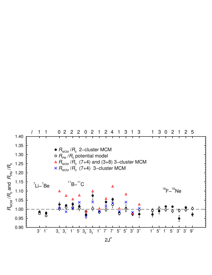
Figure 2: Ratio of the potential model estimate ${\cal R}_{PM}$ to the analytical estimate ${\cal R}_{0}$ (open circles) and ratio of the MCM predictions ${\cal R}_{MCM}$ to the analytical estimate ${\cal R}_{0}$ calculated in the two-cluster (filled circles) and three-cluster microscopic cluster model in which both the ⁷Li+$\alpha$ (⁷Be+$\alpha$) and t+⁸Be (³He+⁸Be) (triangles) or only the ⁷Li+$\alpha$ (⁷Be+$\alpha$) partitions (crosses) have been taken into account.

In Fig.1 we show the deviations $\Delta_{i}$ from $C_{l}^{(2)}$ defined as

$$\Delta_{i}=-\frac{2\mu}{\hbar^{2}}R_{i}(a)/C_{l}^{(2)}$$ (29)

where $i$ = $C$, ${\Delta\Psi}$, ${\delta\phi}$, ${B}$ and $\Delta V_{C}$, together with the total deviation $\Delta=\sum_{i}\Delta_{i}$ for three mirror pairs, ⁷Li(=$\alpha$+t) - ⁷Be(=$\alpha$+${}^{3}He$), ¹¹B(=$\alpha$+⁷Li) - ¹¹C(=$\alpha$+⁷Be) and ¹⁹F(=$\alpha$+¹⁵N) - ¹⁹Ne(=$\alpha$+¹⁵O). The calculations have been done using a Woods-Saxon potential with a diffuseness of 0.65 fm, the radius and the depth of which has been adjusted to fit the $\alpha$-particle energies in mirror systems. The total spin-parity in all three cases is $\frac{3}{2}^{-}$ (the second $\frac{3}{2}^{-}$ state was considered for ¹¹B-¹¹C to enhance the difference in the mirror wave functions) but the orbital momenta $l$ and the number of nodes are different. The ratio $A_{0}(a)/A_{0}(a_{m})$, shown in insets of Fig.1, does not change much near $R_{N}$. The total deviation $\Delta$ is minimal at $r=R_{N}$ and is determined mainly by $\Delta_{\delta\phi}$ when $r<R_{N}$ and by $\Delta_{C}+\Delta_{B}$ at $r>R_{N}$ with $\Delta_{C}$ significantly larger than $\Delta_{B}$. The contribution from $\Delta_{\Delta_{V_{C}}}$ is too small to be shown in these figures.

We have performed exact two-body calculations for other states of the mirror pairs ⁷Li-⁷Be, ¹¹B-¹¹C and ¹⁹F-¹⁹Ne using Woods-Saxon potentials with diffusseness varying from 0.35 to 0.95 fm. The sensitivity of the ratio ${\cal R}$ to the potential choice was less than 2$\%$. Both the exact ratios ${\cal R}_{PM}$ and the analytical approximations ${\cal R}_{0}$ are given in Table I. Since in all cases $a_{m}$ was very close to $R_{N}$ and $A_{0}(a)$ changed very slowly around $R_{N}$, the ${\cal R}_{0}$ values from Table II were calculated at $R_{N}=a_{m}$. The ratio ${\cal R}_{PM}/{\cal R}_{0}$ is also plotted in Fig.2. One can see that ${\cal R}_{PM}$ and ${\cal R}_{0}$ agree on average within 2$\%$ or less. For ⁷Li-⁷Be this agreement is slightly worse, about 3-4$\%$, which can be explained by the larger difference in internal wave functions due to the smaller Coulomb interaction.

Table 1: Microscopic calculations for ${\cal R}_{MCM}$, analytical estimate ${\cal R}_{0}$ and the potential model estimate ${\cal R}_{PM}$, for the mirror pairs from the first column with the spin-parity $J^{\pi}$ and the orbital momentum $l$ of the $\alpha$ particle. Also shown are the ratios ${\cal R}_{b_{\alpha}}^{MCM}=(b_{\alpha}(2)/b_{\alpha}(1))^{2}$, where $b_{\alpha}(i)=C_{\alpha}(i)/\sqrt{S_{\alpha}(i)}$ is the normalized ANC for the nucleus $i$, and $S_{\alpha}$ is the spectroscopic factor. The significance of these ratios is discussed in the text. For ${\cal R}_{MCM}$ and ${\cal R}_{b_{\alpha}}^{MCM}$, average values and range of variations between calculations with V2 and MN potentials and two different oscillator radii are presented. ${\cal R}_{PM}$ is averaged over the choice of different parameters of the Woods-Saxon potentials and shown together with the range of its variation.

Mirror pair	$J^{\pi}$	$l$	${\cal R}_{MCM}$	${\cal R}_{0}$	${\cal R}_{PM}$	${\cal R}_{b_{\alpha}}^{MCM}$
${}^{7}{\rm Li}-^{7}{\rm Be}$	$\frac{3}{2}^{-}$	1	1.35 $\pm$ 0.01	1.37	1.34 $\pm$ 0.01	1.37 $\pm$ 0.01
	$\frac{1}{2}^{-}$	1	1.43 $\pm$ 0.01	1.47	1.41 $\pm$ 0.01	1.45 $\pm$ 0.01
${}^{11}{\rm B}-^{11}{\rm C}$	$\frac{3}{2}^{-}_{1}$	0	1.60 $\pm$ 0.02	1.56	1.57 $\pm$ 0.02	1.55 $\pm$ 0.01
two-cluster MCM		2	1.50 $\pm$ 0.01	1.46	1.49 $\pm$ 0.02	1.51 $\pm$ 0.02
	$\frac{1}{2}^{-}$	2	1.65 $\pm$ 0.02	1.60	1.61 $\pm$ 0.02	1.64 $\pm$ 0.02
	$\frac{5}{2}^{-}$	2	1.85 $\pm$ 0.02	1.82	1.83 $\pm$ 0.02	1.83 $\pm$ 0.02
	$\frac{3}{2}^{-}_{2}$	0	2.23 $\pm$ 0.05	2.30	2.27 $\pm$ 0.02	2.27 $\pm$ 0.02
		2	2.16 $\pm$ 0.05	2.01	2.02 $\pm$ 0.03	2.06 $\pm$ 0.02
	$\frac{1}{2}^{+}$	1	4.55 $\pm$ 0.01	4.61	4.54 $\pm$ 0.04	4.54 $\pm$ 0.02
	$\frac{7}{2}^{-}$	2	4.38 $\pm$ 0.06	4.20	4.19 $\pm$ 0.05	4.24 $\pm$ 0.02
		4	2.51 $\pm$ 0.02	2.38	2.44 $\pm$ 0.04	2.48 $\pm$ 0.01
	$\frac{5}{2}^{+}$	1	13.29 $\pm$ 0.12	13.53	13.19 $\pm$ 0.10	13.2 $\pm$ 0.1
		3	7.79 $\pm$ 0.15	7.75	7.76 $\pm$ 0.10	7.56 $\pm$ 0.04
	$\frac{3}{2}^{+}$	1	$(1.68\pm 0.02)\times 10^{12}$	$1.72\times 10^{12}$	$(1.68\pm 0.02)\times 10^{12}$	$(1.66\pm 0.02)\times 10^{12}$
		3	$(3.59\pm 0.07)\times 10^{11}$	$3.69\times 10^{11}$	$(3.68\pm 0.03)\times 10^{11}$	$(3.55\pm 0.05)\times 10^{11}$
${}^{11}{\rm B}-^{11}{\rm C}$	$\frac{3}{2}^{-}_{1}$	0	1.71	1.56	1.56 $\pm$ 0.02	1.66
three-cluster MCM		2	1.58	1.47	1.49 $\pm$ 0.02	1.56
	$\frac{1}{2}^{-}$	2	1.69	1.60	1.61 $\pm$ 0.02	1.66
	$\frac{5}{2}^{-}$	2	1.96	1.82	1.83 $\pm$ 0.02	1.91
	$\frac{3}{2}^{-}_{2}$	0	2.27	2.30	2.27 $\pm$ 0.02	2.31
		2	2.21	2.01	2.02 $\pm$ 0.03	2.09
	$\frac{1}{2}^{+}$	1	4.63	4.61	4.54 $\pm$ 0.04	4.61
	$\frac{7}{2}^{-}$	2	4.45	4.20	4.19 $\pm$ 0.05	4.24
		4	2.68	2.38	2.44 $\pm$ 0.04	2.64
	$\frac{5}{2}^{+}$	1	13.60	13.53	13.19 $\pm$ 0.10	13.46
		3	8.39	7.75	7.76 $\pm$ 0.10	7.76
	$\frac{3}{2}^{+}$	1	$1.68\times 10^{12}$	$1.72\times 10^{12}$	$(1.68\pm 0.02)\times 10^{12}$	$1.70\times 10^{12}$
		3	$3.79\times 10^{11}$	$3.69\times 10^{11}$	$(3.68\pm 0.03)\times 10^{11}$	$3.69\times 10^{11}$
${}^{19}{\rm F}-^{19}{\rm Ne}$	$\frac{1}{2}^{+}$	1	4.12 $\pm$ 0.06	4.24	4.21 $\pm$ 0.06	4.17 $\pm$ 0.04
	$\frac{5}{2}^{+}$	3	4.23 $\pm$ 0.07	4.27	4.29 $\pm$ 0.04	4.26 $\pm$ 0.07
	$\frac{1}{2}^{-}$	0	4.70 $\pm$ 0.01	4.63	4.61 $\pm$ 0.04	4.66 $\pm$ 0.01
	$\frac{5}{2}^{-}$	2	9.58 $\pm$ 0.04	9.44	9.43 $\pm$ 0.09	9.53 $\pm$ 0.02
	$\frac{3}{2}^{-}$	2	10.74 $\pm$ 0.04	10.63	10.6 $\pm$ 0.1	10.69 $\pm$ 0.03
	$\frac{3}{2}^{+}$	1	8.39 $\pm$ 0.15	8.84	8.78 $\pm$ 0.08	8.56 $\pm$ 0.07
	$\frac{9}{2}^{+}$	5	222 $\pm$ 3	228	229 $\pm$ 2	223 $\pm$ 2

II.2 Mirror ANCs in a microscopic cluster model

The relation (27) for mirror ANCs obtained in the two-body model can be extended to many-body systems. The expression for an ANC in the many-body case is Tim98

$$C^{(i)}_{l}=-\frac{2\mu}{\hbar^{2}}\int_{0}^{\infty}dr\,r^{2}\tilde{\phi}_{l}^{(i)}(r)\,\langle[\Phi_{X_{i}}^{J_{X_{i}}}\otimes Y_{l}(\hat{r})]_{J_{A}}$$

$$\times\Phi_{\alpha}||V_{N}+V_{C_{i}}-\tilde{V}_{i}||\Psi_{A}^{J_{A}}\rangle$$ (30)

where $\Psi_{A}^{J_{A}}$, $\Phi_{\alpha}$ and $\Phi_{X_{i}}^{J_{X_{i}}}$ are the many-body wave functions of the nucleus $A$, $\alpha$-particle and the decay product $X_{i}$, and $J_{A}$ and $J_{X_{i}}$ are the total spins of $A$ and $X_{i}$. The integration in the source term $\langle[\Phi_{X_{i}}^{J_{X_{i}}}\otimes Y_{l}(\hat{r})]_{J_{A}}\Phi_{\alpha}||V_{N}+V_{C_{i}}-\tilde{V}_{i}||\Psi_{A}^{J_{A}}\rangle$ is carried out over the internal coordinates of $\alpha$ and $X_{i}$ and the potentials $V_{N}$ and $V_{C}$ are the sums of the two-body nuclear and Coulomb interactions. Following the reasoning of section A, we get the formula (27). The deviation from this formula will be determined by the remainder terms $R_{C}(a)$, $R_{\Delta\Psi}$, $R_{B}(a)$, $R_{\delta\phi}(a)$ and $R_{\Delta V_{C}}(a)$ defined by Eqs. similar to (15), (19), (20), (21) and (24) but in the integrands of which $V\Psi$ is be replaced by the matrix elements of the $\langle[\Phi_{X_{i}}^{J_{X_{i}}}\otimes Y_{l}(\hat{r})]_{J_{A}}\Phi_{\alpha}||V||\Psi_{A}^{J_{A}}\rangle$ type.

The main difference between the two-body and many-body cases is that $V_{C}-V_{C_{0}}$ is not zero at $r>R_{N}$. It contains long range contributions from the $r^{-\lambda}$ ($\lambda\geq 2$) terms the strengths of which are determined by the matrix elements $\langle[\Phi_{X_{i}}^{J_{X_{i}}}\otimes Y_{l}(\hat{r})]_{J_{A}}\Phi_{\alpha}||M(E\lambda)||\Psi_{A}^{J_{A}}\rangle$ where $M(E\lambda)$ is the electromagnetic operator of multipolarity $\lambda$ Tim05a . If these matrix elements are large, then all the remnant terms that contain $\Delta V_{C_{i}}$ may cause significant differences between ${\cal R}$ and ${\cal R}_{0}$. This is expected for nuclei with strongly deformed and/or easily excited cores.

Another factor that may lead to additional differences between ${\cal R}$ and ${\cal R}_{0}$ in many-nucleon systems is that the condition $\Psi_{l}^{(1)}\approx\Psi_{l}^{(2)}$ for the validity of Eq. (27) in the two-body case is replaced by the equality of the projections $\langle[\Phi_{X_{i}}^{J_{X_{i}}}\otimes Y_{l}(\hat{r})]_{J_{A}}\Phi_{\alpha}|\Psi_{A}^{J_{A}}\rangle$ (or overlap integrals) of the mirror wave functions for nuclei ${}^{A}_{N}Z$ and ${}^{A}_{Z}N$ into the mirror channels $X_{i}+\alpha$. If the norms of these overlap integrals (or spectroscopic factors) differ then the terms $R_{\Delta\Psi}$, $R_{\delta\phi}(a)$ and $R_{\Delta V_{C}}(a)$ will increase. This can be especially important for weak components of overlap integrals where symmetry breaking in the spectroscopic factors may become large.

Our previous study of many-body effects in mirror virtual nucleon decays suggests that they are on average of the order of 7$\%$ Tim05a , although stronger deviations in some individual cases were observed as well. Here, we study the many-body effects in mirror $\alpha$-particle ANCs using a multi-cluster model of the same type as in Ref. Tim05a for the same mirror pairs ⁷Li-⁷Be, ¹¹B-¹¹C and ¹⁹F-¹⁹Ne considered above in the two-body model.

The multi-channel cluster wave function for a nucleus $A$ consisting of a core $X$ and an $\alpha$-particle can be represented as follows:

$$\Psi_{A}^{J_{A}M_{A}}=\sum_{l\omega J_{X}}{\cal A}\,\Phi_{\alpha}\left[g^{J_{X}J_{A}}_{\omega l}(\mbox{\boldmath$r$})\otimes\Phi_{X}^{J_{X}}\right]_{J_{A}M_{A}}$$ (31)

where ${\cal A}$ is the antisymmetrization operator which permutes nucleons between the $\alpha$-particle and the core. Both the $\alpha$-particle wave function and the “core” wave function $\Phi_{X}^{J_{X}}$ corresponding to the total spin $J_{X}$ are defined in the translation-invariant harmonic-oscillator shell model. In addition, for ¹¹C we used the three-cluster model of Ref. Des95 in which $\Phi_{X}^{J_{X}}$ is defined in a two-cluster model. The quantum number $l$ labels the orbital momentum of the $\alpha$-particle. The relative wave function $g^{J_{X}J_{A}}_{\omega lm}(\mbox{\boldmath$r$})=g^{J_{X}J_{A}}_{\omega l}(r)Y_{lm}(\hat{\mbox{\boldmath$r$}})$ is determined using the microscopic R-matrix method Des90 to provide the correct asymptotic behaviour

$$g^{J_{X}J_{A}}_{\omega l}(r)\approx C_{l,\omega}^{J_{X}J_{A}}\frac{W_{-\eta,l+1/2}(2\kappa r)}{r},\,\,\,\,\,\,r\rightarrow\infty,$$ (32)

determined by the Whittaker function and the ANC $C_{l,\omega}^{J_{X}J_{A}}$.

Table 2: The range of changes in squared ANCs $C^{2}_{\alpha}(2)$ and $C^{2}_{\alpha}(1)$ (in fm^-1) for mirror nuclei 2 and 1 ($Z_{2}>Z_{1}$) and in their ratio ${\cal R}_{MCM}$ with the choice of oscillator radius and the NN potential. For ¹¹B - ¹¹C, this range include also changes with different number of clusters. Also shown are the spectroscopic factors $S_{\alpha}(2)$, $S_{\alpha}(1)$ and their ratio ${\cal R}_{S}^{MCM}=S_{\alpha}(2)/S_{\alpha}(1)$.

$J^{\pi}$	$l$	$C^{2}_{\alpha}(2)$	$C^{2}_{\alpha}(1)$	${\cal R}_{MCM}$	$S_{\alpha}(2)$	$S_{\alpha}(1)$	${\cal R}_{S}^{MCM}$
${}^{7}{\rm Li}-^{7}{\rm Be}$
$3/2^{-}$	1	19.4-30.4	14.3-22.6	$1.35\pm 0.01$	1.13-1.15	1.14-1.16	0.99-1.00
$1/2^{-}$	1	14.9-22.7	10.4-16.0	$1.43\pm 0.01$	1.12-1.14	1.13-1.15	0.99
${}^{11}{\rm B}-^{11}{\rm C}$
$3/2^{-}_{1}$	0	(0.54-2.15)$\times 10^{4}$	(0.34-1.25)$\times 10^{4}$	$1.65\pm 0.07$	0.29-0.38	0.28-0.37	1.02-1.03
	2	(1.69-6.74)$\times 10^{3}$	(1.12-4.26)$\times 10^{3}$	$1.54\pm 0.05$	0.45-0.51	0.44-0.51	1.00-1.01
$1/2^{-}$	2	(0.69-3.69)$\times 10^{3}$	(0.42-2.19)$\times 10^{3}$	$1.66\pm 0.03$	0.37-0.42	0.37-0.41	1.00-1.01
$5/2^{-}$	2	(0.51-2.19)$\times 10^{3}$	(0.28-1.12)$\times 10^{3}$	$1.90\pm 0.07$	0.64-0.76	0.64-0.75	1.01-1.02
$3/2^{-}_{2}$	0	(0.76-1.40)$\times 10^{3}$	338-612	$2.25\pm 0.04$	0.09-0.15	0.09-0.15	0.98-1.00
	2	41.9-428	19.4-191	$2.18\pm 0.06$	0.1-0.23	0.09-0.22	1.04-1.06
$1/2^{+}$	1	(0.47-3.00)$\times 10^{4}$	(1.04-6.41)$\times 10^{3}$	$4.59\pm 0.05$	0.66-0.88	0.66-0.87	1.00-1.01
$7/2^{-}$	2	4.67-20.8	1.08-4.67	$4.39\pm 0.07$	0.014-0.026	0.013-0.025	1.03-1.05
	4	0.20-0.75	0.08-0.30	$2.59\pm 0.10$	0.07-0.34	0.06-0.33	1.01-1.02
$5/2^{+}$	1	(1.0-5.0)$\times 10^{4}$	(0.75-3.68)$\times 10^{3}$	$13.4\pm 0.2$	0.84-0.95	0.83-0.94	1.00-1.01
	3	13.3-243	1.72-28.9	$8.03\pm 0.36$	0.034-0.064	0.033-0.059	1.01-1.08
$3/2^{+}$	1	(0.30-1.2)$\times 10^{15}$	179-703	$(1.68\pm 0.02)\times 10^{12}$	0.16-0.38	0.16-0.38	1.00-1.01
	3	(0.09-1.67)$\times 10^{13}$	2.47-44.1	$(3.60\pm 0.07)\times 10^{11}$	0.094-0.18	0.093-0.18	1.00-1.03
${}^{19}{\rm F}-^{19}{\rm Ne}$
$1/2^{+}$	1	(0.42-1.24)$\times 10^{7}$	(1.04-3.00)$\times 10^{6}$	$4.12\pm 0.06$	0.17-0.55	0.17-0.56	0.98-1.00
$5/2^{+}$	3	(2.39-7.97)$\times 10^{5}$	(0.57-1.89)$\times 10^{5}$	$4.23\pm 0.07$	0.15-0.41	0.16-0.42	0.98-1.00
$1/2^{-}$	0	(1.38-5.07)$\times 10^{7}$	(0.30-1.08)$\times 10^{7}$	$4.69\pm 0.02$	0.42-0.69	0.42-0.69	1.00-1.01
$5/2^{-}$	2	(0.71-2.81)$\times 10^{7}$	(0.75-2.92)$\times 10^{6}$	$9.58\pm 0.04$	0.42-0.68	0.41-0.67	1.00-1.01
$3/2^{+}$	1	(1.34-4.59)$\times 10^{7}$	(1.63-5.38)$\times 10^{6}$	$8.39\pm 0.15$	0.17-0.67	0.18-0.68	0.97-0.99
$3/2^{-}$	2	(0.88-3.43)$\times 10^{7}$	(0.82-3.18)$\times 10^{6}$	$10.74\pm 0.04$	0.44-0.69	0.44-0.69	1.00-1.01
$9/2^{+}$	5	(1.31-6.39)$\times 10^{5}$	(0.60-2.87$\times 10^{3}$	$222\pm 3$	0.16-0.30	0.16-0.30	0.99

The MCM requires some choice of the oscillator radius $b$ to describe the internal structure of the clusters. In all three mirror pairs considered in this paper, the oscillator radius that provides a good description of the $\alpha$-particle differs significantly from that of the core. Dealing with different $b$ for each of the cluster would create big difficulties in using the MCM. Therefore, we use the same value of $b$ for both clusters but do the calculations twice. The first time we use $b$ = 1.36 fm that reproduces the r.m.s. radius of the $\alpha$-particle and minimises its binding energy, and the second time we use either $b$ = 1.5 fm (to describe the triton and/or ³He core for the ⁷Li - ⁷Be mirror pair) or $b$ = 1.6 fm (for ¹¹B - ¹¹C and ¹⁹F - ¹⁹Ne). Our previous calculations for ¹⁷O - ¹⁷F have shown that different oscillator radii change strongly the absolute value of neutron and proton ANCs but does not change their ratio very much Tim05a . In the three-cluster calculations for the ¹¹B - ¹¹C mirror pair we used only one value of the oscillator radius, $b$ = 1.36 fm, the same as in Ref. Des95 .

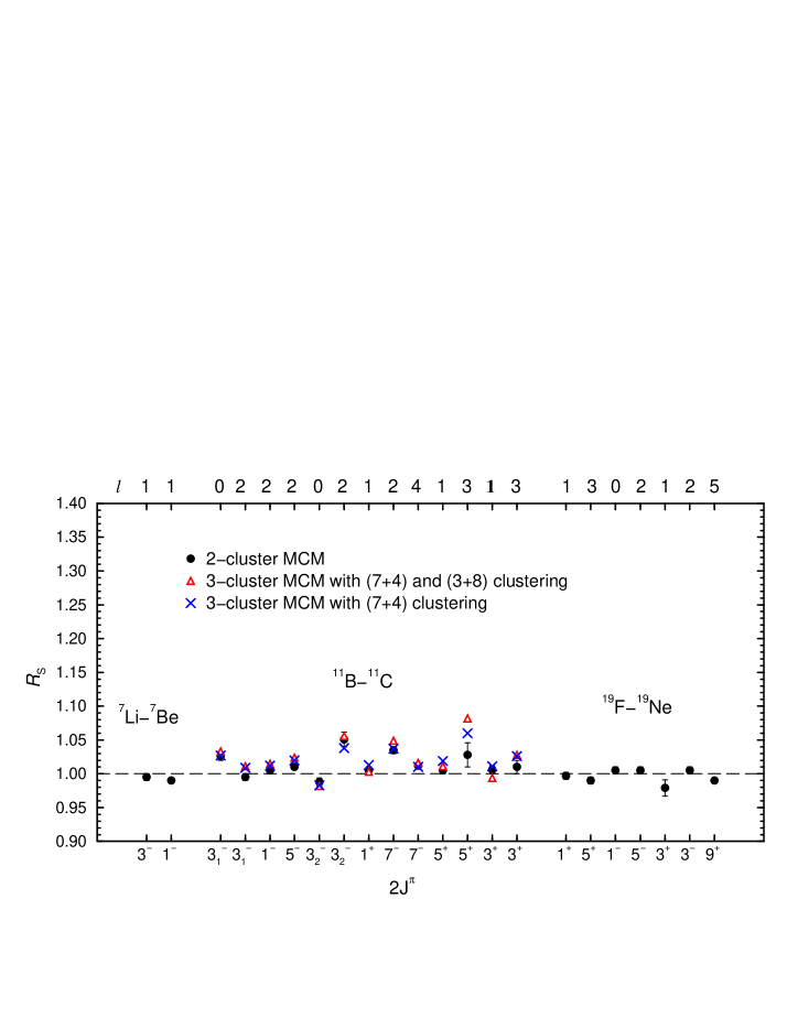
Figure 3: Ratio ${\cal R}_{S}$ of the $\alpha$-particle spectroscopic factors in the ⁷Li-⁷Be, ¹¹B-¹¹C and ¹⁹F-¹⁹Ne mirror pairs, calculated in the two-cluster (filled circles) and three-cluster microscopic cluster models in which both the ⁷Li+$\alpha$ (⁷Be+$\alpha$) and t+⁸Be (³He+⁸Be) (triangles) or only the ⁷Li+$\alpha$ (⁷Be+$\alpha$) partitions (crosses) have been taken into account.

For each oscillator radius, we use two NN potentials, the Volkov potential V2 volkov and the Minnesota (MN) potential minnesota , except in three-cluster calculations for ¹¹B-¹¹C where only V2 is used. The two-body spin-orbit force BP81 with $S_{0}$ = 30 MeV$\cdot$fm⁵ and the Coulomb interaction are also included. Both V2 and MN have one adjustable parameter that gives the strength of the odd NN potentials $V_{11}$ and $V_{33}$. We fit this parameter in each case to reproduce the experimental values for the $\alpha$-particle separation energies. Slightly different adjustable parameters in mirror nuclei, needed to reproduce these energies, simulate charge symmetry breaking of the effective NN interactions, which could be a consequence of charge symmetry breaking in realistic NN interactions.

The range of changes in squared ANCs $C_{\alpha}^{2}(2)$ and $C_{\alpha}^{2}(1)$ in mirror nuclei 2 and 1 is given in Table II. Similar to previous studies of of one-nucleon ANCs in Refs. BT92 ; Tim05a ; Tim06a , the V2 potential gives larger $C_{\alpha}^{2}$ values than the MN (up to a factor of two) at a fixed oscillator radius $b$ and the different choices of $b$ give a comparable change (up to the factor of two) in $C_{\alpha}^{2}$ at a fixed NN potential. The range of change in the ratio ${\cal R}_{MCM}$ with different choices of oscillator radius and the NN potential are also given in Table II. For ¹¹B - ¹¹C, this range includes changes with different number of clusters. In Table I the average value of ${\cal R}_{MCM}$ is compared to the analytical estimate ${\cal R}_{0}$ and to predictions within the potential model ${\cal R}_{PM}$. To visualise the deviation between ${\cal R}_{MCM}$ and ${\cal R}_{0}$ we plot the ratio ${\cal R}_{MCM}/{\cal R}_{0}$ in Fig.2.

We have also calculated the $\alpha$-particle spectroscopic factors $S_{\alpha}$ defined as

$$S_{\alpha}=\left(\begin{array}[]{c}A\\ 4\end{array}\right)\int_{0}^{\infty}dr\,r^{2}\left|\langle[\Phi_{X_{i}}^{J_{X_{i}}}\otimes Y_{l}(\hat{r})]_{J_{A}}\Phi_{\alpha}|\Psi_{A}^{J_{A}}\rangle\right|^{2}$$ (35)

(36)

and have shown their range of variation in Table II. The ratio ${\cal R}_{S}^{MCM}=S_{\alpha}(2)/S_{\alpha}(1)$ of these spectroscopic factors is given in Table II as well and is plotted in Fig.3. We also calculate the ratio ${\cal R}_{b_{\alpha}}^{MCM}=(b_{\alpha}(2)/b_{\alpha}(1))^{2}$ of the normalized squared ANCs $b_{\alpha}=C_{\alpha}/\sqrt{S_{\alpha}}$. As in the case of mirror virtual nucleon decays studied in Ref. Tim05a ; Tim06b , the approximate equality ${\cal R}_{b_{\alpha}}^{MCM}\approx{\cal R}_{PM}$ means that in mirror nuclei the effective local nuclear $\alpha$-core interaction can be considered to be the same.

We now discuss individual mirror pairs in more details.

⁷Li - ⁷Be. The squared ANCs in these mirror nuclei change by about 55$\%$ with different oscillator radii and NN potentials. However, the ratio $C_{\alpha}(^{7}$Be$)/C_{\alpha}(^{7}$Li) changes by only about 1.5$\%$ both in the ground and the first excited states. This ratio differs from the analytical estimate ${\cal R}_{0}$ by no more than 3$\%$ and 4$\%$ for the ground and the first excited state respectively and agrees reasonably well with the potential model calculations. The mirror symmetry in spectroscopic factors is also clearly seen. Some minor differences in ${\cal R}_{b_{\alpha}}^{MCM}$ and ${\cal R}_{PM}$ are present which means that the effective local nuclear $t+\alpha$ and ³He + $\alpha$ interactions differ slightly. Since the ⁷Li and ⁷Be ANCs determine the cross sections for the ³H($\alpha,\gamma$)⁷Li and ³He($\alpha,\gamma$)⁷Be capture reactions at zero energies, the mirror symmetry of the $\alpha$-particle ANCs means that relations should exist between the astrophysical $S$-factors of these reactions. Thus, with our value of ${\cal R}_{MCM}$ the ratio $S_{34}(^{7}$Be$)/S_{34}(^{7}$Li) at zero energy is 6.6 and 5.9 for the ground and the first excited states respectively.

¹¹B - ¹¹C. The calculations for this mirror pair have been performed for all excited states that are below the $\alpha$-particle emission threshold in ¹¹C. In the two-cluster model, only the ground and the $\frac{1}{2}^{-}$ first excited state in the ⁷Li - ⁷Be mirror cores have been taken into account. In the three-cluster model, both the ⁷Li+$\alpha$ (⁷Be+$\alpha$) and t+⁸Be (³He+⁸Be) partitions are taken into account with the first excited states $\frac{1}{2}^{-}$,$\frac{3}{2}^{-}$,$\frac{5}{2}^{-}$ and $\frac{7}{2}^{-}$ in ⁷Li (⁷Be) and the first 0⁺ and 2⁺ states in ⁸Be included Des95 .

The squared ANCs calculated in the two-cluster MCM change with different NN potential and oscillator radius choice by the factor of four on average (see Table II). Taking two-cluster nature of ⁷Li and ⁷Be into account in most cases significantly increases ANCs thus increasing the range of their variations with model assumptions. However, in all cases the ratio ${\cal R}_{MCM}$ changes by no more than 9$\%$. The ${\cal R}_{MCM}$ values obtained in the two-cluster model are close to the analytical estimate ${\cal R}_{0}$ and to the potential model prediction ${\cal R}_{PM}$, agreement being within 1-5$\%$ (see Fig.2). For the second $\frac{3}{2}^{-}$ state with $l=2$, a larger deviation from ${\cal R}_{0}$ and ${\cal R}_{PM}$ (5-10$\%$) coincides with larger symmetry breaking in the mirror spectroscopic factors (see Fig.3).

The ${\cal R}_{MCM}$ values obtained in the three-cluster MCM are significantly larger than the predictions of the two-cluster model. This is caused mainly by the influence of the t+⁸Be and ³He+⁸Be channels. When these channels are removed, so that only the ⁷Li+$\alpha$ and ⁷Be+$\alpha$ partitions are left, then both the two-cluster and three-cluster MCM predict very similar results for the ratio ${\cal R}_{MCM}$ (see Fig.2). At the same time, the ratio of mirror spectroscopic factors is not very much influenced by the t+⁸Be (³He+⁸Be) clustering, although for the $\frac{5}{2}^{+}$ state with $l$ = 3 it is slightly reduced. This happens because the effective local $\alpha-^{7}$Li and $\alpha-^{7}$Be interaction differ. This can be seen by comparing the ${\cal R}_{b_{\alpha}}^{MCM}$ obtained in the three-cluster calculations with ${\cal R}_{PM}$. In two-body calculations these quantities agree with each other within the uncertainties of their calculations for most of the mirror states.

¹⁹F - ¹⁹Ne. The two-cluster MCM calculations for this mirror pair have been performed for all excited states that are below the $\alpha$-particle emission threshold in ¹⁹Ne. The mirror cores ¹⁵N - ¹⁵O were considered both in the ground and the first excited state $\frac{3}{2}^{-}$. We have found that different choices of the oscillator radius strongly influence the mixture of the $\alpha$+¹⁵N($\frac{1}{2}^{-}$) and $\alpha$+¹⁵N($\frac{3}{2}^{-}$) configurations in all the states of ¹⁹F, leading to large changes in spectroscopic factors and ANCs. The same is true for the $\alpha$+¹⁵O($\frac{1}{2}^{-}$) and $\alpha$+¹⁵O($\frac{3}{2}^{-}$) configurations in ¹⁹Ne. However, despite the 3-5 times change in squared ANCs, the ratio ${\cal R}_{MCM}$ of mirror squared ANCs changes by less 3.5$\%$. This ratio is close to both the analytical estimate ${\cal R}_{0}$ and the predictions of the potential model ${\cal R}_{PM}$. The deviation between ${\cal R}_{MCM}$ and these estimates does not exceed 5$\%$. The mirror symmetry in spectroscopic factors is also clearly seen. In most cases ${\cal R}_{b}^{MCM}$ and ${\cal R}_{PM}$ agree within uncertainties of their definition which means that mirror symmetry in the effective local $\alpha+^{15}$N and $\alpha+^{15}$O interactions is a good assumption.

III Bound-unbound mirror pairs

Table 3: Range of change for the width $\Gamma_{\alpha}$ (in MeV) of an $\alpha$-particle resonance and for its mirror squared ANC $C^{2}_{\alpha}$ (in fm^-1) with different model parameters. The results of calculation are given both in the potential model and in the MCM.

			Potential model		Microscopic cluster model
Mirror pair	$J^{\pi}$	$l$	$\Gamma_{\alpha}$	$C^{2}_{\alpha}$	$\Gamma_{\alpha}$	$C^{2}_{\alpha}$
${}^{11}{\rm B}-^{11}{\rm C}$	$\frac{3}{2}^{-}_{3}$	0	(2.13 - 3.53) $\times 10^{-3}$	(2.04 - 3.40 ) $\times 10^{6}$	(0.98 - 2.51) $\times 10^{-3}$	(8.91 - 25.3 ) $\times 10^{5}$
		2	(1.20 - 2.44 ) $\times 10^{-4}$	(8.17 - 16.3 ) $\times 10^{4}$	(3.25 - 11.2 ) $\times 10^{-5}$	(2.18 - 8.11 ) $\times 10^{4}$
${}^{19}{\rm F}-^{19}{\rm Ne}$	$\frac{3}{2}^{+}_{2}$	1	(3.95 - 10.2 ) $\times 10^{-10}$	(1.23 - 3.11 ) $\times 10^{23}$	(0.76 - 2.58 ) $\times 10^{-10}$	(2.21 - 7.54 ) $\times 10^{22}$
	$\frac{7}{2}^{-}_{2}$	4	(3.67 - 15.1 ) $\times 10^{-10}$	(4.68 - 18.4 ) $\times 10^{72}$	(0.98 - 3.40 ) $\times 10^{-13}$	(2.54 - 23.8 ) $\times 10^{69}$

The symmetry in mirror $\alpha$-decays can be extended to bound-unbound mirror pairs. As in the case of nucleon decays Tim03 ; Tim05b , such a symmetry would manifest itself as a link between the ANC of the bound $\alpha$-particle state and the width of its analog resonant state. This follows from the possibility to represent the resonance width by an integral similar to (3) and (30). For isolated narrow resonances, the generalization of Eq. (17) of Ref. Tim05b for the two-body $\alpha$-particle case gives the width $\Gamma_{l}^{0}$ as

$$\Gamma_{l}^{0}\approx\frac{2\kappa_{R}}{E_{R}}\left|\int_{0}^{R_{m}}dr\,rF_{l}(\kappa_{R}r)(V_{N}-\Delta V_{C})\Psi_{l}^{BSA}(r)\right|^{2},$$

(37)

where $E_{R}$ is the resonance energy, $k_{R}=\sqrt{2\mu E_{R}/\hbar^{2}}$, $F_{l}$ is the regular Coulomb wave function and $\Psi_{l}^{BSA}$ is a wave function of the $\alpha$-particle resonance in the bound-state approximation. This function has the dimension of a bound-state wave function and is defined and normalized within some channel radius $R_{m}$ taken well outside the range of the $\alpha$-core interaction. The width $\Gamma_{l}^{0}$ defined by Eq. (37) is related to the residue $\gamma_{l}^{2}$ at the R-matrix pole by Lan58 ,

$$\Gamma_{l}^{0}=2\kappa_{R}R_{m}\,\gamma_{l}^{2}/|O_{l}(\kappa_{R}R_{m})|^{2},$$ (38)

where $O_{l}$ is the outgoing Coulomb function. It determines the observable width $\Gamma_{l}$ by

$$\Gamma_{l}=\Gamma_{l}^{0}/(1+\gamma_{l}^{2}S^{\prime}_{l})^{-1},$$ (39)

where $S_{l}={\rm Re}(\kappa_{R}R_{m}O^{\prime}_{l}/O_{l})$ and the derivation is performed with over the energy $E$. For very narrow resonances, such that $\gamma_{l}^{2}S^{\prime}_{l}\ll 1$, the observed width, $\Gamma_{l}$, and the one related to the residue in the R-matrix pole, $\Gamma_{l}^{0}$, are the same. It is for such cases that the analytical expression for the ratio

$${\cal R}_{\Gamma}=\Gamma_{\alpha}/C^{2}_{\alpha}$$ (40)

can be derived. Following the reasoning of Sec. II.A we get the approximate model-independent formula

$${\cal R}_{\Gamma}\approx{\cal R}_{0}^{res}=\frac{\hbar^{2}k_{R}}{\mu}\frac{\varepsilon_{b.s.}}{E_{R}}\left|\frac{F_{l}(k_{R}R_{N})}{F_{l}(i\kappa_{b.s.}R_{N})}\right|^{2}$$ (41)

where $\varepsilon_{b.s.}$ is the binding energy of a bound $\alpha$-particle state and $\kappa_{b.s.}=\sqrt{2\mu\varepsilon_{b.s.}}/\hbar$. As in the case of bound mirror pairs, the difference between ${\cal R}_{0}^{res}$ and the exact value of ${\cal R}_{\Gamma}$ will be determined by remainder terms similar to those given in Eqs. (15), (19), (20), (21) and (24), and their magnitude will depend on how similar are the bound state $\alpha$-particle wave function and its mirror analog $\Psi_{l}^{BSA}$. As for bound mirror pairs, the formula (41) will be more accurate if the function $|F_{l}(k_{R}r)/F_{l}(\kappa_{b.s.}r)|$ varies slowly near $r\approx R_{N}$. This function changes the most slowly near its maximum, at $r=a_{m}$.

Figure 4: The ratios $|F_{l}(k_{R}a)F_{l}(\kappa_{b.s.}a_{m})/F_{l}(\kappa_{b.s.}a)F_{l}(k_{R}a_{m})|$ as a function of $a$.

Table 4: Analytical estimate ${\cal R}_{PM}^{res}$ and the two-body (${\cal R}_{0}^{res}$) and MCM prediction (${\cal R}_{\Gamma}^{MCM}$) for the ratio ${\cal R}_{\Gamma}$ (all in MeV$\cdot$fm) for some mirror states in ¹¹B-¹¹C and ¹⁹F-¹⁹Ne. $\varepsilon_{b.s}$ is the binding energy of a bound $\alpha$-particle state and $E_{R}$ is the resonance energy of its mirror analog while $l$ is the orbital momentum.

Mirror pair	$J^{\pi}$	$\varepsilon_{b.s}$	$E_{R}$	$l$	${\cal R}_{0}^{res}$	${\cal R}_{PM}^{res}$	${\cal R}_{\Gamma}^{MCM}$
${}^{11}{\rm B}-^{11}{\rm C}$	$\frac{3}{2}^{-}_{3}$	0.104	0.5615	0	$1.18\times 10^{-9}$	$1.05\times 10^{-9}$	(1.05 $\pm$ 0.06) $\times 10^{-9}$
				2	$1.52\times 10^{-9}$	$(1.48\pm 0.01)\times 10^{-9}$	(1.47 $\pm$ 0.03) $\times 10^{-9}$
${}^{19}{\rm F}-^{19}{\rm Ne}$	$\frac{3}{2}^{+}_{2}$	0.1056	0.5038	1	$3.30\times 10^{-33}$	$(3.25\pm 0.04)\times 10^{-33}$	(3.42 $\pm$ 0.04) $\times 10^{-33}$
	$\frac{7}{2}^{-}_{2}$	0.0151	0.6677	4	$7.86\times 10^{-84}$	$(8.00\pm 0.18)\times 10^{-84}$	(1.32 $\pm$ 0.12) $\times 10^{-83}$

In Fig. 4 we plot the function $|F_{l}(k_{R}a)F_{l}(\kappa_{b.s.}a_{m})/$ $F_{l}(\kappa_{b.s.}a)F_{l}(k_{R}a_{m})|$ for three mirror pairs of excited states ¹¹B($\frac{3}{2}^{-}_{3}$, 8.560 MeV) - ¹¹C(($\frac{3}{2}^{-}_{3}$, 8.105 MeV), ¹⁹F($\frac{3}{2}^{+}_{2}$, 3.908 MeV) - ¹⁹Ne($\frac{3}{2}^{+}_{2}$, 4.033 MeV) and ¹⁹F($\frac{7}{2}^{-}_{2}$, 3.999 MeV) - ¹⁹F($\frac{7}{2}^{-}_{2}$, 4.197 MeV). The $\alpha$-particle in the chosen states of ¹¹B and ¹⁹F is weakly bound and its mirror states in ¹¹C and ¹⁹Ne are resonances which are important for some astrophysical applications. This ratio is almost a constant for $r\sim 4-6$ fm which is close to $R_{N}$.

We compare ${\cal R}_{0}^{res}$, calculated assuming $R_{N}=a_{m}$, to ${\cal R}_{\Gamma}$ obtained in exact two-body calculations. To perform the two-body calculations, we have chosen an $\alpha$-core potential of the Woods-Saxon form and varied its diffuseness from 0.35 fm to 0.95 fm. For each diffuseness the depth and the radius of this potential were adjusted to reproduce simultaneously both the $\alpha$-particle separation energy $\varepsilon_{b.s.}$ in a chosen state and the position $E_{R}$ of the resonance in its mirror analog. The width has been determined from the behaviour of the resonant phase shift $\tan\delta_{l}=\Gamma_{l}(E)/2(E-E_{R})$ near $E_{R}$. The range of change in squared ANCs and in resonance widths with the potential geometry is presented in Table III. The widths change by a factor from 1.65 to 4.1 and the ANCs squared in the mirror states change by the same amount so that ${\cal R}_{PM}^{res}$ changes by less than 2$\%$ with respect to an average value. These average values are very close to ${\cal R}_{0}^{res}$ when $l_{\alpha}\neq 0$ (see Table IV). In the $l_{\alpha}=0$ case, when the centrifugal barrier in absent, the approximation (41) becomes less accurate, with ${\cal R}_{PM}^{res}$ being smaller than ${\cal R}_{0}^{res}$ by 12$\%$. This loss of accuracy is probably caused by a larger difference in mirror $s$-wave functions when one of the $\alpha$-particles is loosely-bound. In all cases, the agreement between ${\cal R}_{PM}^{res}$ and ${\cal R}_{0}^{res}$ is much better than for nucleon decays in bound-unbound mirror pairs Tim05b .

To check the validity of the approximation (41) for many-body systems we have calculated ${\cal R}_{\Gamma}$ for bound-unbound mirror states from Tables III and IV using the MCM of the previous section. The width $\Gamma_{\alpha}$ have been calculated by solving the Schrodinger-Bloch equation, as described in Ref. Des90 . The calculations have been done using two oscillator radii for potential V2 and only one oscillator radius, 1.36 fm, for potential MN, because the larger radius, $b$ = 1.6 fm, has caused numerical problems. The resulting ratio ${\cal R}_{\Gamma}^{MCM}$ is presented in Table IV. For ¹¹B($\frac{3}{2}^{+}_{3}$)-¹¹C($\frac{3}{2}^{+}_{3}$) with $l$ = 2 and for ¹⁹F($\frac{3}{2}^{+}_{2}$)-¹⁹Ne($\frac{3}{2}^{+}_{2}$) ${\cal R}_{\Gamma}^{MCM}$ agrees well both with ${\cal R}_{PM}^{res}$ and ${\cal R}_{0}^{res}$. In the case of ¹¹B($\frac{3}{2}^{+}_{3}$)-¹¹C($\frac{3}{2}^{+}_{3}$) with $l_{\alpha}$ = 0 ${\cal R}_{\Gamma}^{MCM}$ agrees only with ${\cal R}_{PM}^{res}$, deviating from ${\cal R}_{PM}^{res}$ by 12$\%$. For ¹⁹F($\frac{7}{2}^{-}_{2}$)-¹⁹Ne($\frac{7}{2}^{-}_{2}$), a 68$\%$ difference between ${\cal R}_{\Gamma}^{MCM}$ and ${\cal R}_{0}^{res}$ is obtained. It originates because of the specific structure of the second $\frac{7}{2}^{-}$ state in ¹⁹F (¹⁹Ne) which is mostly built on the second excited state $\frac{3}{2}^{-}$ of the ¹⁵N (¹⁵O) core with an orbital momentum $l=2$. The spectroscopic factor for the configuration $\langle^{19}$F$|^{15}$O${}_{g.s.}\otimes\alpha\rangle$ is very small, about 10^-3. The spectroscopic factor of the mirror configuration, defined using the concept of the bound state approximation for the narrow resonance function, is also very small. In such weak components effects due to charge symmetry breaking could be large. When the ¹⁵N$(\frac{3}{2}^{-})\otimes\alpha$ (¹⁵O$(\frac{3}{2}^{-})\otimes\alpha$) configuration in ¹⁹F (¹⁹Ne) is neglected, the MCM gives for the $\frac{7}{2}^{-}_{2}$ state ${\cal R}_{\Gamma}^{MCM}$ values that are close both to ${\cal R}_{0}^{res}$ and ${\cal R}_{PM}^{res}$. For example, with V2 and an oscillator radius of 1.6 fm ${\cal R}_{\Gamma}^{MCM}$ = 8.24$\times$10^-84 MeV$\cdot$fm.

IV Unbound mirror pairs

The ideas of Secs. II and III about mirror summetry can be immediately applied to the widths of two mirror narrow resonances 2 and 1. For the ratio

$${\cal R}_{\Gamma\Gamma}=\Gamma_{\alpha}(2)/\Gamma_{\alpha}(1)$$ (42)

Eqs. (27) and (41) can be generalised straightforwardly to give

$${\cal R}_{\Gamma\Gamma}\approx{\cal R}_{\Gamma\Gamma}^{0}=\frac{k_{1}}{k_{2}}\left|\frac{F_{l}(k_{2}R_{N})}{F_{l}(k_{1}R_{N})}\right|^{2},$$ (43)

where $k_{i}=\sqrt{2\mu E_{i}}/\hbar$ and $E_{i}$ is the resonance energy of the $i$-th $\alpha$-particle.

The idea that the widths of two mirror resonances are related has already been used many times to predict unknown widths for those resonances where the widths of their mirror analogs are known. The relation between mirror widths is usually obtained from the relation of the width $\Gamma_{\alpha}$ to the Coulomb barrier penetration factor $P_{l}(E,R_{N})$ and the reduced width $\theta_{\alpha}^{2}$ Lan58 :

$$\Gamma_{\alpha}=\frac{2\hbar^{2}}{\mu R_{N}^{2}}\,\theta_{\alpha}^{2}\,P_{l}(E,R_{N}),$$ (44)

where

$$P_{l}(E,R_{N})=\frac{kR_{N}}{F_{l}^{2}(kR_{N})+G_{l}^{2}(kR_{N})},$$ (45)

$G_{l}^{2}(kR_{N})$ is the irregular Coulomb function, and $R_{N}$ is located somewhere on the surface. Assuming that the reduced widths $\theta_{\alpha}(1)$ and $\theta_{\alpha}(2)$ for mirror resonances are equal one obtains from Eqs.(42), (45) and (44)

$${\cal R}_{\Gamma\Gamma}\approx{\cal R}_{\Gamma\Gamma}^{\theta}\equiv\frac{k_{2}}{k_{1}}\,\frac{F_{l}^{2}(k_{1}R_{N})+G_{l}^{2}(k_{1}R_{N})}{F_{l}^{2}(k_{2}R_{N})+G_{l}^{2}(k_{2}R_{N})}.$$ (46)

The Eqs. (43) and (46) are not identical and can not be deduced one from another.

Figure 5: The ratio $|F_{l}(k_{2}a)/F_{l}(k_{1}a)|$ for $E_{R}(\alpha+^{15}$N) = 0.350 MeV and $E_{R}(\alpha+^{15}$O) = 0.850 MeV for different orbital momenta $l$ as a function of $a$.

Figure 6: The ratio ${\cal R}_{\Gamma\Gamma}^{0}/{\cal R}_{\Gamma\Gamma}^{\theta}$ for different orbital momenta $l$ as a function of the resonance energy $E_{1}$ in $\alpha+^{15}$N.

First, we investigate numerically the difference between the approximations (43) and (46) in a two-body model for a hypothetical mirror pair ¹⁹F - ¹⁹Ne with arbitrary resonance energy $E_{1}$ in the $\alpha+^{15}$N and ($E_{2}$) energy in the ($\alpha+^{15}$O) channel such that $E_{2}=E_{1}+0.5$ MeV, for all $l_{\alpha}\leq 5$. The difference of about 0.5 MeV is typical for low-lying $\alpha$-particle resonances in ¹⁹F - ¹⁹Ne. The ratio $|F_{l}(k_{2}a)/F_{l}(k_{1}a)|$ for such a system is presented in Fig. 5 for the lowest resonance energy in the real $\alpha+^{15}$N system, $E_{1}$ = 0.350 MeV, as a function of $a$. This ratio is varies very slowly for $5<a<8$ fm and reaches its maximum at about 6 - 7 fm, which is beyond the nuclear surface radius $R_{N}$. To compare (43) and (46) we calculate them both at the surface, $R_{N}$ = 5 fm, as has been done in other studies of mirror symmetry in the ¹⁹F - ¹⁹Ne resonances Oli97 ; Dav03 . The ratio ${\cal R}_{\Gamma\Gamma}^{0}/{\cal R}_{\Gamma\Gamma}^{\theta}$ is plotted in Fig.6 for different energies $E_{1}$ taken below the Coulomb barrier. According to Fig.6, ${\cal R}_{\Gamma\Gamma}^{0}$ and ${\cal R}_{\Gamma\Gamma}^{\theta}$ are the same for $E_{1}\leq 2$ MeV but at higher energies a difference appears. This difference increases with decreasing orbital momentum. The largest difference, about 12$\%$, is seen for $l_{\alpha}=0$ at $E_{1}\approx 4$ MeV. The most likely reason for this effect is the growth of the resonance width with the resonance energy. At some point, the integral representation (37) looses its accuracy, making the approxiation (43) invalid. The higher is the centifugal barrier, the higher the resonance energy can be before this happens.

Table 5: Resonance widths $\Gamma_{\alpha}$ for mirror nuclei 1 and 2 (in MeV) and their ratio calculated in the MCM, ${\cal R}_{\Gamma\Gamma}^{MCM}$, and potential model, ${\cal R}_{\Gamma\Gamma}^{PM}$, for mirror states with spin-parity $J^{\pi}$ and orbital momentum $l$.

		Microscopic cluster model			Potential model
$J^{\pi}$	$l$	$\Gamma_{\alpha}(2)$	$\Gamma_{\alpha}(1)$	${\cal R}_{\Gamma\Gamma}^{MCM}$	$\Gamma_{\alpha}(2)$	$\Gamma_{\alpha}(1)$	${\cal R}_{\Gamma\Gamma}^{PM}$
${}^{7}{\rm Li}-^{7}{\rm Be}$
$\frac{7}{2}^{-}_{1}$	3	0.142-0.267	0.079-0.149	1.795 $\pm$ 0.005	0.247	0.134	1.82
${}^{11}{\rm B}-^{11}{\rm C}$ two-cluster MCM
$\frac{5}{2}^{-}_{2}$	2	(1.68-4.21)$\times$10-4	(1.07-2.56)$\times$10-7	1610$\pm$40	6.47$\times$10-3	4.51$\times$10-6	1434
	4	(5.25-26.6)$\times$10-7	(5.28-26.6)$\times$10-7	(1.02$\pm$0.04)$\times$104	7.44$\times$10-5	7.46$\times$10-9	9964
$\frac{7}{2}^{+}_{1}$	3	(2.19-7.20)$\times$10-4	(5.78-18.5)$\times$10-6	38.4 $\pm$ 0.5	6.19$\times$10-3	1.67$\times$10-4	37
	5	(0.82-8.19)$\times$10-8	(0.58-5.18)$\times$10-10	151 $\pm$ 7	5.38$\times$10-5	3.54$\times$10-7	152
${}^{11}{\rm B}-^{11}{\rm C}$ three-cluster MCM
$\frac{5}{2}^{-}_{2}$	2	2.70$\times$10-4	1.55$\times$10-7	1740
	4	1.24$\times$10-6	1.08$\times$10-10	1.14$\times$104
$\frac{7}{2}^{+}_{1}$	3	1.60$\times$10-3	3.95$\times$10-5	40.3
	5	2.11$\times$10-6	1.15$\times$10-8	183
${}^{19}{\rm F}-^{19}{\rm Ne}$
$\frac{7}{2}^{+}_{1}$	3	(0.45-1.95)$\times$10-8	(0.36-1.50)$\times$10-13	(1.28$\pm$0.03)$\times$105	1.23$\times$10-6	9.50$\times$10-12	1.29$\times$105
$\frac{5}{2}^{-}_{2}$	2	(0.89-283)$\times$10-7	(0.48-134)$\times$10-9	204$\pm$7	2.84$\times$10-4	1.40$\times$10-6	203

Next, we compare ${\cal R}_{\Gamma\Gamma}^{0}$ and ${\cal R}_{\Gamma\Gamma}^{\theta}$ to the results of potential model and MCM calculations for some realistic mirror narrow resonances in ⁷Li - ⁷Be, ¹¹B - ¹¹C and ¹⁹F - ¹⁹Ne. Unlike in previous sections, only one value of the diffuseness, 0.65 fm, has been used in the potential model calculations. As for the MCM, the conditions of the calculations are the same as in previous sections.

Table 6: Analytical estimates ${\cal R}_{\Gamma\Gamma}^{\theta}$ and ${\cal R}_{\Gamma\Gamma}^{0}$, MCM ratio ${\cal R}_{\Gamma\Gamma}^{MCM}$, potential model prediction ${\cal R}_{\Gamma\Gamma}^{PM}$ and the ratio ${\cal R}_{\Gamma\Gamma}^{exp}$ of experimentally known widths of mirror states in ⁷Li-⁷Be, ¹¹B-¹¹C and ¹⁹F-¹⁹Ne with spin-parity $J^{\pi}$ and orbital momentum $l$.

Mirror pair	$J^{\pi}$	$E_{1}$	$E_{2}$	$l$	${\cal R}_{\Gamma\Gamma}^{\theta}$	${\cal R}_{\Gamma\Gamma}^{0}$	${\cal R}_{\Gamma\Gamma}^{MCM}$	${\cal R}^{PM}_{\Gamma\Gamma}$	${\cal R}_{\Gamma\Gamma}^{exp}$
${}^{7}{\rm Li}-^{7}{\rm Be}$	$\frac{7}{2}^{-}_{1}$	2.1622	2.983	3	1.74	1.79	1.795 $\pm$ 0.005	1.82	1.88$\pm$0.24
${}^{11}{\rm B}-^{11}{\rm C}$	$\frac{5}{2}^{-}_{2}$	0.2556	0.876	2	1493	1520	1660$\pm$80	1434	2140$\pm$970
				4	9982	1.0$\times$104	(1.06$\pm$0.08)$\times$104	9964
	$\frac{7}{2}^{+}_{2}$	0.5204	1.111	3	38.1	38.3	39.1$\pm$1.2	37.0
				5	152.3	152.2	163$\pm$20	151.8
${}^{19}{\rm F}-^{19}{\rm Ne}$	$\frac{7}{2}^{+}_{1}$	0.364	0.850	3	1.31$\times$105	1.30$\times$105	(1.28$\pm$0.03)$\times$105	1.29$\times$105
	$\frac{5}{2}^{-}_{2}$	0.6692	1.1826	2	209	207	204$\pm$7	203	121$\pm$55

The calculated widths $\Gamma_{\alpha}$ in mirror resonances and their ratio are presented in Table V. In Table VI these ratios are compared to ${\cal R}_{\Gamma\Gamma}^{0}$ and ${\cal R}_{\Gamma\Gamma}^{\theta}$. In all cases studied, $\Gamma_{\alpha}$ depends strongly on the choice of the model and its parameters. For the ⁷Li-⁷Be and ¹⁹F-¹⁹Ne mirror pairs, the ratios ${\cal R}_{\Gamma\Gamma}^{MCM}$ and ${\cal R}_{\Gamma\Gamma}^{PM}$ agree very well with the analytical predictions ${\cal R}_{\Gamma\Gamma}^{0}$ and ${\cal R}_{\Gamma\Gamma}^{\theta}$. For ⁷Li-⁷Be they also agree with experimental value ${\cal R}_{\Gamma\Gamma}^{exp}$ = $\Gamma_{\alpha}^{exp}(^{7}$Be$)/\Gamma_{\alpha}^{exp}(^{7}$Li) obtained using the ⁷Li and ⁷Be widths of the $\frac{7}{2}^{-}$ resonance from Til02 . For the $\frac{5}{2}^{-}_{2}$ resonance in ¹⁹F-¹⁹Ne, the value ${\cal R}_{\Gamma\Gamma}^{exp}$ = 121 $\pm$ 55 determined by using $\Gamma_{\alpha}^{exp}$ from Dav03 is much smaller than the theoretical values of 203 - 211. The most likely reason for this is that the ¹⁹Ne($\frac{5}{2}^{-}_{2}$) width has been determined Ref. Dav03 indirectly using the measured ¹⁹Ne($\frac{5}{2}^{-}_{2}$) branching ratio $\Gamma_{\alpha}/\Gamma$ and its $\gamma$-width assuming that $\Gamma_{\gamma}(^{19}$F) = $\Gamma_{\gamma}(^{19}$Ne). Such an assumption is not always valid.

For ¹¹B-¹¹C, ${\cal R}_{\Gamma\Gamma}^{PM}$ agrees very well with the analytical predictions ${\cal R}_{\Gamma\Gamma}^{0}$ and ${\cal R}_{\Gamma\Gamma}^{\theta}$. The two-cluster MCM predictions also agree with them, expect for the $\frac{5}{2}^{-}_{2}$ state with $l_{\alpha}$ = 2 where a 10$\%$ increase in the ratio of mirror widths can be seen. The three-cluster MCM increases this ratio which could be due to the ⁸Be+t and ⁸Be+³He clustering effects. Both the two- and three-cluster predictions agree with the ratio of experimentally determined widths taken from Ajz90 . In all cases, the difference between the microscopic calculations and the analytical approximations (43) and (46) does not exceed 10$\%$.

V Summary and conclusion

In this paper, we have shown that the structureless two-body bound mirror systems $\alpha+X_{1}$ and $\alpha+X_{2}$, with the same strong nuclear attraction but different Coulomb repulsion, should have ANCs that are related by a model-independent analytical approximation (27). This expression involves the ratio of the regular Coulomb wave functions calculated at imaginary momentum at some distance $a$ between $\alpha$ and $X$. We have demonstrated that if this distance is taken at the point where the product of $\alpha-X$ potential and $\alpha-X$ wave function is the largest, which occurs around $R_{N}\approx(1.1-1.3)(4^{1/3}+X^{1/3})$, then deviation from this approximation should be small provided the nuclear wave functions of these mirror systems are similar to each other in the region that gives most contribution to the ANC in Eq. (3). The analytical approximation (27) remains valid for mirror systems with a many-body internal structure if mirror spectroscopic factors are approximately the same and if $X_{1}$ and $X_{2}$ are not too strongly deformed and/or do not have easily excited low-lying states.

The isospin symmetry between mirror $\alpha$-decays extends to bound-unbound and unbound mirror pairs. In the first case, a link between the $\alpha$-particle ANC of a bound state and the width of its mirror unbound analog is given by the formula (41). In the second case, the link between the widths of mirror resonances can be given by a new formula (43) that at the energies well below the combined Coulomb and centrifugal barrier complements the old formula (46) obtained using the concept of the penetrability of the Coulomb barrier and assuming equality of the reduced widths of mirror resonances.

The comparison of the approximations (27), (41) and (43) to the results of exact calculations either in a two-body potential model or in a microscopic cluster model for three mirror pairs, ⁷Li - ⁷Be, ¹¹B - ¹¹C and ¹⁹F - ¹⁹Ne, have confirmed their validity for many mirror nuclear states. The deviations from these approximations are smaller than those seen in mirror nucleon decays in Ref. Tim05a ; Tim05b because the difference in mirror $\alpha$-particle wave functions are much smaller than the differences in mirror proton and neutron wave functions, especially for loosely-bound states. The largest deviations from analytical estimates have been seen for three-cluster ¹¹B - ¹¹C mirror states with excited ⁷Li and ⁷Be cores. Also, a noticeable deviation has been seen for the second $\frac{7}{2}^{-}$ state in ¹⁹F-¹⁹Ne. This state has tiny spectroscopic factors for the decay channels $\alpha+^{15}$N_g.s. and $\alpha+^{15}$O_g.s. (about 0.001) and the probability of symmetry breaking in such week components is always large.

The ANCs and $\alpha$-widths calculated in our microscopic approach are sensitive to the model assumptions. In particular, they change within a factor of four for different choices of the effective NN potential and oscillator parameters, the smallest values being produced by combiningthe MN potential with the oscillator parameter $b$ = 1.36 fm and the largest values predicted by V2 with $b$ = 1.6 fm. The variation of ANCs and $\alpha$-widths with model assumptions can be even stronger if mirror states have specific structure, for example, the t+⁸Be and ³He+⁸Be configurations in ¹¹B and ¹¹C. However, the calculated in the MCM ratios ${\cal R}$, ${\cal R}_{\Gamma}$ and ${\cal R}_{\Gamma\Gamma}$ do not change much with different choices of unput model parameters. This fact can be used to predict unknown ANCs or $\alpha$-widths if the corresponding mirror quantities have been measured. Such predictions can be beneficial for nuclear astrophysics. Many low-energy $(\alpha,\gamma)$, $(\alpha,N)$ and $(N,\alpha)$ reactions proceed via the population of isolated $\alpha$-particle narrow resonances the widths of which determine the corresponding reaction rates. It is not always possible to measure such widths because of the very small reaction cross sections involved. In this case, using isospin symmetry in mirror $\alpha$-decays may be helpful. For unbound mirror states this symmetry has already been used. For another class of mirror pairs, when the mirror analogs of the resonances are bound, $\alpha$-widths can be determined by measuring the ANCs of bound states in $\alpha$-transfer reactions and using the relation $\Gamma_{\alpha}={\cal R}_{\Gamma}C^{2}_{\alpha}$. As an example, we can point out that the widths of the astrophysically important resonance ¹⁹Ne($\frac{3}{2}^{+}_{2})$ at 4.033 MeV could be detemined if the ANC of its mirror analog in ¹⁹F was known. Unfortunately, available data on the ¹⁵N(⁶Li,d)¹⁹F${}^{*}(\frac{3}{2}_{2}^{+})$ reaction do not allow the extraction the ANC of interest because of strong sensitivity to optical potentials and to the geometry of the bound state potential well that arises due to angular momentum mismatch. An alternative possibility to measure this ANC with a high precision is to use the reaction ¹⁵N(¹⁹F,¹⁵N)¹⁹F^∗. This reaction involves the same optical potentials in the entrance and exit channels and would not suffer the angular momentum mismatch.

VI Appendix

We prove here that $BW_{2}/a\phi_{l}^{(1)}$ is small with respect to $A_{0}(a)$. The coefficients $A$ and $B$ that are found from the continuity of $\tilde{\phi}_{l}^{(2)}(r)$ and its derivative at $r=a$ can alternatively be presented as follows:

$$A=\frac{(W_{2}/a)^{\prime}\phi_{l}^{(2)}-(W_{2}/a)\phi_{l}^{\prime(2)})}{(W_{2}/a)^{\prime}\phi_{l}^{(1)}-(W_{2}/a)\phi_{l}^{\prime(1)}},$$ (47)

$$B=-\frac{\phi_{l}^{\prime(1)}\phi_{l}^{(2)}-\phi_{l}^{(1)}\phi_{l}^{\prime(2)}}{\phi_{l}^{\prime(1)}(W_{2}/a)-\phi_{l}^{(1)}(W_{2}/a)^{\prime}},$$ (48)

where ^′ means differentiation with respect to $a$. When expressed in terms of $F_{1},\,F_{2},\,$ and $W_{2}$ we find

$$B=-\frac{\exp(\imath\delta_{2})}{\kappa_{2}}\frac{F_{2}F_{1}^{\prime}-F_{2}^{\prime}F_{1}}{W_{2}F_{1}^{\prime}-W_{2}^{\prime}F_{1}},$$ (49)

where $\delta_{2}=-(l+1+\imath\eta_{2})\pi/2$. Therefore the quantity $BW_{2}/(a\phi_{l}^{(1)}A_{0}(a))$ is

$$BW_{2}/(a\phi_{l}{(1)}A_{0}(a))=-\frac{F_{1}^{\prime}/F_{1}-F_{2}^{\prime}/F_{2}}{F_{1}^{\prime}/F_{1}-W_{2}^{\prime}/W_{2}}.$$ (50)

We can get a good idea about the magnitude of this term by using semiclassical expressions for the $F_{i}$ and $W_{2}$. For our purposes we can write

$$W_{2}(a)=\frac{W_{2}(b)\exp(-\int_{b}^{a}dr\,p_{2}(r))}{\sqrt{p_{2}(a)/p_{2}(b)}},$$ (51)

$$F_{i}(a)=\frac{F_{i}(b)\exp(+\int_{b}^{a}dr\,p_{i}(r))}{\sqrt{p_{i}(a)/p_{i}(b)}},$$ (52)

where the local wave numbers $p_{i}(r)$ are given by

$$p_{i}(r)=\sqrt{\frac{2\eta_{i}\kappa_{i}}{r}+\frac{l(l+1)}{r^{2}}+\kappa_{i}^{2}},$$ (53)

and $b$ is an arbitrary point in the region where the semiclassical approximation is valid. We also assume that $a$ and $b$ lie in the region where the exponentially decreasing components of the $F_{i}$ can be ignored.

Using these expressions and evaluating the derivatives in a way which consistently respects the semiclassical approximation (see Brink85 , pages 23-24) we find

$$BW_{2}/(a\phi_{l}^{(1)}A_{0}(a))=\frac{p_{2}(a)-p_{1}(a)}{p_{2}(a)+p_{1}(a)}.$$ (54)

For values of $a$ in the nuclear surface the difference $p_{2}(a)-p_{1}(a)$ tends to be very small fraction of $p_{2}(a)+p_{1}(a)$. Note that the condition $p_{1}(a)-p_{2}(a)=0$ is exactly the condition (in the semi-classical approximation) that $A_{0}(a)$ be a stationary function of $a$.

References

- (1) N.K. Timofeyuk, R.C. Johnson and A.M. Mukhamedzhanov, Phys. Rev. Lett. 91, 232501 (2003).
- (2) N.K. Timofeyuk and P. Descouvemont, Phys. Rev. C 71, 064305 (2005).
- (3) N.K. Timofeyuk and P. Descouvemont, Phys. Rev. C 72, 064324 (2005).
- (4) L.Trache, A.Azhari, F.Carstoiu, H.L.Clark, C.A.Gagliardi, Y.-W.Lui, A.M.Mukhamedzhanov, X.Tang, N.Timofeyuk, R.E.Tribble, Phys.Rev. C 67, 062801(R) (2003)
- (5) B. Guo et al, Nucl. Phys. A 761, 162 (2005)
- (6) N.K. Timofeyuk and S.B. Igamov, Nucl. Phys. A713, 217 (2003)
- (7) B. Guo, Z.H. Li, X.X. Bai, W.P. Liu, N.C. Shu, Y.S. Chen, Phys. Pev. C 73, 048801 (2006)
- (8) N.K. Timofeyuk, D.Baye, P.Descouvemont, R. Kamouni and I.J. Thompson, Phys. Rev. Lett. 96, 162501 (2006)
- (9) N.K. Timofeyuk, Nucl. Phys. A 632, 19 (1998)
- (10) P. Descouvemont, Nucl. Phys. A 584, 532 (1995)
- (11) A.B. Volkov, Nucl. Phys. 74, 33 (1965).
- (12) D.R. Thompson, M. LeMere and Y.C. Tang, Nucl. Phys. A286, 53 (1977).
- (13) D. Baye and N. Pecher, Bull Sc. Acad. Roy. Belg. 67 835, (1981).
- (14) D. Baye and N.K. Timofeyuk, Phys. Lett. 293B, 13 (1992)
- (15) N.K. Timofeyuk, P. Descouvemont and R.C. Johnson, Eur. Phys. J. A 27, Suppl. 1, 269 (2006)
- (16) P. Descouvemont and M. Vincke Phys. Rev. A 42, 3835 (1990)
- (17) A.M. Lane and R.G. Thomas, Rev. Mod. Phys. 30, 257 (1958)
- (18) F. de Oliveira et al, Phys. Rev. C 55, R3149 (1997)
- (19) B.Davids, A.M.van den Berg, P.Dendooven, F.Fleurot, M.Hunyadi, M.A.de Huu, R.H.Siemssen, H.W.Wilschut, H.J.Wortche, M.Hernanz, J.Jose, K.E.Rehm, A.H.Wuosmaa, R.E.Segel, Phys.Rev. C 67, 065808 (2003)
- (20) Z.Q. Mao, H.T. Fortune and A.G. Lacaze Phys. Rev. C 53, 1197 (1996).
- (21) D.R. Tilley, C.M. Cheves, J.L. Godwin, G.M. Hale, H.M. Hofmann, J.H. Kelley, C.G. Sheu, H.R. Weller, Nucl. Phys. A 708, 3 (2002)
- (22) F. Ajzenberg-SeloveJ AND J.H. Kelley, Nucl. Phys. A 506, 1 (1990)
- (23) D.M.Brink, Semi-classical Methods in Nucleus-Nucleus Scattering, Cambridge University Press 1985.