Abstract

An approach for calculation of transition form factors of hydrogen-like elementary atoms (EA) is proposed. A general formula for bound-continuous transition form factors of EA is derived. It is shown that these form factors can be represented in the form of finite sum of terms with simple analytical structure and may be numerically evaluated with arbitrary degree of accuracy. As an application of the presented form factors, the calculation of the spectra of products from EA ionization is considered.

1 Introduction

The problem of calculation of transition form factors from bound to unbound states of hydrogen-like atoms [1] has a long history [2-4]. Nowadays, this problem became of great importance for the interpretation of the data of DIRAC experiment at CERN which aims to observe hydrogen-like EA [5] consisting of $\pi^{\pm}$ and/or $\pi^{\mp}$/$K^{\mp}$ mesons (dimesoatoms) and measure the lifetime of $\pi^{+}\pi^{-}$ atoms ($A_{2\pi}$) with accurace of 10% [6-8].

The usual approach to this problem is based on the decomposition of continuum wave functions into infinite series of partial waves and calculation of transition form factors from initial bound state to final continuum state with definite value of angular momentum [4].

In this approach only finite number of terms of infinite series are taken into account in actual calculation leaving unsolved the problem of estimation for contribution of omitted tail with infinite number of terms.

We would like to show in this paper that above mentioned transition (bound to continuum) form factors of hydrogen-like EA may be explicitly calculated without decomposition of final state into infinite series of partial waves.

The plan of the paper is as follows. First of all in Section 2 we shall prove this statement for the simplest case when orbital momentum of bound state is equal zero, i.e. we restrict of ourselves with initial $nS$-states. The generalization of this consideration for the case of arbitrary initial states will be done in Section 3. Finally in Section 4 we compute the spectra of $\pi^{+}\pi^{-}$ pairs from ionization (dissociation) of $A_{2\pi}^{nS}$ as an application of the presented form factors.

2 Transitions from $nS$-states

We define the transition form factors with the help of the following equation:

$$S_{fi}(\vec{q})=\int\psi_{f}^{\ast}(\vec{r})e^{i\vec{q}\vec{r}}\psi_{i}(\vec{r})d^{3}r\,,$$ (1)

where $\psi_{i(f)}$ are the wave functions of initial (final) states of hydrogen-like atoms, $\vec{q}$ is the transferred momentum.

For the case when $i=n00\equiv nS$

$$\psi_{i}=\psi_{n00}(\vec{r}) = \left(\frac{\omega^{3}}{\pi}\right)^{\frac{1}{2}}\exp(-\omega r)\cdot\Phi(-n+1;2;2\omega r)$$ (2)

$$\equiv \left(\frac{\omega^{3}}{\pi}\right)^{\frac{1}{2}}n^{-1}\exp(-\omega r)\cdot L^{1}_{n-1}(2\omega r)\,,$$

where $\omega=\mu\alpha/n$; $\mu$ is the reduced mass and $\alpha=1/137$ is the fine structure constant; $\Phi$ is the confluent hypergeometric function and $L^{\lambda}_{k}$ are the associated Laguerre polynomials.

The wave function of the final (continuum) state must be choose in the form [11]

$$\psi_{f}(\vec{r})=\psi_{\vec{p}}^{(-)} = c^{(-)}\exp(i\vec{p}\vec{r})\cdot\Phi\left[-i\xi,1,-i(pr+\vec{p}\vec{r})\right]\,,$$ (3)

$$c^{(-)}=(2\pi)^{-\frac{3}{2}}\exp\left(\frac{\pi\xi}{2}\right)\Gamma(1+i\xi)\,,$$

$$\xi=\frac{\mu\alpha}{p}\,.$$

Now we use recurrence relation for the Laguerre polynomials [12]

$$L_{k}^{\lambda+1}(x)=\frac{1}{x}\left[(k+\lambda+1)L_{k-1}^{\lambda}(x)-(k+1)L_{k}^{\lambda}(x)\right]$$ (4)

and their representation with the help of the generating function

$$L_{k}^{\lambda}(x)=\Delta_{z}^{(k)}\left[(1-z)^{-(\lambda+1)}\exp\left(\frac{xz}{z-1}\right)\right]\,,$$ (5)

where operator $\Delta_{z}^{(k)}$ is defined as follows:

$$\Delta_{z}^{(k)}\left[f(z)\right]=\frac{1}{k!}\left.\left(\frac{d^{k}}{dz^{k}}f(z)\right)\right|_{z=0}\,.$$ (6)

Then

$$\psi_{i}(r)=\frac{1}{2r}\left(\frac{\omega}{\pi}\right)^{\frac{1}{2}}\left[\Delta_{z}^{(n-1)}-\Delta_{z}^{(n)}\right]\left[(1-z)^{-1}\exp\left[-\omega(z)r\right]\right]\,,$$ (7)

$$\omega(z)=\omega\cdot\frac{1+z}{1-z}\,.$$ (8)

The substitution of Eqs. (42) and (28) to (21) gives

$$S_{\vec{p},noo}(\vec{q})=\frac{1}{2}\left(\frac{\omega}{\pi}\right)^{\frac{1}{2}}c^{(-)}\left[\Delta_{z}^{(n-1)}-\Delta_{z}^{(n)}\right]\left[\frac{J(\vec{q},\vec{p},z)}{(1-z)}\right]\,,$$ (9)

$$J(\vec{q},\vec{p},z)=\int\frac{d^{3}r}{r}\Phi\left[i\xi,1,i(pr+\vec{p}\vec{r})\right]\exp[i(\vec{q}-\vec{p})\vec{r}-\omega(z)r]\,.$$ (10)

The last integral is easily calculated using integral representation for the hypergeometrical functions (see e.g. [14]).

The result reads

$$J(\vec{q},\vec{p},z)=4\pi[\omega^{2}(z)+\vec{\Delta}^{2}]^{-1+i\xi}\left[[\omega(z)-ip]^{2}+q^{2}\right]^{-i\xi}\,,$$ (11)

where $\vec{\Delta}=\vec{q}-\vec{p}$.

Taking into account the definition (29) and obvious the relation

$$\Delta_{z}^{(n)}\left[zf(z)\right]=\Delta_{z}^{(n-1)}f(z)\,,$$ (12)

(9) may be rewritten in the form

$$S_{\vec{p},noo}(\vec{q})=-4(\pi\cdot\omega)^{\frac{1}{2}}c^{(-)}\left(\Delta_{z}^{(n)}-2\Delta_{z}^{(n-1)}+\Delta_{z}^{(n-2)}\right)\left(D_{1}^{-1+i\xi}D_{2}^{-i\xi}\right)\,,$$ (13)

$$D_{1}=(1+z^{2})(\omega^{2}+\vec{\Delta}^{2})-2z(\vec{\Delta}^{2}-\omega^{2})\,,$$

$$D_{2}=(\omega-ip)^{2}+q^{2}-2z(q^{2}-p^{2}-\omega^{2})+z^{2}\left((\omega+ip)^{2}+q^{2}\right)\,.$$

Using the definition of the Gegenbauer polynomials [12, 13]

$$(1-2xz+z)^{-\lambda}=\sum_{k=0}^{\infty}C_{k}^{(\lambda)}(x)\cdot z^{k}\,,$$ (14)

it is easy to obtain

$$D_{1}^{-1+i\xi}=(\Delta^{2}+\omega^{2})^{-1+i\xi}\sum_{k=0}^{\infty}C_{k}^{(1-i\xi)}(u)\cdot z^{k}\,,$$ (15)

$$u=\frac{\Delta^{2}-\omega^{2}}{\Delta^{2}+\omega^{2}}\,;$$

$$D_{2}^{-i\xi}=[(\omega-ip)^{2}+q^{2}]^{-i\xi}\sum_{k=0}^{\infty}C_{k}^{(i\xi)}(v)\cdot w^{k}\cdot z^{k}\,,$$ (16)

$$v=\frac{q^{2}-p^{2}-\omega^{2}}{\sqrt{[(\omega-ip)^{2}+q^{2}][(\omega+ip)^{2}+q^{2}]}}\,,$$

$$w=\sqrt{\frac{(\omega+ip)^{2}+q^{2}}{(\omega-ip)^{2}+q^{2}}}\,.$$ (17)

At least, with the help of the relations

$$\Delta_{z}^{(n)}[f_{1}(z)f_{2}(z)]=\sum_{k=0}^{n}\left[\Delta_{z}^{(n-k)}f_{1}(z)\right]\left[\Delta_{z}^{(k)}f_{2}(z)\right]$$ (18)

and

$$C_{n}^{(\lambda)}(x)-C_{n-1}^{(\lambda)}(x)=\frac{\Gamma(\lambda-\frac{1}{2})\Gamma(n-1+2\lambda)}{\Gamma(2\lambda-1)\Gamma(n+\lambda-\frac{1}{2})}\cdot P_{n}^{(\lambda-\frac{3}{2},\lambda-\frac{1}{2})}(x)\,,$$ (19)

where $P_{n}^{(\lambda-\frac{3}{2},\lambda-\frac{1}{2})}(x)$ are the Jacobi polynomials, we finally obtain

$$S_{\vec{p},noo}(\vec{q})=-2(\pi\cdot\omega)^{\frac{1}{2}}\cdot c^{(-)}\cdot(\omega^{2}+\Delta^{2})^{-1+i\xi}$$ (20)

$$\times[(\omega-ip)^{2}+q^{2}]^{-i\xi}\frac{\Gamma\left(\frac{1}{2}-i\xi\right)}{\Gamma\left(1-2i\xi\right)}\sum_{k=0}^{n}w^{k}C_{k}^{(i\xi)}(v)$$

$$\times\left[\frac{\Gamma\left(n-k+1-2i\xi\right)}{\Gamma\left(n-k+\frac{1}{2}-i\xi\right)}P_{n-k}^{(-\frac{1}{2}-i\xi,\frac{1}{2}-i\xi)}(u)-\frac{\Gamma\left(n-k-2i\xi\right)}{\Gamma\left(n-k-\frac{1}{2}-i\xi\right)}P_{n-k-1}^{(-\frac{1}{2}-i\xi,\frac{1}{2}-i\xi)}(u)\right].$$

Thus, the result of the calculation for transition form factors of hydrogen-like atoms for the case $nS$-continuum transitions is expressed in terms of the classical polynomials and may be easily evaluated numerically with arbitrary degree of accuracy [15].

3 General case

In the previous Section it have been shown that the form factors of transitions from $nS\;(n00)$ - states of hydrogen-like atoms to the state of continuous spectra with definite value of relative momenta $\vec{p}$ may be expressed in the terms of the classical polynomials in a rather simple way. Below this result is generalized for the case of transition from arbitrary initial bound states.

The transition form factors are defined as follows:

$$S_{fi}(\vec{q})=\int\psi_{f}^{\ast}(\vec{r})e^{i\vec{q}\vec{r}}\psi_{i}(\vec{r})d^{3}r\,,$$ (21)

Here, $\psi_{i(f)}$ are the wave functions of initial (final) states.

According to [16] (see also [11]), the final state wave function must be choose in the form

$$\psi_{i}(\vec{r})\equiv\psi_{n00}(\vec{r})\,.$$ (22)

For arbitrary initial bound state

$$\psi_{i}(\vec{r})=\psi_{nlm}(\vec{r})=Y_{lm}\left(\frac{\vec{r}}{r}\right)R_{nl}(r)\,,$$ (23)

$$R_{nl}(r) = \frac{2\omega^{\frac{3}{2}}}{\Gamma(2l+2)}\left[\frac{\Gamma(n+l+1)}{n\Gamma(n-l)}\right]^{\frac{1}{2}}\cdot(2\omega r)^{l}\cdot\Phi(-n+l+1,2l+2;2\omega r)\cdot\exp(-\omega r)$$

$$~{}~{}~{}~{}=2\omega^{\frac{3}{2}}\left[\frac{\Gamma(n-l)}{n\Gamma(n+l+1)}\right]^{\frac{1}{2}}\cdot(2\omega r)^{l}\cdot L^{2l+1}_{n-l-1}(2\omega r)\cdot\exp(-\omega r)\,,$$

$$\omega=\frac{\mu\alpha}{n}\,,$$ (24)

where $L^{2l+1}_{n-l-1}$ are the associated Laguerre polynomials.

Making use of the recurrence relations [12, 13]

$$L_{k}^{\lambda+1}(x)=\frac{1}{x}\left[(k+\lambda+1)L_{k-1}^{\lambda}(x)-(k+1)L_{k}^{\lambda}(x)\right]$$ (25)

and the representation of the Laguerre polynomials in terms of the generating function

$$L_{k}^{\lambda}(x)=\Delta_{z}^{(k)}\left[(1-z)^{-(\lambda+1)}\exp\left(\frac{xz}{z-1}\right)\right]\,,$$ (26)

where operator $\Delta_{z}^{(k)}$ is defined as follows

$$\Delta_{z}^{(k)}\left[f(z)\right]=\frac{1}{k!}\left.\left(\frac{d^{k}}{dz^{k}}f(z)\right)\right|_{z=0}\,,$$ (27)

let us rewrite the radial part of initial state wave function in the form

$$R_{nl}=\frac{\omega^{\frac{1}{2}}}{r}\left[\frac{\Gamma(n-l)}{n\Gamma(n+l+1)}\right]^{\frac{1}{2}}\cdot(2\omega r)^{l}\cdot\left[(n+l)\Delta_{z}^{(n-l-2)}-(n-l)\Delta_{z}^{(n-l-1)}\right]$$ (28)

$$\times\left[(1-z)^{-(l+1)}\exp\left(-\omega(z)r\right)\right]\,,$$

$$\omega(z)=\omega\cdot(1+z)(1-z)^{-1}$$ (29)

more convenient for the further calculations.

Then it is not difficult to see that transition form factors (21) may be represent as a linear combination of the quantities

$$I_{lm}^{j}=\Delta_{z}^{(j)}\left[(1-z)^{-(2l+1)}J_{lm}(\vec{q},\vec{p},z)\right]\,,$$ (30)

$$J_{lm}(\vec{q},\vec{p},z) = \int\frac{d^{3}r}{r}Y_{lm}\left(\frac{\vec{r}}{r}\right)\Phi\left[i\xi,1;i(pr+\vec{p}\vec{r})\right]$$ (31)

$$\times\exp[i(\vec{q}-\vec{p})\vec{r}-\omega(z)r](2\omega r)^{l}\exp\left[-\omega(z)r\right]\,,$$

$$j=n-l-2,\;n-l-1\,.$$

In order to calculate (31), it is useful to represent the hypergeometrical function in (23) in the form

$$\Phi\left[i\xi,1;i(pr+\vec{p}\vec{r})\right] = -\frac{1}{2\pi i}\oint\limits_{C}(-t)^{i\xi-1}(1-t)^{-i\xi}\cdot\exp[i\cdot t(pr+\vec{p}\vec{r})]dt\,.$$ (32)

Using the following relations

$$\exp(i\vec{\tau}\vec{r})=4\pi\sum_{l=0}^{\infty}\sum_{m=-l}^{l}i^{l}Y_{lm}\left(\frac{\vec{\tau}}{\tau}\right)Y^{\ast}_{lm}\left(\frac{\vec{r}}{r}\right)j_{l}(\tau r)\,,$$ (33)

$$j_{l}(x)=\sqrt{\frac{\pi}{2x}}J_{l+\frac{1}{2}}(x)\,,$$ (34)

$$\int\limits_{0}^{\infty}r^{l+\frac{1}{2}}J_{l+\frac{1}{2}}(\tau r)e^{-\bar{\omega}\cdot r}dr=\frac{(2\tau)^{l+\frac{1}{2}}\Gamma(l+1)}{\sqrt{\pi}(\tau^{2}+\bar{\omega}^{2})^{l+1}}\,,$$ (35)

where

$$\vec{\tau}=\vec{q}-\vec{p}(1-t),\quad\bar{\omega}=\omega(z)-ip\cdot t\,,$$ (36)

after simple calculations we find

$$J_{lm}(\vec{q},\vec{p},z) = -\frac{\Gamma(l+1)}{2\pi i}\oint\limits_{C}dt(-t)^{i\xi-1}(1-t)^{-i\xi}\cdot\frac{4\pi(4i\omega)^{l}Y_{lm}\left(\vec{\tau}/\tau\right)\tau^{l}}{(\tau^{2}+\bar{\omega}^{2})^{l+1}}\,.$$ (37)

It is easy to check that

$$\tau^{2}+\bar{\omega}^{2}=a(1-t)+c\cdot t\,,$$

$$a=\omega^{2}(z)+\vec{\Delta}^{2}\,,\quad c=\left[\omega(z)-ip\right]^{2}+q^{2}\,.$$ (38)

Further, according to [17], we get

$$Y_{lm}\left(\frac{\vec{\tau}}{\tau}\right)\tau^{l}=\sum_{l_{1}=0}^{l}q^{l_{1}}(-p)^{l-l_{1}}$$ (39)

$$\times\left[\frac{4\pi\Gamma(2l+2)}{\Gamma(2l_{1}+2)\Gamma(2l-2l_{1}+2)}\right]^{\frac{1}{2}}(1-t)^{l-l_{1}}\left[Y_{l_{1}}\left(\frac{\vec{q}}{q}\right)\otimes Y_{l-l_{1}}\left(\frac{\vec{p}}{p}\right)\right]_{lm}\,,$$

$$\left[Y_{l_{1}}\left(\frac{\vec{q}}{q}\right)\otimes Y_{l-l_{1}}\left(\frac{\vec{p}}{p}\right)\right]_{lm}=\sum_{m_{1}+m_{2}=m}C^{lm}_{l_{1}m_{1}(l-l_{1})m_{2}}\cdot Y_{l_{1}m_{1}}\left(\frac{\vec{q}}{q}\right)\cdot Y_{(l-l_{1})m_{2}}\left(\frac{\vec{p}}{p}\right)\,.$$ (40)

Taking into account (38) and (39), it is easy to see that (37) is the superposition of the quantities

$$-\frac{1}{2\pi i}\oint\limits_{C}\frac{t^{i\xi-1}(1-t)^{-i\xi+l-l_{1}}}{[a(1-t)+ct]^{l+1}}=$$ (41)

$$=a^{-(l+1)}\frac{\Gamma(1-i\xi+l-l_{1})}{\Gamma(1-i\xi)}F\left(i\xi,l+1;l-l_{1}+1;1-c/a\right)$$

$$=a^{i\xi-l-1}c^{-i\xi}\frac{\Gamma(1-i\xi+l-l_{1})}{\Gamma(1-i\xi)}F\left(i\xi,-l_{1};l-l_{1}+1;1-a/c\right)$$

$$=a^{i\xi-l-1}c^{-i\xi}\frac{\Gamma(l-l_{1}+1)\Gamma(l+1-i\xi)}{\Gamma(l+1)\Gamma(1-i\xi)}F(i\xi,-l_{1};i\xi-l;a/c)$$

$$=\sum_{s=0}^{l_{1}}(-1)^{l-s}\frac{\Gamma(i\xi+s)\Gamma(l_{1}+1)}{\Gamma(l_{1}-s+1)\Gamma(i\xi-l+s)\Gamma(s+1)\Gamma(l+1)}a^{i\xi+s-l-1}c^{-s-i\xi}$$

$$=(1-z)^{2l+2}\sum_{s=0}^{l_{1}}(-1)^{l-s}\frac{\Gamma(i\xi+s)\Gamma(l_{1}+1)}{\Gamma(l_{1}-s+1)\Gamma(i\xi-l+s)\Gamma(s+1)\Gamma(l+1)}$$

$$\times D_{1}^{i\xi+s-l-1}D_{2}^{-s-i\xi}\,,$$

where $D_{1,2}$ are defined as follows:

$$D_{1}=(1+z^{2})(\omega^{2}+\vec{\Delta}^{2})-2z(\vec{\Delta}^{2}-\omega^{2})\,,$$ (42)

$$D_{2}=(\omega-ip)^{2}+q^{2}-2z(q^{2}-p^{2}-\omega^{2})+z^{2}[(\omega+ip)^{2}+q^{2}]\,.$$

The further calculations are the same as in the Section 2.

Omitting the simple but cumbersome algebra, let us present the final expression for transition form factors:

$$S_{\vec{p},nlm}(\vec{q}) = 4\pi\cdot 2^{2l}i^{l}\omega^{l+\frac{1}{2}}\left[\frac{\Gamma(n-l)}{n\Gamma(n+l+1)}\right]^{\frac{1}{2}}$$

$$\times\sum_{s=0}^{l}G_{lms}(\vec{p},\vec{q})H_{nls}(\vec{p},\vec{q})(\omega^{2}+\Delta^{2})^{i\xi+s-l-1}[(\omega-ip)^{2}+q^{2}]^{-s-i\xi}\,;$$

$$G_{lms}(\vec{p},\vec{q}) = (-1)^{l-s}\frac{\Gamma(i\xi+s)}{\Gamma(i\xi-l+s)\Gamma(s+1)}$$ (44)

$$\times\sum_{l_{1}=s}^{l}\left[\frac{4\pi\Gamma(2l+2)}{\Gamma(2l_{1}+2)\Gamma(2l-2l_{1}+2)}\right]^{\frac{1}{2}}\frac{\Gamma(l_{1}+1)}{\Gamma(l_{1}-s+1)}q^{l_{1}}(-p)^{l-l_{1}}$$

$$\times\left[Y_{l_{1}}\left(\frac{\vec{q}}{q}\right)\otimes Y_{l-l_{1}}\left(\frac{\vec{p}}{p}\right)\right]_{lm}\,;$$

$$H_{nls}(\vec{p},\vec{q}) = (n+l)F_{n_{1}ls}(\vec{p},\vec{q})-(n-l)F_{n_{2}ls}(\vec{p},\vec{q})\,;$$ (45)

$$n_{1}=n-l-1\,,\quad n_{2}=n-l-2\,;$$

$$F_{n_{1(2)}ls}(\vec{p},\vec{q}) = \frac{\Gamma(l-s+\frac{1}{2}-i\xi)}{\Gamma(2l-2s+1-2i\xi)}\sum_{k=0}^{n_{1(2)}}w^{k}C_{k}^{(i\xi+s)}(v)$$ (46)

$$\times\frac{\Gamma(n_{1(2)}-k+2l-2s+1-2i\xi)}{\Gamma(n_{1(2)}-k+l-s+\frac{1}{2}-i\xi)}P_{n_{1(2)}-k}^{(l-s-\frac{1}{2}-i\xi,l-s+\frac{1}{2}-i\xi)}(u)\,.$$

Thus, the form factors for transition from arbitrary bound states of hydrogen-like EA to the “$\vec{p}-state$” of continuous spectra are represented as the superposition of finite number of terms with simple analytical structure and can be also calculated with arbitrary degree of accuracy.

Eqs. (LABEL:eq:364)-(46) are the basic results of this study. They are the generalization of the results of Section 2 and Refs. [3].

4 Applications

The mentioned above results are necessary for the calculations of the spectra of products from $A_{\pi^{+}\pi^{-}}$/$A_{\pi^{\pm}K^{\mp}}$ ionization which is/will exploited to observe $A_{\pi^{+}\pi^{-}}$/$A_{\pi^{\pm}K^{\mp}}$ atoms and to measure its ground state lifetime [6,9].

These spectra may be represented and computed as

$$\frac{d^{3}\sigma_{(nlm\to\vec{p})}}{d^{3}\vec{p}}=\frac{1}{(2\pi)^{3}}\int d^{2}q\,\sigma_{0}(\vec{q})\left[S_{\vec{p},nlm}(\vec{p},\vec{q}_{1})-S_{\vec{p},nlm}(\vec{p},\vec{q}_{2})\right],$$ (47)

$$\vec{q}_{1}=\frac{\vec{q}m_{1}}{M},\quad\vec{q}_{2}=-\frac{\vec{q}m_{2}}{M},\quad M=m_{1}+m_{2},$$ (48)

$$\sigma_{0}(\vec{q})=\left(\frac{2\alpha}{q^{2}}\right)^{2}\left\{[Z-F_{el}(\vec{q})]^{2}+ZF_{inel}(\vec{q})\right\},$$ (49)

$$F_{el}(\vec{q}=0)=Z.$$

Here, $\sigma_{(nlm\to\vec{p})}$ is the cross section of dimesoatoms for transitions from $|nlm\rangle$ states to continuum; $S_{\vec{p},nlm}$ is the corresponding transition form factor; $m_{1,2}$ are the masses of the $\pi^{\pm}$ and $\pi^{\mp}/K^{\mp}$ mesons; $\alpha$ is the fine structure constant; $F_{el}(\vec{q})$ and $F_{inel}(\vec{q})$ are the elastic and inelastic atomic form factors of the target atom respectively, $Z$ is its atomic number.

The results of such calculations are illustrated by Figures 1,2. In these Figures momentum ($p$) and angular ($\theta$) distributions

$$\frac{d\sigma_{(nlm\to\vec{p})}}{d\theta dp}=2\pi\sin\theta\,p^{2}\frac{d^{3}\sigma_{(nlm\to\vec{p})}}{d^{3}\vec{p}}$$ (50)

in $\pi^{+}\pi^{-}$ pairs from dissociation of $\pi^{+}\pi^{-}$ atoms in the Coulomb field of target atoms are shown for the initial states of $A_{2\pi}$ with principal quantum numbers $n=1$ (Figure 1) and $n=10$ (Figure 2).

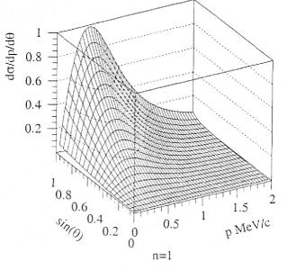
Figure 1: Spectrum of pions from ionization of $A_{2\pi}^{1S}$ atoms.

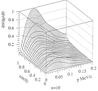
Figure 2: Spectrum of pions from ionization of $A_{2\pi}^{10S}$ atoms.

References

• [1]
• [2] R.N. Faustov, Sov. J. Particles and Nuclei, 3 (1972) 119. R. Coombles et al., Phys. Rev. Lett., 37 (1976) 249. S.H. Aronson et al., Phys. Rev. Lett., 48 (1982) 1078. J. Kapusta and A. Mocsy, “Hydrogen-like atoms from ultra relativistic nuclear collisions”, arXiv:nucl-th/9812013.
• [3] H.S.W. Massey, E.H.S. Burhop and H.G. Gilbody, Electric and Ionic Impact Phenomena, v.1, 2nd., ch.7 (Oxford Univ. Press, 1929). H.S.W. Massey and C.B.O. Mohr, Proc. R. Soc. London, A140 (1931) 605.
• [4] H.S.W. Massey and C.B.O. Mohr, Proc. R. Soc. London, A152 (1933) 613. K. Omidvar, Phys. Rev., 140 (1965) A25.
• [5] K. Omidvar, Phys. Rev., 140 (1965) A38; Phys. Rev., 188 (1969) 140 (see also refernces therein). Barut, H. Kleinert, Phys. Rev., 15 (1967) 1541. D. Trautmann, G. Baur and F. Rosel, J. Phys., B16 (1983) 3005. A.O. Barut, R. Wilson, Phys. Rev., A40 (1989) 1340.
• [6] L.L. Nemenov, Yad. Fiz., 15 (1972) 1047; Yad. Fiz., 16 (1972) 125; Yad. Fiz., 41 (1985) 980. S. Mrówczyński, Phys. Rev., D36 (1987) 1520; K.G. Denisenko and S. Mrówczyński, Phys. Rev., D36 (1987) 1529. L.G. Afanasyev and A.V. Tarasov, “Elastic form factors of hydrogenlike atoms in $nS$-states”, JINR, E4-93-293, Dubna, 1993.
• [7] B. Adeva et al., Phys. Lett. B619 (2005) 50 [First measurement of the $\pi^{+}\pi^{-}$ atom lifetime, arXiv: hep-ex/0504044]; J. Phys. G30 (2004) 1929. R. Lednicky, DIRAC note 2004-06 arXiv: nucl-th/0501065]. B. Adeva et al., Lifetime measurement of $\pi^{+}\pi^{-}$ atoms to test low energy QCD predictions (Proposal to the SPSLC, CERN/SPSLC 95–1, SPSLC/P 284, Geneva, 1995).
• [8] Proc. Int. Workshop on Hadronic Atoms “HadAtom05”, Bern, February 15-16, 2005 [L. Afanasyev, A. Lanaro and J. Schacher, arXiv:hep-ph/0508193]. Proc. Int. Workshop on Hadronic Atoms “HadAtom03”, Trento, October 13-17, 2003 [J. Gasser, A. Rusetsky and J. Schacher, arXiv:hep-ph/0401204]. Proc. Int. Workshop on Hadronic Atoms “HadAtom02”, Geneva, October 14-15, 2002 [L. Afanasyev, G. Colangelo and J. Schacher, arXiv:hep-ph/0301266].
• [9] “HadAtom99”, Proc. Int. Workshop on Hadronic Atoms, Bern, October 14-15, 1999 [J. Gasser, A. Rusetsky and J. Schacher, arXiv:hep-ph/9911339]. “Hadronic Atoms and Positronium in the Standard Model”, Proc. Int. Workshop on Hadronic Atoms, Dubna, May 26-31, 1998, Eds. M.A. Ivanov, A.B. Arbuzov, E.A. Kuraev et al. (E2-98-254, Dubna, 1998).
• [10] L. Afanasyev, A. Tarasov and O. Voskresenskaya, “Spectrum of pions from $\pi^{+}\pi^{-}$ atom breakup”, in: Proc. Int. Workshop on Hadronic Atoms “HadAtom01”, Bern, October 11-12, 2001 [J. Gasser, A. Rusetsky and J. Schacher, arXiv:hep-ph/0112293].
• [11] L.D. Landau and E.M. Lifshitz, Quantum Mechanics (Nauka Publication, Moscow, 1974).
• [12] I.S. Gradshtein and I.M. Ryzhik, Tables of Integrals, Series and Products (Nauka Publication, Moscow, 1971).
• [13] Handbook of Mathematical Functions, Eds. M. Abramowitz and I.A. Stegun (National Bureau of Standards, Applied Mathematics Series, 1964).
• [14] A. Nordsieck, Phys. Rev., 93 (1954) 785.
• [15] S. Bakmaev and O. Voskresenskaya, Part. Nucl. Lett., 3 (2006) No. 6(135) 33.
• [16] A. Sommerfeld, Ann. Phys., 11 (1931) 257.
• [17] D.A. Varshalovich, A.H. Moskalev and V.K. Khersonsky, Quantum theory of angular momentum (Nauka Publication, Moscow, 1975). A.R. Edmonds, Angular momentum in quantum mechanics (Prinston, 1957).