Predictiveness of Effective Field Theory in Nuclear Physics

Abstract

We discuss the role effective field theory plays in making predictions in nuclear physics in an approach that combines both the high sophistication of the standard nuclear many-body approach and the power of systematic higher chiral-order account in chiral perturbation theory. The main idea of this approach is illustrated with a selected number of cases involving few-body systems, the measurement of some of which poses an experimental challenge and will be of value to solar neutrino studies.

1 Introduction

Effective field theory is supposed to be an approach which can ultimately reproduce a fundamental theory and hence in principle can enable one to compute systematically corrections to approximate calculations. In nuclear physics we are supposed to have a fundamental theory, say, QCD, and so the task is to set up the scheme which comes closest to the truth encoded in QCD. There is the obvious question as to whether nuclear physics can indeed be understood in terms of QCD or put differently, how to test QCD in nuclear physics. By now this question has become akin to asking whether condensed matter systems can be understood in terms of QED. In this article, we adopt Weinberg’s “folk theorem” weinberg-folktheorem   and eschew this issue entirely.

So what is the task of an effective field theory in nuclear physics?

In addressing this question, there are two possible philosophical attitudes to take. One is to set up a well-defined effective theory within a very restricted domain of applicability, say, in energy/momentum or in the number of nucleons involved in the system and investigate whether and how the intended theory does what it is supposed to do. Here one has a well-defined set of rules for calculations and then follow $rigorously$ the rules and confirm that the strategy works. We shall call this “rigorous EFT” (RigEFT in short). In this approach, given the strong constraint imposed by the consistency with the strict chiral counting and the rapid increase of input parameters at higher orders, one is mostly limited to low orders of chiral perturbation expansion, and trying to explain the complex dynamics of wide-ranging nuclear systems is not presently feasible. In the same class of approach is what we might call “toy EFT” where an EFT with the least complexity taken into account is solved fully consistently with the set of rules adopted. The “pionless EFT” (${\pi\hskip-6.00006pt/}$EFT) to be described below belongs to this subclass. The other philosophy – which in some sense is drastically different from the ${\pi\hskip-6.00006pt/}$EFT – is, following Weinberg’s theorem, to take it for granted that EFT should work in nuclear physics and exploit the power of EFT to make calculations that cannot be accessed solely by the standard many-body technique which has been developed since many decades. This is a more physical approach aiming at describing nuclear phenomena more widely than RigEFT. We shall call this “more effective effective theory” (MEEFT) to suggest that it exploits both the power of EFT and the precision of the standard nuclear physics approach (SNPA in short).

2 SNPA and EFT

2.1 The power of SNPA

The standard approach to physics of finite nuclei and normal nuclear matter has been to determine first highly sophisticated phenomenological two-nucleon potentials implemented with multi-nucleon (typically three-nucleon) potentials fit to a large body of experimental data and solve the many-body problem as accurately as possible. This approach, on a microscopic level, has reached an impressively precise description of nuclei up to mass number $A=10$ wiringaetal with ground and excited state energies within $\sim 1$ - 2% and on a more macroscopical level, to heavy nuclei. The solution requires massive numerical computations, which some think render the approach inferior to or less elegant than analytical approaches. But in the present era of computer revolution, that is not a valid objection as it does not make the work any less fundamental than analytical calculations. This approach which we shall call “standard nuclear physics approach (SNPA)” exploits two-nucleon potentials that fit scattering data up to momenta $\sim 300$ MeV with a $\chi^{2}$/datum $\mathrel{\hbox to0.0pt{\lower 3.0pt\hbox{\hskip 1.0pt$\sim$}\hss}\raise 1.0pt\hbox{$<$}}1.4$. The success of this approach has been extensively reviewed in SNPA1 ; SNPA and we will not elaborate any further on the SNPA per se, although we will refer to it throughout this chapter. It should be stressed that it would be a grave mistake to ignore the accuracy achieved by the SNPA and discard it as is done in some circle of workers in the field on the ground that it is not derived in EFT formalism. Our point of view which we will develop here is that we should – and can – incorporate it in the framework of an EFT in such as way as to allow us to systematically control possible corrections brought in by more fundamental and systematic formulation.

2.2 The power of EFT

In assessing both the power and the limitation of the SNPA, the physical observables to look at are not only the spectra of the states involved but also response functions involving wave functions and currents. For the latter, the standard procedure that has been mostly employed is to write down the currents in terms of the single-particle operators – called impulse approximation – which are typically the most important and then make, often less important, corrections due to the presence of multi-body operators constructed from the exchange of mesons, called “meson-exchange currents,” in an effective phenomenological Lagrangian field theory. This approach was first systematized in CR71 . In many of the applications, this approach gives results that compare well with experiments. But within the framework of many-body theory based on phenomenological potentials, however, there is no unique or systematic way to assess what the size of corrections is, so when the calculated value disagrees with experiments, there is no well-defined and systematic way to improve the calculation. One is thus allowed to make post-dictions but rarely predictions or calculations that are free of free parameters. This is one place where EFT can come in to help.

What is the true use of an EFT? To show that QCD works is not the objective as mentioned above in accordance with Weinberg’s folk theorem. In essence QCD should work in nuclei if one works hard enough. This we are witnessing in the construction of two-body potentials in $\chi$PT.  What have been done in the literature in the past in addressing the issue in question are the following:

• One direction belonging to the RigEFT class followed by a large number of workers in the field is to limit oneself to a well-defined, but drastically simplified, EFT Lagrangian and then study this as rigorously as possible within the framework of suitably well-defined rules. A case that has been widely studied is the so-called “pionless (${\pi\hskip-6.00006pt/}$)” Lagrangian approach in which $all$ but nucleon fields are integrated out (e.g., pionless-chenetal and for a review, see bedaque-vankolck ). Covering by fiat a limited range of nuclear interactions, it is necessarily limited in scope and so far achieved no more than $reproducing$ what is already well and accurately described in SNPA. While this approach has the advantage to directly address problems that can lead to exact statements, such as the phenomenon of renormalization-group limit cycle, Efimov effect etc. (see, e.g., hammer ), it lacks predictiveness that one would hope for.

  An approach that belongs to the RigEFT class but comes closer in principle to the MEEFT class takes the nucleon and the pion as the relevant degrees of freedom and calculate to as high an order as feasible and as consistently as possible within the tenet of chiral perturbation theory. This calculation is limited in that the number of unknown constants increases rapidly as the chiral order increases. We will not have much to say on this approach in this article. But when we say RigEFT without specification, we will mean both this and the pionless EFT.

• The other direction which we shall adopt in this paper as explained in detail elsewhere MR-taiwan is to exploit the strategy of an EFT to calculate quantities that neither the SNPA nor QCD proper separately can do, that is, to make “predictions.” By predictions, here, we mean parameter-free calculations with error estimates of what might be left out in the approximations, e.g., the truncation, involved. The strategy is to exploit both the full machinery of SNPA $and$ the power of EFT in a scheme that is consistent with the symmetries of QCD in the spirit of Weinberg’s theorem to make $predictions$ that can be confronted with Nature. We will tacitly assume that systematic high-order chiral perturbation calculations of the potentials will eventually provide quantitative support to the potentials used in the SNPA. Up to date, this assumption is justified as summarized in  machleidt06 .

3 Chiral Lagrangians

3.1 Relevant Scales and Degrees of Freedom

When applied to nuclear systems, an EFT involves a hierarchy of scales in the interactions. In nuclear physics, the nucleon is the core degree of freedom defining the system with the pion figuring as the lightest mesonic degree of freedom. What other degrees of freedom must enter in the dynamics depends upon what problem one is looking at. If the kinematics probed is of the scale $E\ll m_{V}$ where $m_{V}$ is the mass of the light-quark vector mesons, the lightest of which are the $\rho$ and the $\omega$, then one may “integrate out” all the vector mesons and work with the baryon and the pion only. This regime is accessible by a chiral perturbation theory ($\chi$PT) for physics of dilute nuclear systems, e.g., few-nucleon systems. If one works to high enough order in chiral perturbation theory, one can hope to understand much of nuclear physics taking place within the given restricted kinematic domain, although in some cases, it is more convenient and simpler to introduce heavier degrees of freedom explicitly as for instance the $\rho$, $\omega$, $a_{1}$, $\sigma$ etc. When one is studying systems involving a scale $E\ll m_{\pi}$, where $m_{\pi}$ is the pion mass, then one might even “integrate out” the pion as well, as is done in ${\pi\hskip-6.00006pt/}$EFT. How this program works is described in numerous lecture notes, one nice reference of which is kaplan-berkeley .

It should be remarked that even when ${\pi\hskip-6.00006pt/}$ EFT is fully justified, that is, pions are $not$ indispensable, in certain cases, it proves to be much more powerful and predictive to keep pions as effective degrees of freedom. We will encounter such a situation when we discuss the so-called “chiral filter mechanism.” One finds that having explicit pion degrees of freedom with their associated low-energy theorems can give a highly simplified and efficient description of a process which would require much harder work if the pion were integrated out.

More significantly, the explicit presence of pions is now known to be the dominant element in describing the structure of light nuclei. In particular, to quote Wiringa wiringa06 , “the success of the simple model [of light nuclei] supports the idea that the one-pion exchange is the dominant force controlling the structure of light nuclei …”

As one probes denser systems such as nuclear matter and denser matter, due to BR scaling (recently reviewed BHLR06 ), the vector meson mass drops and near chiral restoration, becomes comparable to the pion mass. In this case, one cannot integrate out the vector mesons; the vector fields have to be endowed with local gauge invariance, so that systematic chiral perturbation can be done with the vector mesons included HY:PR .

3.2 Vector mesons and baryons

It has been recently discussed as to how hidden local symmetry emerges if one wants to “obtain” an effective field theory from a fundamental theory. Interestingly, a hidden local symmetry (HLS) involving an infinite tower of gauge fields coupled to pions in a chirally symmetric way emerges from string theory via holographic duality. One refers to such a theory “holographic dual QCD.” Now one can view the hidden local symmetry approach of Harada and Yamawaki HY:PR with the light-quark vector mesons as a truncated version of the holographic dual QCD. Restricted to the lowest members of the vector mesons, i.e., the $\rho$ and $\omega$, it is the Wilsonian matching to QCD that makes the theory a bona-fide effective theory of QCD. In the simplest form of HLS theory with $N_{f}=3$, there are the octet pseudo-Goldstone bosons and nonet of vector mesons coupled gauge invariantly. Baryon fields do not figure explicitly. However holographic dual QCD suggests that baryons must appear as skyrmions. Although there have been efforts to construct skyrmions with a chiral Lagrangian with vector mesons incorporated (see weigel-IJMP for references) – and it is now clear that vector mesons must be present in the skyrmion structure, very little is understood of such hidden local symmetry skyrmions. For the purpose of this section, instead of generating baryons as solitons, we will simply introduce baryon fields explicitly.

3.3 Baryon fields

Baryon fields are to be treated as “matter” fields, which is fine as long as the momentum transfer involved is $\ll\Lambda$ where $\Lambda$ is the cutoff. We generally consider baryons made up of $u$, $d$ and $s$ quarks, i.e., $SU(3)_{F}$ although we will be concerned only with two flavors in this article . We want the baryon field $B$ to be invariant under (vector flavor) $SU(3)_{V}$,

$$B\rightarrow VBV^{\dagger}$$ (3.1)

with $V\in SU(3)_{L+R=V}$. Now how does $B$ transform under $SU(3)_{L}\times SU(3)_{R}$? Here there is no unique way as long as it is consistent with the symmetries of QCD. For our purpose, the most convenient choice is to have it transform as

$$B\rightarrow hBh^{\dagger}$$ (3.2)

with

$$\xi_{L} \rightarrow h\xi_{L}L^{\dagger},$$ (3.3)

$$\xi_{R} \rightarrow h\xi_{R}R^{\dagger}$$ (3.4)

where

$$U=\xi_{L}^{\dagger}\xi_{R}.$$ (3.5)

Here $h$ is a complicated local function of $L\in SU(3)_{L}$, $R\in SU(3)_{R}$ and $U\in SU(3)_{V}$, the explicit form of which is not needed. When $L=R=V$, it is just a constant $h=V$.

We define in unitary gauge $\xi_{L}^{\dagger}=\xi_{R}=e^{i\pi/F_{\pi}}$

$$A_{\mu} = \frac{i}{2}\left(\xi^{\dagger}\partial_{\mu}\xi-\xi\partial_{\mu}\xi^{\dagger}\right),$$ (3.6)

$$V_{\mu} = \frac{1}{2}\left(\xi^{\dagger}\partial_{\mu}\xi+\xi\partial_{\mu}\xi^{\dagger}\right),$$ (3.7)

$$D_{\mu}B = \partial_{\mu}+[V_{\mu},B]$$ (3.8)

transforming under $SU(3)\times SU(3)$ as

$$A_{\mu} \rightarrow hA_{\mu}h^{\dagger},$$ (3.9)

$$V_{\mu} \rightarrow h(\partial_{\mu}+V_{\mu})h^{\dagger}.$$ (3.10)

Now what we need to do is to write the Lagrangian ${\cal L}_{inv}$ invariant and the Lagrangian ${\cal L}_{non}$ non-invariant under the given transformation. Thus

$${\cal L}_{inv} = {\rm Tr}\bar{B}(i\gamma^{\mu}D_{\mu}-m_{0})B-D{\rm Tr}\bar{B}\gamma^{\mu}\gamma_{5}\{A_{\mu},B\}$$ (3.11)

$$-F{\rm Tr}\bar{B}\gamma^{\mu}\gamma_{5}[A_{\mu},B]+\cdots,$$

$${\cal L}_{non} = a_{1}{\rm Tr}\bar{B}(\xi^{\dagger}M\xi^{\dagger}+{\rm h.c})B+a_{2}{\rm Tr}\bar{B}B(\xi^{\dagger}M\xi^{\dagger}+{\rm h.c.})$$ (3.12)

$$+a_{3}{\rm Tr}(MU+{\rm h.c.}){\rm Tr}\bar{B}B+\cdots$$

Here the ellipses stand for higher order terms, either in derivatives or in quark mass terms or in combination of both. $m_{0}$ is the dynamically generated mass of the baryon which is of order $\sim 1$ GeV, i.e., the chiral scale.

In nuclear physics at low energy we are considering, the nucleon is non-relativistic, so it makes sense to go to the non-relativistic form of the Lagrangian. In fact for the development of the principal thesis of this article, it is preferable. A nice way of going to the non-relativistic form is the heavy-baryon formalism heavybaryon . To do this, define

$$B_{v}(x)=e^{im_{0}v\cdot\gamma v\cdot x}B(x)$$ (3.13)

and introduce the spin operator $S_{v}^{\mu}$ that satisfies

$$v_{\mu}S_{v}^{\mu}=0,\ S_{v}^{2}B_{v}=-\frac{3}{4}B_{\nu},$$ (3.14)

and

$$\{S_{v}^{\mu},S_{V}^{\mu}\}=\frac{1}{2}(v^{\mu}v^{\nu}-\eta^{\mu\nu}),$$ (3.15)

$$[S_{v}^{\mu},S_{V}^{\nu}]=i\epsilon^{\mu\nu\alpha\beta}v_{\alpha}S_{v\beta}.$$ (3.16)

In terms of these definitions, we can rewrite ${\cal L}_{inv}$ as

$${\cal L}_{inv}= {\rm Tr}\bar{B}_{v}v_{\mu}D^{\mu}B_{v}+2D{\rm Tr}\bar{B}_{v}S_{v}^{\mu}\{A_{\mu},B_{v}\}$$ (3.17)

$$+2F{\rm Tr}\bar{B}_{v}S_{v}^{\mu}[A_{\mu},B_{v}]+\cdots$$

In this form the mass term $m_{0}$ disappears, so the chiral counting comes out as we wanted without having to worry about the cancelation between the mass term and the time derivative on the baryon field. Similar forms can be written down for the chiral symmetry non-invariant terms.

The Lagrangians written above in bilinears in the baryon field are applicable in the one-nucleon sector. With these Lagrangians in various approximations, one can systematically treat one baryon problem including interactions with pions and external fields. If one is interested in this topic, there are some good reviews in the literature which show that chiral perturbation theory does work well and could even be improved as one goes to higher orders and as more precise experimental data become available. In what follows and in other sections of this paper, we will take this “success” for granted.

Here we are interested in few- as well as many-nucleon systems. When there are more than one nucleon in the system, one has multi-nucleon terms involving $2n$ Fermion fields for $n>2$. Thus we have

$${\cal L}_{2n-fermi}=\sum_{a}(\bar{B}\Gamma_{a\mu}B)(\bar{B}\Gamma_{a}^{\prime\mu}B)+\cdots$$ (3.18)

where the ellipses now stand for higher number of Fermi fields and $\Gamma$ and $\Gamma^{\prime}$ are various Lorentz structures involving derivatives etc. subject to the necessary symmetry constraints of QCD.

If one wishes, the light-quark vector mesons can be incorporated in a hidden-gauge symmetric way although there are certain ambiguities which are not present in the skyrmion approach mentioned above. In this article, we won’t need vector degrees of freedom since their masses are of higher scale than the appropriate cutoff in the density regime we are considering.

4 Pionless EFT

As mentioned, if one is interested in nuclear processes where the energy scale is much less than the pion mass, one may integrate out the pion as well. The resulting Lagrangian containing only the massive nucleons has no chiral symmetry since there are no pions anymore. But chiral symmetry is not violated. It is just that chiral symmetry is an irrelevant symmetry here. It is easy to write down the effective Lagrangian

$${\cal L}_{\not\pi} = N^{\dagger}(i\partial_{t}+\nabla^{2}/2m)N$$ (4.19)

$$+C(N^{\dagger}N)^{2}+C^{\prime}((NN)^{\dagger}(N\nabla^{2}N)+\cdots$$

where $N$ stands for the nucleon doublet replacing the baryon field $B$. The ellipsis stands for terms with spin and flavor matrices and other derivative terms of the same order with and without spin and isospin factors etc. The Lagrangian should be Galilean invariant.

Given the extreme simplicity of the pionless Lagrangian, the power counting rule is equally simple allowing one to do a systematic and consistent calculation in principle to high orders. It is just a power series in $p/\Lambda$ where $p$ is the probe momentum and $\Lambda$ is the cutoff scale defining the momentum space considered. In practice it makes no sense to go to very high orders since unknown parameters increase rapidly. Further complications can arise if one is interested in many-nucleon systems where the Fermi momentum which is of order of a few times the pion mass enters but this theory makes no sense there anyway.

Now what can we learn with this? As already mentioned, actually little more than that an EFT works for effective range theory. It can work for two-body and perhaps three-body systems for which the SNPA has scored a great success already but the procedure gets rapidly unmanageable when it goes to the really interesting problem like the solar $hep$ and the related $hen$ process that involve four-body interactions. (We will return to this problem below.) It has no pions and hence quantities which are rendered easy to understand when pions are present (various low-energy theorems ..) are made difficult, if not impossible (as we will see later). Being a toy model, it allows systemization and completeness in describing certain but restricted low-energy processes thanks to the simplicity of the Lagrangian. But it should be mentioned that the physical processes that can be treated are mostly, if not all, those which have been well reproduced since ages in SNPA with well-defined corrections (e.g., those processes which are subsumed in effective range theory).

As an illustration, consider $n+p\rightarrow d+\gamma$ at low energy which has been heralded as a success of the model kaplan-berkeley and to which we will return below for MEEFT. The $np$ capture at thermal energy is accurately measured, and so can offer an excellent process to check the theory with. Now this process is dominated by an isovector $M1$ operator, so in (4.19), we need the interaction $C$ term for the ${}^{3}S_{1}$ channel, a $C^{\prime}$ term for both ${}^{3}S_{1}$ and ${}^{1}S_{0}$ channels and the couplings to the magnetic photon

$${\cal L}^{1b}_{B}=eN^{\dagger}(\kappa_{S}+\kappa_{V}\tau_{3})\frac{{\mathbf{\sigma}}\cdot{\mathbf{B}}}{2m}N$$ (4.20)

and

$${\cal L}^{2b}_{B}=eL_{1}(N^{T}P_{i}N)^{\dagger}(N^{T}{\overline{P}_{3}}N)B_{i}$$ (4.21)

where $\kappa_{S/V}=\frac{1}{2}(\kappa_{p}\pm\kappa_{n})$ with $\kappa_{p}=2.79$ and $\kappa_{n}=-1.91$. Here $P_{i}$ and $\overline{P}_{3}$ are, respectively, the ${}^{3}S_{1}$ and ${}^{1}S_{0}$ projection operators. The constant $C$ in (4.19) is obtained by fitting the deuteron binding energy and the $C^{\prime}$ from the effective range in $NN$ scattering. But there is one unknown constant $L_{1}$ which cannot be a priori fixed: There is no other experiment than the $np$ capture that involves this term and hence no true prediction can be made. It is not however totally devoid of value since once $L_{1}$ is fixed from the $np$ capture experiment, one can then turn the process around and calculate the inverse process $\gamma d\rightarrow n+p$ as a function of the photon energy. It works fairly well up to, say, $E_{\gamma}\sim 10$ MeV. This is relevant for big-bang nucleosynthesis  kaplan-berkeley . One should however recognize that there is no real gain in theoretical understanding in this approach because the SNPA can do just as well with well-defined two-body corrections.

5 MEEFT

5.1 Weinberg’s counting rule

We now turn to a more predictive EFT scheme. To exploit the accuracy and power of SNPA, we adopt the Weinberg counting rule. In fact the Weinberg countingweinberg-counting1 ; weinberg-counting2 is the only way that the SNPA can be “married” with an EFT. Since the aim here is to exploit the powers of both SNPA and EFT, we refer to this as “MEEFT (more effective effective field theory).”

The Weinberg counting consists essentially of two steps. In the first step, one defines the nuclear potential as the sum of 2-particle irreducible diagrams – irreducible in the sense that they contain no purely nucleonic intermediate states – and truncates the sum at some order $n$ in the standard chiral perturbation power counting. The potential is dominated by two-body irreducible terms with $n$-body terms with $n>2$ terms suppressed by the power counting. In the second step, the potential so constructed is used to solve the Lippman-Schwinger or Schrödinger equations. This corresponds to incorporating “reducible” graphs that account for infrared enhancement (or singularities) associated with bound states etc. Now the potential will then include one or more pion exchanges and local multi-fermion interactions that represent massive degrees of freedom (such as the vector mesons $\rho$, $\omega$ etc.) that are “integrated out.” The approach can then be applied not only to few-nucleon processes but also to many-nucleon processes with the outputs in the form of physical observables, namely, scattering cross sections, energy spectra, response functions to external fields etc. Wave functions make an indispensable part of the scheme, so the theory enables one to calculate things not only in few-body systems but also across the periodic table. Contact with “rigorous” EFT – in the sense of power counting assured, e.g., in pionless EFT – can be made only for few-body systems. However systematic higher order chiral corrections to the estimates made in SNPA can be made with certain error estimates for processes that involve heavy nuclei, e.g., lead nuclei. This feat has not been feasible up to date in the ${\pi\hskip-6.00006pt/}$EFT approach

The Weinberg counting rule explains automatically that n-body forces with $n>2$ are suppressed relative to 2-body forces and n-body currents are normally subdominant to one-body current, known in nuclear physics as impulse approximation etc. These are familiar things in SNPA but in MEEFT, they go beyond SNPA in that one can in practice make a systematic account for corrections to the SNPA results that are guided by an effective field theory strategy. What this means is that in calculating response functions to external fields, one can use the accurate state-of-the art wave functions that have been constructed since a long time in SNPA to make “predictions” that are otherwise not feasible in the RigEFT approach. We will illustrate this point below.

There is of course a price to pay for this “predictive power.” One of them is possible ambiguity in the regularization procedure which separates high-energy and low-energy physics. Where to do the separation is completely arbitrary and the observables calculated should not depend on the separation point. This is the statement of the renormalization group invariance. However to the extent that one calculates in certain approximation, one cannot make the independence perfect. As it stands at present, how best to do this can be more an art than science.

Figure 1: A two-loop diagram that requires higher-order counter term in the leading order graph in ${\pi\hskip-6.00006pt/}$EFT.

To cite a specific case, one of the (counting) problems arises when the two-loop graph with a pion exchange between two nucleons of Fig. 1 treated as a Feynman diagram is calculated in dimensional regularization. The problem lies in treating this graph strictly in the sense of perturbation theory. We will see later that this is $not$ what is done in MEEFT. If one writes the dimension as $d=4-2\epsilon$ where we want $\epsilon\rightarrow 0$, then one finds that this graph diverges as

$$\sim\frac{1}{\epsilon}m_{\pi}^{2}.$$ (5.22)

This represents the logarithmic dependence on scale $\sim\ln\mu$. This scale dependence needs to be canceled by a counter term that goes like $\sim m_{\pi}^{2}$. In the power counting of the theory, this comes at higher order than that assigned to the pion exchange in Weinberg counting since $m_{\pi}^{2}$ counts as ${\cal O}(Q^{2})$. This means that when one solves Schrödinger equation with the pion exchange included in the potential consisting of irreducible terms, one has an inconsistency in chiral counting since the pion exchange needs to be regulated by a counter term higher order in the Weinberg counting.

Now how did this “basic” problem not hamper development in SNPA? The answer is that what happens in nuclei is not wholly accessed by perturbative renormalization that is obstructed by the above problem. The fact that one is solving Schrödinger equation illustrates that nuclear problems are inherently non-perturbative and the above inconsistency arises because one is doing a perturbation calculation. This difficulty is essentially sidestepped by MEEFT that we will discuss in the following section.

There is also a possibility that this regularization difficulty can even be $formally$ remedied vankolcketal1 ; arriola1 . One of the most serious is the singularity of tensor interactions in partial waves where the interaction is attractive. For large cutoff $\Lambda$, say, greater than vector meson mass, spurious bound states can be generated. Of course the cutoff has a physical meaning in effective theories as elaborated further below and picking a cutoff bigger than what is appropriate is meaningless, so this problem is in a sense academic. However even for low enough cutoff, there may be unacceptably large cut-off dependence. The situation gets more serious in certain channels where counter terms are infrared-enhanced. However it turns out that one can add a counter term in each partial wave where this sensitivity is present and avoid this difficulty, at least to the leading ordervankolcketal1 . It is not clear that this problem continues to arise at higher orders and more work is needed in this area. This issue is revisited in epelbaum-meissner06 . At present, the MEEFT predictions described below are free from this difficulty.

5.2 Strategy of MEEFT

What is crucial for a viable MEEFT is to have very accurate wave functions. Let us suppose that we do have wave functions that give a good description of spectra and response functions for a range of mass numbers. The basic requirement is that the wave functions so obtained possess the correct long-distance properties governed by chiral symmetry. We shall assume that the wave functions we use meet this requirement. It would be highly surprising if fitting a large number of low-energy data, both scattering and current matrix elements, can be achieved without a good account of the long-distance physics associated with chiral symmetry. We can therefore assume that the currents we construct in Weinberg’s scheme incorporating one or more pion exchanges given by leading order chiral expansion should be consistent with the (SNPA) wave functions up to that order, with uncertainty in the current residing in higher order. Shorter-distance properties of the range $\mathrel{\hbox to0.0pt{\lower 3.0pt\hbox{\hskip 1.0pt$\sim$}\hss}\raise 1.0pt\hbox{$>$}}(2m_{\pi})^{-1}$ in the phenomenological potentials used to generate the wave functions are not unique, but they should not affect long wavelength probes we are interested in. If we can assure cutoff independence within a range consistent with the physics we are looking at, that should be good enough for a genuine prediction. One could use renormalization group arguments to support this statement. Now the strategy in computing response functions is to calculate the irreducible contributions to the current vertex functions to the order that is correctly implemented in the wave functions from the point of view of chiral counting. In doing this, we can roughly separate into two classes of processes: those processes that are chiral-filter protected and those that are not. The former processes are accurately calculable given accurate wave functions with small error bars since the effects are primarily controlled by soft-pion theorems. The latter is less well controlled by low-energy theorems and hence brings in certain uncertainties. We will show however that with an astute implementation of SNPA, one can calculate certain processes belonging to the second class with some accuracy. We will treat both classes below.

5.3 The “chiral filter”

We will be dealing with a slowly varying weak external field, with the external field acting only once at most. This means that in the chiral counting, the external field that does not bring in small parameters such as the external momentum or the pion mass lowers by one chiral order two-body corrections relative to the single-particle process to the counting that goes into the potential. This is essentially because of the minimal coupling of the external field which replaces one derivative in the two-body terms by the external field that contribute to the potential. This means that if we know the potential to $n$-th chiral order, then there can be a two-body current which, when not suppressed by symmetry, is determined to the same order, further corrections being suppressed by two chiral orders. This makes the calculation of the correction terms extremely accurate. This does not take place if the external field brings into the current operators extra small parameters such as the external momentum or the pion mass. It is known that this chiral filter is operative with the isovector $M1$ and the axial-charge operators in nucleiKDR ; MR91 , but not with the isoscalar $M1$ and the Gamow-Teller operators as we will see later.

The idea of chiral filter explained more precisely below was a guiding principle when EFT formalism was not available for nuclear physics. In chiral perturbation theory, chiral filter is automatic, so there appears to be no big deal in it when one does a systematic chiral expansion to high enough order but the intuitive power associated with pion dynamics is completely lost when the pion is integrated out as in the pionless EFT. An illustrative example is the thermal $np$ capture which can be predicted without any parameters in MEEFT but can only be postdicted with one unknown parameter in the pionless theory. The point is that even if it were possible to do a systematic chiral counting in ${\pi\hskip-6.00006pt/}$EFT and obtain certain results perhaps painlessly, the simplicity brought in by chiral symmetry would be lost.

5.4 Working of MEEFT

In order to illustrate how MEEFT supplemented by the chiral filter mechanism works out in nature, let us study the response functions in the mass number $A$ system where we have at our disposal accurate wave functions for $A-1$, $A$ and $A+1$ systems. We shall do so with few-nucleon systems. For heavy nuclei and nuclear matter, we cannot proceed in the same approach and hope to obtain accuracy. For that purpose, we need to develop the notion of “double decimation” as we shall mention in the last section.

We want to treat specifically $A=2,3,4$ systems on the same footing. The processes we are interested in are

$$n+p \rightarrow d+\gamma,$$

$$p+p \rightarrow d+e^{+}+{\nu}_{e},$$

$$\nu_{e}+d \rightarrow e^{-}+p+p,$$

$$e+d \rightarrow e+d,$$

$$p+^{3}{\rm He} \rightarrow {}^{4}{\rm He}+e^{+}+\nu_{e},$$

$$n+^{3}{\rm He} \rightarrow {}^{4}{\rm He}+\gamma.$$ (5.23)

These are processes that are of interest not only for nuclear physics but also for astrophysical studies. The first four processes were postdicted in the ${\pi\hskip-6.00006pt/}$EFT with undetermined parameterschen-np-supp ; ravndal-pp and the last two cannot be accessed even for postdiction. The third process is one of the class of reactions for SNO processes studied in EFT andoetal-neutrino , involving both the charge current (CC) processes

$$\nu_{e}+d \rightarrow e^{-}+p+p,$$

$$\bar{\nu}_{e}+d \rightarrow e^{+}+n+n$$ (5.24)

and the neutral current (NC) processes

$${\nu}_{l}+d \rightarrow {\nu}_{l}+p+n,$$

$$\bar{\nu}_{l}+d \rightarrow \bar{\nu}_{l}+p+n.$$ (5.25)

Here $l={\mbox{e}},\mu,\tau$. These neutrino processes are very closely related to the $pp$ process as they are governed by the same operators, albeit at different kinematics. They can be $predicted$ with an accuracy comparable to that of the $pp$ process andoetal-neutrino . The fourth process, electron-deuteron scattering, can be treated in various versions of EFT with some accuracy for momentum transfer $Q^{2}<1$ GeV². All the processes in (5.23) have been treated in SNPA but for reasons not difficult to pin-point, various calculations gave different results ranging in some cases over several orders of magnitude. The problem there was that there was no systematic way of estimating errors involved and making corrections. We will see how the chiral filter works in enabling one to make an accurate (parameter-free) prediction for the isovector transition in the $np$ capture and how it provides a way to compute the processes that are not protected by the chiral filter. The last of (5.23)– the $hen$ process – has not yet been fully calculated in the approach described in this paper. However the current is completely determined with the formalism described here and there is nothing to prevent a totally parameter-free calculation as we shall argue.

5.4.1 What can the chiral filter say?

Historically it was the special role played by the pion that led to an early and simple understanding riska-brown of the thermal $np$ capture process in (5.23). Now we know that the chiral filter mechanism is automatically included in a systematic chiral expansion in MEEFT, so there is no big deal in it from the point of view of chiral symmetry but the power of it is in highlighting where and in which way pions can play a prominent role in certain processes, without requiring to go to higher orders in chiral expansion and in avoiding unknown parameters. It has the power to presage what one can or cannot do with calculable leading corrections. This was first noticed in the application of current algebras, i.e., soft-pion theorems, to the nuclear processes of the type given in (5.23)KDR and subsequently justified in $\chi$PT MR91 . The argument went as follows.

In MEEFT, effective currents are characterized by the number of nucleons involved in the transition. The leading one (in the chiral counting) is the single-particle opeerator (called one-body or impulse), then the next subleading one is two-particle (two-body) followed by three-particle etc. The Weinberg counting says that in the processes we are concerned with, we can limit ourselves to up to two-body. It has indeed been verified that three-body and higher-body corrections can be safely ignored. Now among two-body currents, the leading correction will be given by the one-pion exchange as depicted in Fig.2.

Figure 2: Two-body currents with one soft-pion exchange which dominate whenever unsuppressed by kinematics or symmetry. The cross stands for the current. Both (a) and (b) contribute to the vector current but only (a) contributes to the axial current.

This is the longest-range correction. Shorter-ranged corrections involve higher derivative terms, pion loop diagrams and corresponding counter terms. If the one-pion exchange contribution can contribute unsuppressed by kinematics or symmetries, then we have a chance to estimate the leading corrections with confidence free of parameters. Since the $\pi NN$ vertex is known, what matters then will be the vertex $J_{\mu}\pi NN$ where $J_{\mu}=V_{\mu}^{a},\ A_{\mu}^{a}$ with the index $a$ standing for the isospin (flavor). Now the longest wavelength process that enters here will be the graph with the pion being “soft.” When the pion is soft, there is a low-energy theorem that gives for the vector current

$$\sim {\cal O}(\frac{p}{m_{N}})\ \ \ \ \ \ {\rm for}\ \ \ \mu=0,$$ (5.26)

$$\sim \frac{g_{A}}{F_{\pi}}\epsilon^{3ab}\frac{\tau^{a}}{2}{\mathbf{\sigma}}\ \ {\rm for}\ \ \ \mu=1,2,3$$ (5.27)

and for the axial vector current

$$\sim \frac{1}{F_{\pi}}\epsilon^{abc}V_{0}^{c}\ \ {\rm for}\ \ \ \mu=0,$$ (5.28)

$$\sim {\cal O}(\frac{p}{m_{N}})\ \ \ \ \ \ {\rm for}\ \ \ \mu=1,2,3.$$ (5.29)

Here $m_{N}\sim 1$ GeV is the lowest baryon, i.e., nucleon mass. The characteristic momentum scale involved, say, momentum carried by the nucleon responding to the external field, is assumed to be much smaller than the baryon mass scale. What these results imply is quite simple. They say that the two-body corrections are dominated by the soft-pion exchanges in the space component of the vector current, e.g., the isovector $M1$ transition and in the time component of the axial vector current, e.g., the first forbidden beta transitions $J^{\pm}\rightarrow J^{\mp}$ with $\Delta T=1$. As a corollary, we learn that the two-body currents for the time component of the vector current, e.g., the charge operator and the space component of the axial current, e.g., the Gamow-Teller transition have no reason to be unsuppressed. In contrast, the leading order one-body current has the opposite behavior, namely, the space component of the one-body vector current and the time component of the one-body axial current are suppressed relative to the other components. Table 1 illustrates what sorts of chiral orders are involved for the vector current in this way of counting. A similar scaling applies to the axial current.

	$V^{i}$	$V^{0}$
one-body current	${\cal O}(Q^{1})$	${\cal O}(Q^{0})$
two-body (leading)current	${\cal O}(Q^{2})$	${\cal O}(Q^{3})$
two-body (one loop)current	${\cal O}(Q^{4})$	${\cal O}(Q^{4})$
$M_{2b}$/$M_{1b}$	${\cal O}(Q^{1})$	${\cal O}(Q^{3})$

Table 1: Various contributions to the vector current relative to the one-body charge $V^{0}\sim{\cal O}(1)$.

5.4.2 Sketch of the calculational procedure

While the calculation involves a conceptually simple procedure, the details are rather complicated. We shall therefore skip the details and instead present a brief sketch of the calculational procedure focusing more on the essential concepts.

In the Weinberg counting scheme, the relevant quantity is the index $\nu$ in the chiral counting of the electroweak currents. In the present case it is sufficient to focus on “irreducible graphs” in Weinberg’s classification. Irreducible graphs are organized according to the chiral index $\nu$ given by

$$\nu=2(A-C)+2L+\sum_{i}\nu_{i}\,,$$ (5.30)

where $A$ is the number of nucleons involved in the process, $C$ the number of disconnected parts, and $L$ the number of loops; $\nu_{i}$ is the chiral index $\nu\equiv d+e+\frac{n}{2}-2$ of the $i$-th vertex where $d_{i}$ is the number of derivatives, $e$ the number of the external field ($=1$) and $n_{i}$ the number of internal nucleon lines, all entering the $i$-th vertex. One can show that a diagram characterized by eq.(5.30) involves an $n_{B}$-body transition operator, where $n_{B}\equiv A-C+1$. The physical amplitude is expanded with respect to $\nu$. The leading-order one-body GT operator belongs to $\nu$=0. Compared with this operator, a Feynman diagram with a chiral index $\nu$ is suppressed by a factor of $(\breve{q}/\Lambda_{\chi})^{\nu}$, where $\breve{q}$ is a typical three-momentum scale or the pion mass, and $\Lambda_{\chi}\sim$ 1 GeV is the chiral scale. We denote this in short as $Q^{\nu}$. In our case it is important to take into account also the kinematic suppression of the time component of the nucleon four-momentum. We note

$$v\cdot p_{l}\sim v\cdot p_{l}^{\prime}\sim v\cdot k_{l}\sim\frac{\breve{q}^{2}}{m_{N}},$$ (5.31)

where $p_{l}^{\mu}$ ($p_{l}^{\prime\mu}$) denotes the initial (final) momentum of the $l$-th nucleon, and $k_{l}^{\mu}\equiv(p_{l}^{\prime}-p_{l})^{\mu}$. Therefore, each appearance of $v\cdot p_{l}$, $v\cdot p_{l}^{\prime}$ or $v\cdot k_{l}$ carries two powers of $\breve{q}$ instead of one, which implies that $\nu$ increases by two units rather than one. Thus, if we denote by $q^{\mu}=(q_{0},\mathbf{q})$ the momentum transferred to the leptonic pair, say, in the $pp$ and $hep$ processes in eqs.(5.23), then $q_{0}\sim|\mathbf{q}|$$\sim q^{2}/\Lambda_{\chi}$ $\sim{\cal O}(Q^{2})$ rather than ${\cal O}(Q)$ as naive counting would suggest. These features turn out to simplify the calculation considerably.

In what follows, unless otherwise stated, we will always count correction terms relative to the leading-order terms. Since the leading-order terms in the currents are of ${\cal O}(Q^{0})$, a chiral order corresponding to the index $\nu$ will often be referred to as N^νLO; $\nu$=1 corresponds to NLO (next-to-leading order), $\nu$=2 to N²LO (next-to-next-to-leading order), and so on. In this discussion, we shall limit ourselves to N³LO. One can go to N⁴LO for certain operators as was done in the published calculation hep but this is not needed for our purpose here.

We now briefly sketch the structure of one-body (1B) and two-body (2B) current operators that are consistent with the chiral counting. Of course actual calculations have to go into the nitty-gritty details.

The current in momentum space is written as

$$J^{\mu}({\mathbf{q}})=V^{\mu}({\mathbf{q}})+A^{\mu}({\mathbf{q}})=\int\!d{\vec{x}}\,{\mbox{e}}^{-i{\mathbf{q}}\cdot{\vec{x}}}J^{\mu}({\vec{x}}).$$ (5.32)

We shall use the obvious notations $V^{\mu}=(V^{0},\,{\mathbf{V}})\,,\;\;\;\;A^{\mu}=(A^{0},\,{\mathbf{A}})$.

The chiral counting of the electroweak currents is summarized in Table 2, where the non-vanishing contributions at ${\mathbf{q}}=0$ are indicated. This table shows how the counting goes for each component of the currents:

• $\nu$ = 0 : One-body ${\mathbf{A}}$ and $V^{0}$: ${\mathbf{A}}$ gives the Gamow-Teller (GT) operator, while $V^{0}$ is responsible for the charge operator.

• $\nu$ = 1 : One-body $A^{0}$ and ${\mathbf{V}}$: $A^{0}$ gives the axial-charge operator while ${\mathbf{V}}$ gives the M1 operator.

• $\nu$ = 2 : Two-body tree current with $\nu_{i}=0$ vertices, namely, the soft-pion-exchange current. This is the leading correction protected by chiral filter to the one-body M1 and axial-charge operators carrying an odd orbital angular momentum.

• $\nu$ = 3 : Two-body tree currents with $\sum_{i}\nu_{i}=1$. These are leading corrections to the GT and $V^{0}$ operators carrying an even orbital angular momentum. These are chiral-filter $unprotected$ and hence involve constants that are not given by chiral symmetry considerations (e.g., soft-pion theorems) alone.

• $\nu$ = 4 : All the components of the electroweak current receive contributions of this order. They consist of two-body one-loop corrections as well as leading-order (tree) three-body corrections. Among the three-body currents, however, there are no six-fermion contact terms proportional to $(\bar{N}N)^{3}$, because there is no derivative at the vertex and hence no external field.

$J^{\mu}$	LO	NLO	N2LO	N3LO	N4LO
${\mathbf{A}}$	1B	$-$	1B-RC	2B	1B-RC, 2B-1L and 3B
$A^{0}$	$-$	1B	2B	1B-RC	1B-RC, 2B-1L
${\mathbf{V}}$	$-$	1B	2B	1B-RC	1B-RC, 2B-1L
$V^{0}$	1B	$-$	$-$	2B	1B-RC, 2B-1L and 3B

Table 2: Contributions from each type of current at ${\mathbf{q}}=0$. The entry of “$-$” indicates the absence of contribution. “1B-RC” stands for relativistic corrections to the one-body operators, and “2B-1L” for one-loop 2-body contributions including counter term contributions.

In this subsection we will deal with the isovector currents, returning to the isoscalar currents later.

One can easily see that the counting rule for ${\mathbf{V}}$ is the same as for $A^{0}$, and similarly for $V^{0}$ and ${\mathbf{A}}$. Table 2 illustrates in what way ${\mathbf{V}}$ and $A^{0}$ are chiral-filter-protected while $V^{0}$ and ${\mathbf{A}}$ are not. The essential feature is encapsulated in the ratio $2B/1B\sim{\cal O}(Q^{1})$ dictated by chiral symmetry for the former vs. $2B/1B\sim{\cal Q}(O^{3})$ for the latter for which chiral symmetry has little, if any, to say.

We now show the explicit expressions for the relevant currents. This is to give an idea what sorts of operators are involved in view of the general discussion given above. Up to N³LO, the 1B currents in coordinate representation are well-known in the literature,

$$\tilde{V}^{0}(l) = \tau_{l}^{-}{\mbox{e}}^{-i{\mathbf{q}}\cdot{\mathbf{r}}_{l}}\left[1+i{\mathbf{q}}\cdot{\mathbf{\sigma}}_{l}\times{\mathbf{p}}_{l}\frac{2\mu_{V}-1}{4m_{N}^{2}}\right],$$

$$\tilde{\mathbf{V}}(l) = \tau_{l}^{-}{\mbox{e}}^{-i{\mathbf{q}}\cdot{\mathbf{r}}_{l}}\left[\frac{{\overline{\mathbf{p}}}_{l}}{m_{N}}\left(1-\frac{{\overline{\mathbf{p}}}_{l}^{2}}{2m_{N}^{2}}\right)+i\frac{\mu_{V}}{2m_{N}}{\mathbf{q}}\times{\mathbf{\sigma}}_{l}\right.$$

$$\left.+i{\mathbf{\sigma}}_{l}\times{\overline{\mathbf{p}}}_{l}\,q_{0}\frac{2\mu_{V}-1}{4m_{N}^{2}}\right],$$

$$\tilde{A}^{0}(l) = -g_{A}\tau_{l}^{-}{\mbox{e}}^{-i{\mathbf{q}}\cdot{\mathbf{r}}_{l}}\left[\frac{{\mathbf{\sigma}}_{l}\cdot{\overline{\mathbf{p}}}_{l}}{m_{N}}\left(1-\frac{{\overline{\mathbf{p}}}_{l}^{2}}{2m_{N}^{2}}\right)\right],$$

$$\tilde{\mathbf{A}}(l) = -g_{A}\tau_{l}^{-}{\mbox{e}}^{-i{\mathbf{q}}\cdot{\mathbf{r}}_{l}}\left[{\mathbf{\sigma}}_{l}\right.$$ (5.33)

$$\left.+\frac{2({\overline{\mathbf{p}}}_{l}\,{\mathbf{\sigma}}_{l}\cdot{\overline{\mathbf{p}}}_{l}-{\mathbf{\sigma}}_{l}\,{\overline{\mathbf{p}}}_{l}^{2})+i{\mathbf{q}}\times{\overline{\mathbf{p}}}_{l}}{4m_{N}^{2}}\right],$$

where $\mu_{V}\simeq 4.70$ is the isovector anomalous magnetic moment of the nucleon and $\tau_{l}^{-}\equiv\frac{1}{2}(\tau_{l}^{x}-i\tau_{l}^{y})$. The tildes in eq.(5.33) imply that the currents are given in the coordinate space representation, and ${\mathbf{p}}_{l}=-i\nabla_{l}$ and ${\overline{\mathbf{p}}}_{l}=-\frac{i}{2}\left(\stackrel{{\scriptstyle\rightarrow}}{{\nabla}}_{l}-\stackrel{{\scriptstyle\leftarrow}}{{\nabla}}_{l}\right)$ act on the wave functions.

We next consider the two-body (2B) currents. Because of the chiral filter protection, the two-body operators ${\mathbf{V}}_{\rm 2B}$ and $A^{0}_{\rm 2B}$ are determined unambiguously. These have no unknown parameters. This means that processes dominated by these operators can be calculated parameter-free. The $V^{0}_{\rm 2B}$ operator does not appear up to the order under consideration, so we will forget it. The two-body currents that concern us are given in the center-of-mass (c.m.) frame in coordinate space with the cutoff incorporated as specified below by

$${\mathbf{V}}_{12}({\mathbf{r}}) = -\frac{g_{A}^{2}m_{\pi}^{2}}{12f_{\pi}^{2}}\tau_{\times}^{-}\,{\mathbf{r}}\,\left[{\mathbf{\sigma}}_{1}\cdot{\mathbf{\sigma}}_{2}\,y_{0\Lambda}^{\pi}(r)+S_{12}\,y_{2\Lambda}^{\pi}(r)\right]$$

$$- i\frac{g_{A}^{2}}{8f_{\pi}^{2}}{\mathbf{q}}\times\left[{\mathbf{{\cal O}}}_{\times}y_{0\Lambda}^{\pi}(r)+\left({\mathbf{{\cal T}}}_{\times}-\frac{2}{3}{\mathbf{{\cal O}}}_{\times}\right)y_{1\Lambda}^{\pi}(r)\right],$$

$$A^{0}_{12}({\mathbf{r}}) = -\frac{g_{A}}{4f_{\pi}^{2}}\tau_{\times}^{-}\left[\frac{{\mathbf{\sigma}}_{+}\cdot{\mathbf{{\hat{r}}}}}{r}+\frac{i}{2}{\mathbf{q}}\cdot{\mathbf{{\hat{r}}}}\,{\mathbf{\sigma}}_{-}\cdot{\mathbf{{\hat{r}}}}\,\right]y_{1\Lambda}^{\pi}(r),$$

$${\mathbf{A}}_{12}({\mathbf{r}}) = -\frac{g_{A}m_{\pi}^{2}}{2m_{N}f_{\pi}^{2}}\Bigg{[}$$ (5.34)

$$\left[\frac{\hat{c}_{3}}{3}({\mathbf{{\cal O}}}_{+}+{\mathbf{{\cal O}}}_{-})+\frac{2}{3}\left(\hat{c}_{4}+\frac{1}{4}\right){\mathbf{{\cal O}}}_{\times}\right]y_{0\Lambda}^{\pi}(r)$$

$$+\left[\hat{c}_{3}({\mathbf{{\cal T}}}_{+}+{\mathbf{{\cal T}}}_{-})-\left(\hat{c}_{4}+\frac{1}{4}\right){\mathbf{{\cal T}}}_{\times}\right]y_{2\Lambda}^{\pi}(r)\Bigg{]}$$

$$+ \frac{g_{A}}{2m_{N}f_{\pi}^{2}}\Big{[}\frac{1}{2}\tau_{\times}^{-}({\overline{\mathbf{p}}}_{1}\,{\mathbf{\sigma}}_{2}\cdot{\mathbf{{\hat{r}}}}+{\overline{\mathbf{p}}}_{2}\,{\mathbf{\sigma}}_{1}\cdot{\mathbf{{\hat{r}}}})\frac{y_{1\Lambda}^{\pi}(r)}{r}$$

$$+\delta_{\Lambda}(r)\,\hat{d}^{R}{\mathbf{{\cal O}}}_{\times}\Big{]},$$

where ${\mathbf{r}}={\mathbf{r}}_{1}-{\mathbf{r}}_{2}$, $S_{12}=3{\mathbf{\sigma}}_{1}\cdot{\mathbf{{\hat{r}}}}\,{\mathbf{\sigma}}_{2}\cdot{\mathbf{{\hat{r}}}}-{\mathbf{\sigma}}_{1}\cdot{\mathbf{\sigma}}_{2}$, and ${\mathbf{{\cal O}}}_{\odot}^{k}\equiv\tau_{\odot}^{-}\sigma_{\odot}^{k}$, ${\mathbf{{\cal O}}}_{\odot}\equiv\tau_{\odot}^{-}{\mathbf{\sigma}}_{\odot}$, ${\mathbf{{\cal T}}}_{\odot}\equiv{\mathbf{{\hat{r}}}}\,{\mathbf{{\hat{r}}}}\cdot{\mathbf{{\cal O}}}_{\odot}-\frac{1}{3}{\mathbf{{\cal O}}}_{\odot}$, $\odot=\pm,\times$, $\tau_{\odot}^{-}\equiv(\tau_{1}\odot\tau_{2})^{-}\equiv(\tau_{1}\odot\tau_{2})^{x}-i(\tau_{1}\odot\tau_{2})^{y}$ and ${\mathbf{\sigma}}_{\odot}\equiv({\mathbf{\sigma}}_{1}\odot{\mathbf{\sigma}}_{2})$. It is important to note that in (5.34), it is only in ${\mathbf{A}}_{12}({\mathbf{r}})$ that undetermined parameters appear. We will show how they can be fixed unambiguously from the accurate experiment on the triton beta decay. This is the crucial point of this approach that renders it truly predictable.

Note that the vector current is completely free of parameters.

5.4.3 How the cutoff $\Lambda$ enters

The two-body currents derived usually in momentum space are valid only up to a certain cutoff $\Lambda$. This implies that, when we go to coordinate space, the currents must be regulated. With the cutoff having a physical meaning, there are no divergences and no perturbative counter term problem discussed by the aficionados of the ${\pi\hskip-6.00006pt/}$EFT. This is a key point in our approach. In performing Fourier transformation to derive the $r$-space representation of a transition operator, we can use a variety of different regulators and physics should not be sensitive to the specific form of the regulator. A simple and convenient regularization is the Gaussian form

$$S_{\Lambda}({\mathbf{k}}^{2})=\exp\!\left(\!-\frac{{\mathbf{k}}^{2}}{2\Lambda^{2}}\!\right).$$ (5.35)

In terms of this function, the regularized delta and Yukawa functions take the form

$$\delta_{\Lambda}^{(3)}(r) \equiv \int\!\!\frac{d^{3}{\mathbf{k}}}{(2\pi)^{3}}\,S_{\Lambda}^{2}({\mathbf{k}}^{2})\,{\mbox{e}}^{i{\mathbf{k}}\cdot{\mathbf{r}}}\,,$$

$$y_{0\Lambda}^{\pi}(r) \equiv \int\!\!\frac{d^{3}{\mathbf{k}}}{(2\pi)^{3}}\,S_{\Lambda}^{2}({\mathbf{k}}^{2})\,{\mbox{e}}^{i{\mathbf{k}}\cdot{\mathbf{r}}}\frac{1}{{\mathbf{k}}^{2}+m_{\pi}^{2}}$$

$$y_{1\Lambda}^{\pi}(r) \equiv -r\frac{\partial}{\partial r}y_{0\Lambda}^{\pi}(r)$$

$$y_{2\Lambda}^{\pi}(r) \equiv \frac{1}{m_{\pi}^{2}}r\frac{\partial}{\partial r}\frac{1}{r}\frac{\partial}{\partial r}y_{0\Lambda}^{\pi}(r)\ .$$ (5.36)

As noted above, the chiral-filter-protected operators ${\mathbf{V}}_{12}({\mathbf{r}})$ and $A^{0}_{12}({\mathbf{r}})$ are given by the soft-pion exchange and hence will contain the Yukawa functions. Given the wave functions, the matrix elements of these operators are unambiguously given with marginal dependence on the cutoff due to the shorter-ranged function $y_{1\Lambda}^{\pi}(r)$. On the other hand, the chiral-filter-unprotected operator ${\mathbf{A}}_{12}({\mathbf{r}})$ contains, in addition to the long-ranged Yukawa term $y_{0\Lambda}^{\pi}(r)$ and the short-ranged $y_{2\Lambda}^{\pi}(r)$ with the fixed $\hat{c}$ coefficients, delta function terms containing the only parameter of the theory ${\hat{d}^{R}}$ as one can see from (5.34).

5.4.4 Physical meaning of $\Lambda$

Unlike in a renormalizable field theory where the cutoff is to be sent to $\infty$, the cutoff parameter $\Lambda$ in EFT defines the physics of the system we are interested in. In fact there is no strictly renormalizable field theory known in the real world; the cutoff always is finite in theories of the real world. In our case, a reasonable range of $\Lambda$ may be inferred as follows. According to the general tenet of $\chi$PT, $\Lambda$ larger than $\Lambda_{\chi}\simeq 4\pi f_{\pi}\simeq m_{N}$ has no physical meaning. In this sense, worrying about what happens when the cutoff is taken to $\infty$ – sometimes found in the literature of nuclear EFT – is unwarranted epelbaum-meissner06 . Meanwhile, since the pion is an explicit degree of freedom in our scheme, $\Lambda$ should be much larger than the pion mass to ascertain that genuine low-energy contributions are properly included. These considerations lead us to adopt as a natural range $\Lambda$ = 500-800 MeV, in the range where the lowest-lying vector mesons intervene.

There is a subtlety in handling the delta-function appearing in the two-body axial current (5.34) that we need to discuss before proceeding further. This concerns specifically our later treatment of the axial current, so let us consider the axial current. Later we will see that a similar argument can be made for the chiral-filer unprotected vector current. For definiteness, let us take $\Lambda$ = 500, 600 and 800 MeV. Now the procedure is that for each of these values of $\Lambda$ one adjusts ${\hat{d}^{R}}$ to reproduce the experimental value of the triton decay rate $\Gamma_{\beta}^{t}$. To determine ${\hat{d}^{R}}$ from $\Gamma_{\beta}^{t}$, one calculates $\Gamma_{\beta}^{t}$ from the matrix elements of the current operators evaluated for accurate $A$=3 nuclear wave functions. What is important is to maintain consistency between the treatments of the $A$=2, 3 and 4 systems, including the same regularization applied to all processes. In numerical work in hep , the Argonne $v_{18}$ (AV18) potential av18 for all these nuclei plus the Urbana-IX (AV18/UIX) three-nucleon potential for the $A\geq 3$ systems were used. As long as the potential is “realistic” in the sense that it has the correct long-range part and fits scattering data well, it should not matter what potential one uses. This is guaranteed by the RGE argument on $V_{lowk}$ discussed in BR:DD ; BHLR06 . If it were to have an appreciable dependence, that would mean that the scheme could not be trusted.

The values of ${\hat{d}^{R}}$ determined in this manner are:

$${\hat{d}^{R}} = 1.00\pm 0.07\;\;\;\;\;\;\;{\rm for}\;\;\Lambda=500\;{\rm MeV}\,,$$

$${\hat{d}^{R}} = 1.78\pm 0.08\;\;\;\;\;\;\;{\rm for}\;\;\Lambda=600\;{\rm MeV}\,,$$ (5.37)

$${\hat{d}^{R}} = 3.90\pm 0.10\;\;\;\;\;\;\;{\rm for}\;\;\Lambda=800\;{\rm MeV}\,,$$

where the errors correspond to the experimental uncertainty in $\Gamma_{\beta}^{t}$. These values determined in the three-body system will be used below in both two-body and four-body systems.

5.5 The MEEFT predicts

5.5.1 Thermal $np$ capture

We first look at the case where a clean prediction can be made free of short-distance ambiguity. It is the total cross section at thermal energy for the process

$$n+p \rightarrow d+\gamma.$$ (5.38)

Here the isovector M1 operator dominates. There are corrections from the isoscalar currents (isoscalar M1 and E2, see eq.(5.44)) but they are down by three orders of magnitude, so to the accuracy involved, we can ignore them for the total cross section. The calculation presented here represents a $\chi$PT improvement on the earlier Riska-Brown work riska-brown based on the Chemtob-Rho procedure CR71 . In the next subsection, we will discuss the polarization observables for which the isoscalar currents figure prominently.

As first discussed in KDR , the isovector M1 operator has the chiral filter protection. This means that the principal correction to the leading one-body M1 operator of ${\cal O}(Q)$ relative to the one-body term comes from a one soft-pion exchange graph. One can verify that the next correction comes at ${\cal O}(Q^{3})$. With the ${\cal O}(Q^{3})$ one-loop corrections to the vertices, the chiral filter argument predicts simply that the one-pion exchange with the parameters completely fixed by chiral symmetry should dominate the two-body current. There is a small ${\cal O}(Q^{3})$ correction coming from one-loop graph involving two-pion exchanges. The result of the calculation which involves only the cutoff to be taken care of, here represented by the cut-off radius in coordinate space (referred in nuclear physics to as “hard-core radius”), is given in Fig.3 from pmr-np1 . The various contributions correspond to the following. The “tree” corresponds to soft one-pion exchange term (of ${\cal O}(Q)$) with the constants at the vertices given by renormalized quantities that can be picked from experiments. The terms with $1\pi(\omega,\delta)$ represent one pion exchange of ${\cal O}(Q^{3})$ with the vertices resonance-saturated with the $\omega$ and $\Delta$. The “$2\pi$” represents 2$\pi$ exchange one-loop corrections.

Figure 3: Total capture cross section $\sigma_{\rm cap}$ (top) and the corrections relative to the single-particle M1 matrix elements denoted $\delta$’s (bottom) vs. the cut-off $r_{c}$. The solid line represents the total contributions and the experimental values are given by the shaded band indicating the error bar. The dotted line gives $\delta_{\rm tree}$, the dashed line $\delta_{\rm tree}+\delta_{1\pi}^{\Delta}$, the dot-dashed line $\delta_{\rm tree}+\delta_{1\pi}=\delta_{\rm tree}+\delta_{1\pi}^{\Delta}+\delta_{1\pi}^{\omega}$ and the solid line the total ratio, $\delta_{\rm 2B}$.

The remarkable point to note is the weak dependence on the cut-off radius $r_{c}$, ranging from 0 to 0.7 fm. This is an a posteriori check of the consistency of the procedure. Taking into account the variation over this range as a measure of the error involved in the calculation, the prediction is

$$\sigma_{th}=334\pm 2\ \ {\rm mb}$$ (5.39)

to be compared with the experimental value

$$\sigma_{ex}=334.2\pm 0.5.\ \ {\rm mb}$$ (5.40)

By going beyond the N²LO (relative to the single-particle M1 matrix element), one could bring the accuracy of the theory within the experimental uncertainty but this calculation has not been performed yet.

5.5.2 Polarization observables in $np$ capture

We now turn to the case where while the chiral filter protection is not available, one can still make an accurate prediction. Together with the $hep$ process discussed below, this represents a highly non-trivial case where the MEEFT works surprisingly well. It concerns the isoscalar matrix elements in the $np$ capture process (5.38) which contribute insignificantly to the total capture rate and hence are ignored in the theoretical value of the cross section. The process involved is the polarized process

$$\vec{n}+\vec{p}\rightarrow d+\gamma.$$ (5.41)

We discuss how a parameter-free prediction on spin-dependent observables of this process at threshold can be made. This discussion is based on the work of pkmr-isonp .

To bring out the main points of the calculation, we need to specify in more detail than what we did above for the total capture rate what sorts of matrix elements are involved. We shall be brief on this, however.

The process (5.41) receives, apart from the contributions from the isovector M1 matrix element (M1V) between the initial ${}^{1}S_{0}$ ($T=1$) and the final deuteron ($T=0$) state, the isoscalar M1 matrix element (M1S) and the isoscalar E2 (E2S) matrix element between the initial ${}^{3}S_{1}$ ($T=0$) and the final deuteron ${}^{3}S_{1}\!-\!{}^{3}D_{1}$ states. While the spin-averaged cross section $\sigma_{unpol}(np\rightarrow d\gamma)$ is totally dominated by M1V, since the initial ${}^{1}S_{0}$ state has $J=0$, the M1V cannot yield spin-dependent effects, whereas M1S and E2S can. This means that the spin-dependent observables in (5.41) are sensitive to small isoscalar matrix elements.

Now recall that the isoscalar matrix elements, M1S and E2S, are examples of the chiral-filter unprotected observable. Furthermore, it is well known that the one-body contribution of M1S is highly suppressed due to the orthogonality between the initial ${}^{3}S_{1}$ and the final deuteron state in addition to the small isoscalar magnetic moment of the nucleon. The soft-pion exchange is also suppressed, there being no isoscalar ${\cal B}^{\mu}\pi NN$ vertex in the leading order chiral Lagrangian, where ${\cal B}^{\mu}$ is the external isoscalar field that couples to the baryonic current. Due to this double suppression, the size of M1S becomes even comparable to that of E2S, which is a higher-order multipole and hence, in normal circumstances, can be ignored. This situation suggests that we must go up to an unusually high chiral order before getting sensible estimates of the isoscalar matrix elements that govern the spin observables in (5.41). However, remarkably, MEEFT allows us to make a systematic and reasonably reliable estimation of M1S and E2S completely free of parameters.

We write the transition amplitude as

$$\langle\psi_{d},\gamma(\hat{k},\lambda)|{\cal T}|\psi_{np}\rangle=\chi^{\dagger}_{d}\,{\cal M}(\hat{k},\lambda)\,\chi_{np}$$ (5.42)

with

$${\cal M}(\hat{k},\lambda)= \sqrt{4\pi}\frac{\sqrt{v_{n}}}{2\sqrt{\omega}A_{s}}\,\Big{[}i(\hat{k}\times{\hat{\epsilon}}_{\lambda}^{*})\cdot({\mathbf{\sigma}}_{1}-{\mathbf{\sigma}}_{2})\,{\mbox{M1V}}$$ (5.43)

$$-i(\hat{k}\times{\hat{\epsilon}}_{\lambda}^{*})\cdot({\mathbf{\sigma}}_{1}+{\mathbf{\sigma}}_{2})\,\frac{{\mbox{M1S}}}{\sqrt{2}}$$

$$+({\mathbf{\sigma}}_{1}\cdot\hat{k}{\mathbf{\sigma}}_{2}\cdot{\hat{\epsilon}}_{\lambda}^{*}+{\mathbf{\sigma}}_{2}\cdot\hat{k}{\mathbf{\sigma}}_{1}\cdot{\hat{\epsilon}}_{\lambda}^{*})\frac{{\mbox{E2S}}}{\sqrt{2}}\Big{]}$$

where $v_{n}$ is the velocity of the projectile neutron, $A_{s}$ is the deuteron normalization factor $A_{s}\simeq 0.8850\ {\rm fm}^{-1/2}$, and $\chi_{d}$ ($\chi_{np}$) denotes the spin wave function of the final deuteron (initial $np$) state. The emitted photon is characterized by the unit momentum vector $\hat{k}$, the energy $\omega$ and the helicity $\lambda$, and its polarization vector is denoted by ${\hat{\epsilon}}_{\lambda}\equiv{\hat{\epsilon}}_{\lambda}({\hat{k}})$. The amplitudes, M1V, M1S and E2S, represent the isovector M1, isoscalar M1 and isoscalar E2 contributions, respectively. These quantities are defined in such a manner that they all have the dimension of length, and the cross section for the unpolarized $np$ system takes the form

$$\sigma_{unpol}={\left|{\mbox{M1V}}\right|}^{2}+{\left|{\mbox{M1S}}\right|}^{2}+{\left|{\mbox{E2S}}\right|}^{2}\,.$$ (5.44)

As mentioned above, the isovector M1 amplitude was calculated pmr-np1 very accurately up to ${\cal O}(Q^{3})$ relative to the single-particle operator. The result expressed in terms of M1V is: ${\mbox{M1V}}{}=5.78\pm 0.03$ fm . So we need to focus on the isoscalar matrix elements. The isoscalar matrix elements are given by

M1S $$\equiv -\frac{\sqrt{2}\omega^{\frac{3}{2}}}{\sqrt{v_{n}}}\langle\psi_{d}^{J_{z}=1}|\mu^{z}|\psi_{t}^{J_{z}=1}\rangle,$$

E2S $$\equiv \frac{\omega^{\frac{5}{2}}}{\sqrt{8}\sqrt{v_{n}}}\langle\psi_{d}^{J_{z}=1}|Q^{33}|\psi_{t}^{J_{z}=1}\rangle$$ (5.45)

with

$${\vec{\mu}} = \frac{1}{2}\int\!d^{3}{\vec{x}}\,{\vec{x}}\times{\mathbf{J}}_{\rm EM}({\vec{x}}),$$

$$Q^{ij} = \int\!d^{3}{\vec{x}}\,(3x^{i}x^{j}-\delta^{ij}{\vec{x}}^{2})J_{\rm EM}^{0}({\vec{x}}),$$ (5.46)

where $J_{\rm EM}^{\mu}({\vec{x}})$ is the EM current. Now the measurable quantities are the photon circular polarization $P_{\gamma}$ and the anisotropy $\eta_{\gamma}$ defined in terms of the angular distribution of photons with helicity $\lambda=\pm 1$ denoted $I_{\lambda}(\theta)$ where $\theta$ is the angle between $\hat{k}$ (direction of photon emission) and a quantization axis of nucleon polarization. For polarized neutrons with polarization $\vec{P}_{n}$ incident on unpolarized protons, $P_{\gamma}$ is defined by

$$P_{\gamma}\equiv\frac{I_{+1}(0^{\circ})-I_{-1}(0^{\circ})}{I_{+1}(0^{\circ})+I_{-1}(0^{\circ})}\,.$$ (5.47)

With both protons and neutrons polarized (along a common quantization axis) with polarizations $\vec{P}_{n}$ and $\vec{P}_{p}$, respectively, the anisotropy $\eta_{\gamma}$ is defined by

$$\eta_{\gamma} \equiv \frac{I(90^{\circ})-I(0^{\circ})}{I(90^{\circ})+I(0^{\circ})}\,,$$ (5.48)

where $I(\theta)=I_{+1}(\theta)+I_{-1}(\theta)$ is the angular distribution of total photon intensity (regardless of their helicities). These quantities are given in terms of $\vec{P}_{p,n}$ and the ratios of matrix elements

$${\cal R}_{\rm M1}\equiv\frac{{\mbox{M1S}}}{{\mbox{M1V}}}\;,\ \ \ {\cal R}_{\rm E2}\equiv\frac{{\mbox{E2S}}}{{\mbox{M1V}}}\;.$$ (5.49)

See pkmr-isonp for explicit formulas.

The matrix elements M1S and E2S have been computed to ${\cal O}(Q^{4})$ in the chiral counting defined above that involves up to one-loop graphs. It turns out to the order considered that E2S is given entirely by the one-body matrix elements, with the two-body correction estimated to be ${\mbox{E2S}}_{\rm 2B}=(0.00\pm 0.01)\ \times 10^{-3}\ {\mbox{fm}}$ for the whole range of $r_{c}=(0.01\sim 0.8)\ {\mbox{fm}}$. Combining the one-body and two-body contributions, it is found to be

$${\mbox{E2S}}=(1.40\pm 0.01)\times 10^{-3}\ {\mbox{fm}}.$$ (5.50)

Thus the most interesting quantity is the two-body contribution to M1S denoted ${\mbox{M1S}}_{\rm 2B}$. One naively would think that there would be too many parameters to the chiral order involved to make a parameter-free prediction. It turns out however that this is not the case. There is one unknown parameter that appears at ${\cal O}(Q^{3})$ in the form of a contact counter term denoted $g_{4}^{\prime}$ in pkmr-isonp that however can be determined entirely by the deuteron magnetic moment (which is of course isoscalar). This means that apart from the cut-off $\Lambda$ or in the coordinate space $r_{c}$, there is no unknown parameter in the theory. ${\mbox{M1S}}_{\rm 2B}$ is of the form

$${\mbox{M1S}}_{\rm 2B}=a(r_{c})+g_{4}^{\prime}b(r_{c})$$ (5.51)

where both $a(r_{c})$ and $b(r_{c})$ diverge for $r_{c}\rightarrow 0$ but otherwise are completely determined for any $r_{c}\neq 0$. The second term comes from the contact (counter) term which is of delta function in coordinate space. The premise of the consistency of EFT dictates that the sum of the total MS1=MS1_1B+MS1_2B be insensitive to the cut-off $r_{c}$ within the physically reasonable range defined above. This is indeed what comes out. For the wide-ranging value of $r_{c}=0.01,0.2,0.4,0.6,0.8$ fm, fitting to the deuteron magnetic moment requires the corresponding $g_{4}^{\prime}$ to be $g_{4}^{\prime}=5.06,2.24,0.73,0.31$. Although the $g_{4}^{\prime}$ varies strongly in the range considered, the total M1S varies negligibly: M1S$\times 10^{3}$ fm^-1 = $-$(2.849, 2.850, 2.852, 2.856, 2.861). This allows to predict the M1S to a high accuracy:

$${\mbox{M1S}}=(-2.85\pm 0.01)\times 10^{-3}\ {\mbox{fm}}\,,$$ (5.52)

where the error bar stands for the $r_{c}$-dependence.

This accurate prediction has however remained untested experimentally. We should underline at this point that exactly the same situation will arise in the solar $pp$ and $hep$ calculation that will be given below.

It is interesting to compare the surprisingly precise prediction (5.52) with what one obtains in ${\pi\hskip-6.00006pt/}$EFTchen-np-supp . Because of the dominance of the single-particle matrix element with the next-order corrections suppressed, one obtains roughly the same E2S in ${\pi\hskip-6.00006pt/}$EFT as in MEEFT. The situation is quite different for M1S however. Here due to the “accidental” suppression of the leading order (one-body) isoscalar M1 operator, the next-order term, though down formally by ${\cal O}(Q^{3})$, is substantially bigger than naively expected. Thus in the ${\pi\hskip-6.00006pt/}$EFT calculation, the leading order correction cannot be completely pinned down by the deuteron magnetic moment alone as in the case of MEEFT. There is an undetermined constant which cannot be taken into account, making the calculation of the M1S uncertain by $\sim 60$ % or more. Thus both M1V and M1S are not really predictable in this approach.

5.5.3 Deuteron form factors

An objection may be raised at this point against the above claim of success on the basis of (in)consistency in the chiral counting. The highly “sophisticated” wave function that is used in the calculation can in principle account for $all$ orders of chiral expansion in the kinematic regime we are concerned with whereas the currents are calculated to a finite order NⁿLO for $n<\infty$. This means that there is in a strict sense an inconsistency in chiral counting at order $n+1$. Given that $all$ calculations based on systematic expansion involve truncation at a certain level of accuracy, none of what we might consider as “precise results” can “rigorously” claim to be perfectly consistent. So the relevant question is: Is the possible inconsistency serious?

There is no fully satisfactory answer to this question in the case at hand. Here we would like to show that at least within the few-body systems we are discussing, we see no evidence for serious inconsistency in the MEEFT scheme. To illustrate this point, we take the well-tested case of the electron-deuteron elastic scattering

$$e+d\rightarrow e+d$$ (5.53)

at low momentum transfers $Q=\sqrt{-q^{2}}\mathrel{\hbox to0.0pt{\lower 3.0pt\hbox{\hskip 1.0pt$\sim$}\hss}\raise 1.0pt\hbox{$<$}}0.8$ GeV. This process has been analyzed both in RigEFT and in MEEFT with the currents computed to ${\cal O}(Q^{3})$. At the end of this subsection, we will comment on how one can understand the well-known “$Q_{d}$ problem” in terms of the chiral filter mechanism.

The process (5.53) involves precisely the same EM current that figured in the polarization observables in $np$ capture discussed above. It is isoscalar and hence in the terminology introduced above, multi-body corrections are chiral-filter unprotected. This means that relative to the leading one-body current, the corrections are suppressed at least by ${\cal O}(Q^{2})$. Beyond that order, short-distance dynamics uncontrollable by chiral symmetry may play an extremely important role as we saw above and will encounter again below. As remarked, one expects that it is in processes which are not protected by chiral filter that the possible inconsistency in chiral counting of MEEFT, if any, should show up and have serious consequence. (To repeat, the chiral-filter protected processes are dominated – barring accidental suppression – by one-pion-exchange contributions and hence the possible error that could be due to inconsistency is within the error bar – both theoretical and experimental.)

Our chief point can be made based on the work by Phillips phillips-formfactor . In this work, it was found that the ratios of the form factors provided more useful information on the working of EFT than the form factors by themselves. Our discussion will focus on both the comparison between the RigEFT and MEEFT in their $confronting$ experimental data.

To define notations, we write the differential cross section for electron-deuteron scattering in the lab frame as

$$\frac{d\sigma}{d\Omega}=\frac{d\sigma}{d\Omega}_{0}\left[A(Q^{2})+B(Q^{2})\tan^{2}\left(\frac{\theta_{e}}{2}\right)\right].$$ (5.54)

Here $\theta_{e}$ is the electron scattering angle, and $\frac{d\sigma}{d\Omega}_{0}$ is the cross section for electron scattering from a point particle of charge $|e|$ and mass $M_{d}$ in one-photon exchange approximation. The Coulomb (C), electric quadrupole (Q) and magnetic (M) form factors figure in $A$ and $B$ as

$$A = G_{C}^{2}+\frac{2}{3}\eta G_{M}^{2}+\frac{8}{9}\eta^{2}M_{d}^{4}G_{Q}^{2},$$ (5.55)

$$B = \frac{4}{3}\eta(1+\eta)G_{M}^{2}.$$ (5.56)

These form factors are normalized so that at zero momentum transfer,

$$G_{C}(0) = 1,$$ (5.57)

$$G_{Q}(0) = Q_{d},$$ (5.58)

$$G_{M}(0) = \mu_{d}\frac{M_{d}}{m_{N}},$$ (5.59)

where $Q_{d}$ is the quadrupole moment and $\mu_{d}$ the magnetic moment of the deuteron. The ratios in question

$$\frac{G_{C}}{G_{E}^{(s)}}\quad\mbox{and}\quad\frac{G_{Q}}{G_{E}^{(s)}}\quad\mbox{and}\quad\frac{G_{M}}{G_{M}^{(s)}},$$ (5.60)

with $G_{E}^{(s)}$ and $G_{M}^{(s)}$ the isoscalar single-nucleon electric and magnetic form factors, are argued to be better behaved than the chiral expansion for $G_{C}$, $G_{Q}$, and $G_{M}$ themselves.

We consider in particular the results of the calculation performed to ${\cal O}(Q^{3})$ for the potential and for the current in one-photon-exchange approximation . At higher orders, the $g_{4}^{\prime}$-type corrections enter crucially in $G_{M}$ which we will not consider.

As given, we mean by RigEFT the calculation of the form factors with the wave functions obtained with a potential computed up to ${\cal O}(Q^{3})$ and the currents computed to the same order. This represents a fully consistent EFT. By MEEFT, we mean calculating the matrix elements with the current computed to order ${\cal O}(Q^{3})$ and the wave functions obtained with SNPA potentials – meaning the “high-quality realistic potentials.” The SNPA potentials used by Phillips are the Nijm93nijm93 and CD-Bonncd-bonn potentials. These potentials have the common feature of having correct long-range part (i.e., one pion exchange) with differing short-range part but fit to NN scattering to momenta $\sim 2{\rm fm}^{-1}$. This feature is shared by other high-quality potentials such as the Argonne $v_{18}$ potentialav18 used in the solar neutrino processes described below. We take the Nijm93 and CD-Bonn potentials as representative “accurate” potentials.

It is clear in comparing various calculations described in detail in phillips-formfactor and the experimental data that due to large error bars of the experimental form factors, one cannot discriminate the optimal RigEFT results and the MEEFT results. Nor is it possible to gauge whether there is any serious inconsistency in the EFT counting rule which is, strictly speaking, inevitable in MEEFT even if it turns out to be ignorable. Indeed the uncertainty in MEEFT which may be manifested in the difference between two “reliable” potentials employed in phillips-formfactor , here represented by the Nijm93 and CD-Bonn potentials, is shown to be considerably less than the uncertainty manifested in different treatments of higher-order terms in the RigEFT approach. In fact, within the present precision of the experimental data, it is perfectly reasonable to conclude that the MEEFT fares equally well as, if not much better than, the RigEFT result in explaining the experimental data. We repeat that this is a case of the chiral-filter unprotected processes which is the least favorable to MEEFT due to possible counting inconsistency.

One lesson we can draw from the consideration of the deuteron EM form factors is that it illustrates the subtle nature of the chiral filter mechanism, manifested as the “two sides of the same coin.” Consider for this the E2 response of deuterium as we discussed above for both the polarized $np$ capture process and the deuteron EM form factors. As noted above, the E2 matrix element (denoted E2S) for the $np$ capture is calculable in both ${\pi\hskip-6.00006pt/}$EFT and MEEFT up to the chiral order that involves no free parameters (i.e., ${\cal O}(Q^{3})$ in MEEFT). This is easy to see with the pions included. One notes that the $1/M$ corrections which come at ${\cal O}(Q^{3})$ are essentially governed by chiral symmetry (i.e., pions) and Poincaré invariance and hence more or less model-independent phillips-formfactor . Furthermore the next-order terms, i.e., of ${\cal O}(Q^{4})$, are also calculable parameter-free as shown by Park et al pkmr-isonp . However the resulting prediction for the deuteron quadrupole moment $Q_{d}$ undershoots the experiment by 2-3%. This is a “huge” discrepancy considering the accuracy achieved in the M1 matrix elements. As suggested by Phillips phillips-formfactor , the possible solution to this “$Q_{d}$ problem” is in zero-range ${\cal O}(Q^{5})$ terms – with, however, undetermined coefficients – that represent short-distance physics in a way analogous to the $g_{4}^{\prime}$ term in the isoscalar M1 transitions discussed above and the ${\hat{d}^{R}}$ term in the isovector Gamow-Teller transitions discussed below. What is common in all the cases considered here is that the single-particle matrix elements are unnaturally suppressed, making correction terms particularly important, sometimes even dominant. Now, when chiral-filter protected, the leading corrections dictated by chiral symmetry dominate and hence account for most, if not all, of the required matrix elements. However when chiral-filter unprotected as in the $Q_{d}$ case in question, even though one may be able to calculate free of parameters one or two next-order corrections which are intrinsically suppressed to start with, they do not saturate the corrections. One has to go to an arbitrarily high order generated by short-distance interactions before the corrections can, if at all, be put under control.

5.5.4 Prediction of certain solar neutrino processes

Now we are ready to make a precise statement on the key prediction of the MEEFT approach that has not yet been matched by the RigEFT strategy. They are the solar $pp$ and $hep$ processes. We note here that the calculation of the $hep$ process has not yet been achieved by the RigEFT method. 

To treat the axial-current entering in these processes, we need to fix the unknown constants in the axial two-body operator (5.34) ${\mathbf{A}}_{12}({\mathbf{r}})$. Now in ${\mathbf{A}}_{12}({\mathbf{r}})$, $\hat{c}_{3,4}$ are fixed from $\pi-N$ scattering, so that leaves only one parameter to be fixed, i.e., ${\hat{d}^{R}}$, multiplying the delta function term. Actually there are two unknown terms $\hat{d}_{1,2}$ in ${\mathbf{A}}_{12}({\mathbf{r}})$ originating from a term of the form in the current

$$-\frac{g_{A}}{m_{N}f_{\pi}^{2}}\left[2\hat{d}_{1}(\tau_{1}^{-}{\mathbf{\sigma}}_{1}+\tau_{2}^{-}{\mathbf{\sigma}}_{2})+\hat{d}_{2}\tau^{a}_{\times}{\mathbf{\sigma}}_{\times}\right]\>\>$$ (5.61)

but it turns out from Fermi statistics that only one combination

$${\hat{d}^{R}}\equiv\hat{d}_{1}+2\hat{d}_{2}+\frac{1}{3}\hat{c}_{3}+\frac{2}{3}\hat{c}_{4}+\frac{1}{6}\>\>$$ (5.62)

figures in all the relevant processes that we are concerned with. This parameter ${\hat{d}^{R}}$ is analogous to $g_{4}^{\prime}$ that figures in the isoscalar $np$ capture treated above. The argument why this is the only relevant combination is given in the paper hep which should be consulted for details. It follows from symmetry considerations.

Once ${\hat{d}^{R}}$ is fixed by fitting a well-measured quantity in a specific system, i.e., the triton beta decay in the present case, then it is fixed once and for all independently of the mass number involved. The corresponding matrix element is determined for $any$ system given the wave functions. The reason for the universality of ${\hat{d}^{R}}$ (and also $g_{4}^{\prime}$) is that the corresponding operator is short-ranged and hence should be independent of the density of the system as long as the Fermi momentum is much less than the cutoff. If there were uncertainty due to regularization which would be the case if there is strong mismatch in the chiral counting between the wave functions which are obtained by empirical fits and the current operators which are computed to a certain order in the chiral counting, then physical quantities would exhibit dependence on the cutoff, that is, on the regulator. Thus an a posteriori justification of the procedure would be the cutoff independence. This is not a rigorous justification but it is the best one can do in any effective theories which are by definition an approximation.

We illustrate how this strategy works in making parameter-free predictions with the second (and third) and fifth processes of (5.23) relevant to solar neutrino problems.

5.5.5 The $pp$ process

Here we focus on the $pp$ process. The same strategy applies to the processes (5.24) and (5.25) involving neutrinos andoetal-neutrino . It is convenient to decompose the matrix element of the GT operator into one-body and two-body parts

$${\cal M}={\cal M}_{\rm 1B}+{\cal M}_{\rm 2B}\>\>.$$ (5.63)

Since the one-body term is independent of the cutoff and very well known in SNPA, we discuss only the two-body term.

The properly regularized two-body GT matrix elements for the $pp$ process read

$${\cal M}_{\rm 2B} = \frac{2}{m_{N}f_{\pi}^{2}}\int_{0}^{\infty}\!dr\,\left\{\frac{}{}\right.$$ (5.64)

$$\frac{m_{\pi}^{2}}{3}\left(\hat{c}_{3}+2\hat{c}_{4}+\frac{1}{2}\right)y_{0\Lambda}^{\pi}(r)\,u_{d}(r)\,u_{pp}(r)$$

$$- \sqrt{2}\frac{m_{\pi}^{2}}{3}\left(\hat{c}_{3}-\hat{c}_{4}-\frac{1}{4}\right)y_{2\Lambda}^{\pi}(r)\,w_{d}(r)\,u_{pp}(r)$$

$$+ \frac{y_{1\Lambda}^{\pi}(r)}{12r}\Bigg{[}\left[u_{d}(r)-\sqrt{2}w_{d}(r)\right]u_{pp}^{\prime}(r)$$

$$- \left[u_{d}^{\prime}(r)-\sqrt{2}w_{d}^{\prime}(r)\right]u_{pp}(r)+\frac{3\sqrt{2}}{r}w_{d}(r)u_{pp}(r)\Bigg{]}$$

$$- \left.{\hat{d}^{R}}\delta_{\Lambda}^{(3)}(r)\,u_{d}(r)u_{pp}(r)\frac{}{}\right\},$$

where $u_{d}(r)$ and $w_{d}(r)$ are the S- and D-wave components of the deuteron wave function, and $u_{pp}(r)$ is the ¹S₀ $pp$ scattering wave (at zero relative energy). The results are given for the three representative values of $\Lambda$ in Table 3; for convenience, the values of ${\hat{d}^{R}}$ given in Eq.(5.37) are also listed. The table indicates that, although the value of ${\hat{d}^{R}}$ is sensitive to $\Lambda$, ${\cal M}_{\rm 2B}$ is amazingly stable against the variation of $\Lambda$ within the stated range. In view of this high stability, we believe that we are on the conservative side in adopting the estimate ${\cal M}_{\rm 2B}=(0.039\sim 0.044)\ {\mbox{fm}}$. Since the leading single-particle term is independent of $\Lambda$, the total amplitude ${\cal M}={\cal M}_{\rm 1B}+{\cal M}_{\rm 2B}$ is $\Lambda$-independent to the same degree as ${\cal M}_{\rm 2B}$. The $\Lambda$-independence of the physical quantity ${\cal M}$ is a crucial feature of the result in our present study. The relative strength of the two-body contribution as compared with the one-body contribution is

$$\delta_{\rm 2B}\equiv\frac{{\cal M}_{\rm 2B}}{{\cal M}_{\rm 1B}}=(0.86\pm 0.05)\ \%.$$ (5.65)

Despite that this process is not protected by the chiral filter, we have achieved an accuracy unprecedented in nuclear physics. This aspect will be exploited for the case of the $hep$ process below.

$\Lambda$ (MeV)	${\hat{d}^{R}}$	${\cal M}_{\rm 2B}$ (fm)
500	$1.00\pm 0.07$	$0.076-0.035\ {\hat{d}^{R}}\simeq 0.041\pm 0.002$
600	$1.78\pm 0.08$	$0.097-0.031\ {\hat{d}^{R}}\simeq 0.042\pm 0.002$
800	$3.90\pm 0.10$	$0.129-0.022\ {\hat{d}^{R}}\simeq 0.042\pm 0.002$

Table 3: The strength ${\hat{d}^{R}}$ of the contact term and the two-body GT matrix element, ${\cal M}_{\rm 2B}$, for the $pp$ process calculated for representative values of $\Lambda$.

To be complete and useful to solar neutrino studies, we write down the threshold $S$ factor, $S_{pp}(0)$. Adopting the accurately determined value $G_{V}=(1.14939\pm 0.00065)\times 10^{-5}\ \mbox{GeV}^{-2}$, we obtain

$$S_{pp}(0) = 3.94\times\left(\frac{1+\delta_{2B}}{1.01}\right)^{2}\left(\frac{g_{A}}{1.2670}\right)^{2}\left(\frac{\Lambda_{pp}^{2}}{6.91}\right)^{2}$$ (5.66)

$$= 3.94\times(1\pm 0.0015\pm 0.0010\pm\epsilon)$$

in units of $10^{-25}\ \mbox{MeV-b}$. Here the first error is due to uncertainties in the input parameters in the one-body part, while the second error represents the uncertainties in the two-body part; $\epsilon(\approx 0.001)$ denotes possible uncertainties due to higher chiral order contributions. To make a formally rigorous assessment of $\epsilon$, we must evaluate loop corrections and higher-order counter terms. Although an ${\cal O}(Q^{4})$ calculation would not involve any new unknown parameters, it is a non-trivial task. Furthermore, loop corrections necessitate a more elaborate regularization scheme since the naive cutoff regularization used here violates chiral symmetry at loop orders. (This difficulty, however, is not insurmountable.) These formal problems notwithstanding, it is possible to give a reasonable justification of the small correction $\epsilon(\approx 0.001)$ assigned to the S-factor.

It is somewhat surprising that the short-range physics is so well controlled in MEEFT at the order considered. In the conventional treatment of MEC, one derives the coordinate space representation of a MEC operator by applying ordinary Fourier transformation (with no restriction on the range of the momentum variable) to the amplitude obtained in momentum space; this corresponds to setting $\Lambda=\infty$ in Eq.(5.35). Short-range correlation has to be implemented in an ad hoc manner to account for the short-distance ignorance. In MEEFT, the inclusion of the ${\hat{d}^{R}}$ term, with its strength renormalized as described here, properly takes into account the short-range physics inherited from the integrated-out degrees of freedom above the cutoff, thereby drastically reducing the undesirable (or unphysical) sensitivity to short-distance physics. It is undoubtedly correct to say that this procedure is not rigorously justified on the basis of strict chiral counting but it should be stressed that what we might call “ansatz” as it stands is a giant leap from the SNPA prescription for “short-range correlation.”

5.5.6 The $hep$ process

This process is a lot more complicated than the $pp$ process involving up to four nucleons, both in bound and scattering states. To make contact with the literature and also to avoid crowding with unilluminating formulas, we use the notation of the classic SNPA paper (called MSVKRB here) MSVKRB , focusing on the essential part of our MEEFT strategy. The GT-amplitudes will be given in terms of the reduced matrix elements, $\overline{L}_{1}(q;A)$ and $\overline{E}_{1}(q;A)$.  Since these matrix elements are related to each other as $\overline{E}_{1}(q;A)\simeq\sqrt{2}\,\overline{L}_{1}(q;A)$, with the exact equality holding at $q$=0, we consider here only one of them, $\overline{L}_{1}(q;A)$. For the three exemplary values of $\Lambda$, Table 4 gives the corresponding values of $\overline{L}_{1}(q;A)$ at $q\equiv|{\mathbf{q}}|$=19.2 MeV and zero c.m. energy; for convenience, the values of ${\hat{d}^{R}}$ in Eq.(5.37) are also listed. We see from the table that the variation of the two-body GT amplitude (row labelled “2B-total”) is only $\sim$10 % for the range of $\Lambda$ under study. Note that the $\Lambda$-dependence in the total GT amplitude is made more pronounced by the drastic cancellation between the one-body and two-body terms, but this amplified $\Lambda$-dependence still lies within acceptable levels.

$\Lambda$ (MeV)	500	600	800
${\hat{d}^{R}}$	$1.00\pm 0.07$	$1.78\pm 0.08$	$3.90\pm 0.10$
$\overline{L}_{1}(q;A)$	$-0.032$	$-0.029$	$-0.022$
1B	$-0.081$	$-0.081$	$-0.081$
2B (without ${\hat{d}^{R}}$)	$0.093$	$0.122$	$0.166$
2B ($\propto{\hat{d}^{R}}$)	$-0.044$	$-0.070$	$-0.107$
2B-total	$0.049$	$0.052$	$0.059$

Table 4: Values of ${\hat{d}^{R}}$ and $\overline{L}_{1}(q;A)$ (in fm^3/2) for the $hep$ process calculated as functions of the cutoff $\Lambda$. The individual contributions from the one-body (1B) and two-body (2B) operators are also listed.

Summarizing the results obtained, we arrive at a prediction for the $hep$ $S$-factor:

$$S_{hep}(0)=(8.6\pm 1.3)\times\mbox{$10^{-20}$ keV-b}\,,$$ (5.67)

where the “error” spans the range of the $\Lambda$-dependence for $\Lambda$=500–800 MeV.

5.5.7 Confront nature

There is no laboratory information on the $hep$ process and the only information we have at present is the analysis of the Super-Kamiokande data SK2001 which gives an upper limit of the solar $hep$ neutrino flux, $\Phi(hep)^{\rm SK}<40\times 10^{3}$ cm^-2s^-1. The standard solar model BP2000 using the $hep$ $S$-factor of MSVKRB MSVKRB predicts $\Phi(hep)^{\rm SSM}=9.4\times 10^{3}$ cm^-2s^-1. The use of the central value of our estimate, Eq.(5.67), of the $hep$ $S$-factor would slightly lower $\Phi(hep)^{\rm SSM}$ but with the upper limit compatible with $\Phi(hep)^{\rm SSM}$ in Ref. BP2000 . A significantly improved estimate of $S_{hep}(0)$ in Eq.(5.67) is expected to be useful for further discussion of the solar $hep$ problem.

One can reduce the uncertainty in Eq.(5.67). To do so, one would need to reduce the $\Lambda$-dependence in the two-body GT term. By the EFT strategy, the cutoff dependence should diminish as higher order terms are included. In fact, the somewhat rapid variation seen in ${\hat{d}^{R}}$ and in the ${}^{3}S_{1}$ contribution to $S_{hep}(0)$ as $\Lambda$ approaches 800 MeV may be an indication that there is need for higher chiral order terms or alternatively the explicit presence of the vector-mesons ($\rho$ and $\omega$) with mass $m_{V}\mathrel{\hbox to0.0pt{\lower 3.0pt\hbox{\hskip 1.0pt$\sim$}\hss}\raise 1.0pt\hbox{$<$}}\Lambda$. We expect that the higher order correction would make the result for $\Lambda=800$ MeV closer to those for $\Lambda=500,600$ MeV. This possibility is taken into account in the error estimate given in Eq.(5.67).

The $hen$ process

$$n+^{3}{\rm He}\rightarrow^{4}{\rm He}+\gamma.$$ (5.68)

contains both features of chiral-filter protected and unprotected operators and could provide a beautiful testing ground for the main ideas put forward in this paper. The process is mediated by the EM current which while dominated by isovector M1 operators, gets non-negligible contributions from isoscalar currents. This is because as in the $hep$ process, the leading one-body operators are strongly suppressed by the pseudo-orthogonality of initial and final wave functions, making multi-body corrections become much more pronounced. In fact, one can make a rough estimate that the two-body corrections will dominate while three-body and four-body corrections are expected to be negligible and hence can be safely ignored within the accuracy we desire. This process presents a particularly significant case where two-body corrections are mandatory and are to be calculated with high accuracy. Now as in the thermal $np$ capture, the two-body isovector M1 operator is dominated by the chiral-filter protected one-pion exchange graph. However since the single-particle term is suppressed, one would have to compute next order corrections to the two-body operator which come at N²LO relative to the two-body term. At that order, one has a delta-function counter term analogous to the isoscalar $g_{4}^{\prime}$ encountered in the polarization observables in the $np$ capture discussed above.

Furthermore unlike in the $np$ total capture cross section, isoscalar contributions cannot be ignored for the $hen$ cross section. Here because of the same pseudo-orthogonality of the wave functions, the one-body isoscalar current is doubly suppressed, one by the small isoscalar nucleon magnetic moment and the other by the wave function mismatch. This means that a higher-order two-body isoscalar counter term analogous to the $g_{4}^{\prime}$ term needs to be accounted for. Thus for a high-accuracy calculation, two contact term coefficients, one for the isovector term and the other for the isoscalar term, must be determined from given experiments. Most fortunately, we have at our disposal two accurate experimental data, namely, the magnetic moments of ³He and ³H, that remove completely the dependence on free parameters. Thus it is possible to make a genuine prediction that can be confronted by the presently available experimental results.  As observed in all cases discussed above, there would be a wide variation on the $hen$ cross section depending on the cutoff values when the counter terms are not included but the dominance of the chiral-filter protected two-body correction in the isovector channel would make the calculated result much less sensitive to the cutoff than in the $hep$ case when the contact terms are incorporated.

5.5.8 Further implications of the ${\hat{d}^{R}}$ term

The short-range two-body axial current proportional to ${\hat{d}^{R}}$ in (5.34) can intervene in an important way in different processes. It is a four-Fermi axial current, so it couples to an axial field, internal or external. For instance, it can couple to the pion via PCAC and this led Gårdestig and Phillips gardestig-phillips to suggest that one can get the three-body force that governs short-distance interaction as given by Fig. 4. This will be able to pin down the three-body force with a fairly good accuracy. An example that involves external fields that we will discuss here is the process of the type

$$\gamma NN\leftrightarrow\pi NN$$ (5.69)

where the pion involved is soft. This process – which is a two-body analog to the Kroll-Ruderman term in photo-pion production on a nucleon – can be used to extract reliably the neutron-neutron scattering length and here the ${\hat{d}^{R}}$ term plays the same role as in the solar neutrino processes discussed above to assure a model independent MEEFT. It is an extremely interesting case that illustrates the power of MEEFT.

Figure 4: The dominant short-ranged 3-body force mediated by the ${\hat{d}^{R}}$ term (indicated by the blob) exchanging a pion with the third nucleon. Here the solid lines stand for nucleon lines, and the broken line for the pion.

It has been shown in gardestig-phillips that the uncertainty in the neutron-neutron scattering length can be reduced to $\mathrel{\hbox to0.0pt{\lower 3.0pt\hbox{\hskip 1.0pt$\sim$}\hss}\raise 1.0pt\hbox{$<$}}0.05$ fm. Let us discuss how this comes about.

Data from radiative pion capture experiments

$$\pi^{-}+d\rightarrow n+n+\gamma$$ (5.70)

dominate the accepted value

$$a_{nn}=-18.59\pm 0.40\ \ {\rm fm}.$$ (5.71)

Now it turns out that $\pm 0.3$ fm out of $\pm 0.4$ fm in the error bar arises from the short-distance uncertainty and hence in order to reduce the error substantially below the $\pm 0.3$ fm, it is necessary to control the short-distance component of the force. It is here that the ${\hat{d}^{R}}$ term accurately determined above can come in. The basic idea goes as follows gardestig-phillips . For soft pion, the process (5.70) goes through the same current as the solar $pp$ process (apart from the Coulomb interaction) via PCAC. The relevant Lagrangian is of the form

$$\delta{\cal L}=-\frac{2\hat{d}_{1}}{m_{N}f_{\pi}^{2}}N^{\dagger}S\cdot uNN^{\dagger}N.$$ (5.72)

The coefficient $\hat{d}_{1}$ here is, apart from a known constant, essentially the soft-pion limit of the coefficient ${\hat{d}^{R}}$, so the idea is to determine the coefficient $\hat{d}_{1}$ for a given short-distance scale parameter which in the case of the $pp$ process was the cutoff $\Lambda$. Then using the same prescription for short-distance treatment, one computes the capture process (5.70) using the $\hat{d}_{1}$ in a suitable range of the short-distance cutoff parameter. The crucial idea is that an approximate renormalization group invariance (in the Wilsonian sense) is achieved if within the reasonable range of cutoff parametes, the physical observable is insensitive to the change of the cutoffs. The procedure taken in gardestig-phillips to implement this strategy was as follows. For both the deuteron and scattering wave functions, they are calculated from $r=\infty$ to a matching radius $R$ – which plays the role of delineating short from long distance – using the one-pion exchange potential and for $r<R$, a spherical well potential is assumed, the wave function of which is matched to the $r>R$ wave function. This procedure is applied to both the $pp$ process and the pion capture (5.70), with the Coulomb effect suitably taken into account into the former. The coefficient $\hat{d}_{1}$ is an important part of the ${\hat{d}^{R}}$ that governs the $pp$ process as given by the result (5.66). The result comes out to be

$$\hat{d}_{1}= -1.27\ {\rm for}\ R=1.4\ {\rm fm},\ 0.48\ {\rm for}\ R=2.2\ {\rm fm},$$ (5.73)

$$4.29\ {\rm for}\ R=3.0\ {\rm fm}.$$

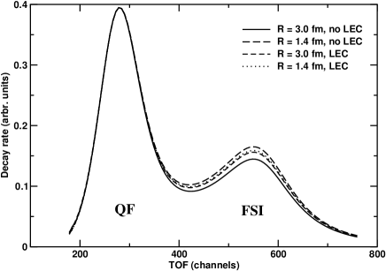
Figure 5: The $\pi^{-}d\to nn\gamma$ neutron time-of-flight distribution calculated by Gårdestig and Phillips gardestig-phillips , for two widely-separated $R$ values, without and with the low-energy constant (LEC) $\hat{d}_{1}$ contribution. The labels QF (quasi-free) and FSI indicate where the corresponding kinematics are dominant. It is in FSI that the $\hat{d}_{1}$ contribution makes a prominent effect.

As in the solar neutrino case, the $\hat{d}_{1}$ varies widely for a range of the matching radius but the result for the radiative capture process (5.70) comes out to be highly insensitive to $R$. In Fig. 5  is shown the capture rate for $R$ ranging widely from 1.4 fm to 3.0 fm. This illustrates how well the short-distance physics is captured by the simple procedure as in the $pp$ case: while the results differ appreciably for the two widely different values of $R$ without the $\hat{d}_{1}$ term in the “FSI” region, they are very close – nearly indistinguishable – when the $\hat{d}_{1}$ term is taken into account. A careful analysis of gardestig-phillips suggests that this procedure will be able to reduce the short-distance uncertainty in the determination of the $nn$ scattering length by a factor of 3 relative to the value available up to date, to, say, $\mathrel{\hbox to0.0pt{\lower 3.0pt\hbox{\hskip 1.0pt$\sim$}\hss}\raise 1.0pt\hbox{$<$}}$ 0.05 fm.

6 The EFT “completion” of SNPA

One can now pin-point how EFT comes in to $complete$ the SNPA. This can be illustrated by the results of the $hep$ process. In SNPA approaches, two-body corrections have been made in a procedure suggested a long time ago in CR71 . As discussed in hep , there are two serious problems with this procedure. The first is that without the guidance of the EFT counting rule, terms of various chiral order are mixed in at the level of computing leading-order exchange current terms. This raises the question of consistency. Since the corrections are chiral-filter unprotected, this inconsistency in chiral counting could generate serious errors. The second is more serious, having to do with the shorter-range interaction of the ${\hat{d}^{R}}$ type. In the procedure of the SNPA, short-range interactions with the range shorter than the hard-core radius $r_{c}$ are killed by short-range correlations. This simply means that roughly speaking, terms of the ${\hat{d}^{R}}$ type are missing. Without the MEEFT strategy, what enters as corrections would be largely arbitrary. One can see from Table 4 that without the balance from the ${\hat{d}^{R}}$ term, the corrections are strongly dependent on the cut-off $r_{c}$ and hence totally arbitrary, with the result differing by several factors for different cut-offs. This arbitrariness is neatly circumvented by the MEEFT procedure at the level where the calculation can be done without unknown parameters.

The ${\hat{d}^{R}}$ effect can of course be incorporated in a RigEFT with the pion field retained. Given that what matters is the proper account of the long-wavelength physics governed by chiral symmetry and of the short-distance physics subsumed in the ${\cal O}(Q^{3})$ terms, the same set of systems could be treated in a pionful RigEFT and a prediction (parameter-free) could be made. This exercise has not been done yet and it would be interesting to see to what extent the “high accuracy” in SNPA wave functions improves or worsens the prediction and to what extent there is inconsistency – if any – in chiral counting in the MEEFT procedure.

7 EFT for heavy nuclei and nuclear matter

So far we have discussed how to exploit EFT in few-nucleon systems. Can one extend the same strategy to heavier nuclei on the one hand and to nuclear matter on the other? Ultimately we would like to go to densities higher than that of nuclear matter so as to enter the regime where phase transitions to other forms of states CND2 (such as kaon condensation, quark matter etc.) are supposed to take place.

In RigEFT, one might try to approach nuclear matter by doing high-order $\chi$PT starting with a chiral Lagrangian appropriate for $n$-body systems but defined at zero density (i.e., “free space”) by systematically including diagrams involving $n$ nucleons. A possible scenario – similar in spirit to the double decimation approach mentioned below and in BR:DD – was suggested along this line by Lynn lynn which consisted of first constructing a non-topological soliton, called “chiral liquid” and then do fluctuations around the soliton. This program has not yet been successfully effectuated and it is not even clear that it is doable in practice. Now in a much more practical way, one might extend the MEEFT method we described above for few-nucleon systems to many-nucleon systems with the “realistic” two-body potentials used efficiently in the few-body problems supplemented with three-body and perhaps more-body potentials. The standard nuclear physics approach belongs to this class of approaches but, so far, without the proper incorporation of chiral symmetry. The question then is: How should one go about formulating an MEEFT that is applicable to heavy nuclei and nuclear matter?

This question is addressed elsewhere BR:DD ; BHLR06 after introducing the notion of hidden local symmetry in which vector mesons enter importantly as relevant degrees of freedom. Here we mention merely that when one approaches the nuclear matter saturation density with the intention of going beyond the nuclear matter density, it is much more astute to approach the problem via multiple decimations in the renormalization group sense rather than going in one step as one does in the standard $\chi$PT approach.

Just to illustrate the basic idea, consider the density regime near the nuclear saturation density, $n\sim 0.16$ fm^-3. (Things can become considerably subtler at higher densities.) Now what characterizes nuclear matter is the presence of the Fermi surface. It is understood that many-body interactions in the presence of Fermi surfaces generically lead – with certain exceptions that we are not concerned with here – to an RG fixed point, known as “Fermi liquid fixed point”shankar . This means that starting from a chiral Lagrangian defined at zero density, it makes a good sense to do the first decimation from the chiral scale $\Lambda_{\chi}\sim 4\pi f_{\pi}\sim 1$ GeV to the scale at which the effective interactions between nucleons in medium are defined, say, $\Lambda_{eff}\sim 2-3m_{\pi}$ and then make the second decimation to the Fermi liquid fixed point by going from $\Lambda_{eff}$ to the Fermi surface. In both of these decimations, Brown-Rho scaling (recently reviewed in BHLR06 ) is found to play an essential role. It will turn out that this procedure is consistent with the vector manifestation phenomenon of hidden local symmetry theory described in HY:PR ; BR:DD ; BHLR06 . The bridge to dense matter where chiral phase transition can take place is then made through a mapping to hidden local symmetry with the vector manifestation.

Acknowledgments

This paper, a part of the book I am writing with Chang-Hwan Lee at Pusan National University, reviews the work done over many years in collaboration with Gerry Brown, Kuniharu Kubodera, Dong-Pil Min and Tae-Sun Park to whom I am deeply indebted. The hospitality of PNU where this note was written should be acknowledged. I am very grateful for helpful comments on this note from Kuniharu Kubodera, Daniel Phillips and Steven Weinberg. Needless to say, none of my collaborators should be held responsible for possible errors or misinterpretations that I might be making here. In addition, some of the ideas developed here may not be fully shared by them.

References

- (1)
- (2) Weinberg, S., What is quantum field theory, and what did we think it is?, hep-th/9702027.
- (3) Chemtob, M. and Rho, M., Meson exchange currents in nuclear weak and electromagnetic interactins, Nucl. Phys. A163 (1971) 1.
- (4) Pieper, S.C., Wiringa, R.B. and Carlson, J., Quantum Monte Carlo calculations of excited states in A=6 - 8 nuclei, Phys. Rev. C70 (2004) 054325.
- (5) Carlson, J. and Schiavilla, R. , Structure and dynamics of few nucleon systems, Rev. Mod. Phys. 70 (1998) 743.
- (6) Pieper, S.C. and Wiringa, R.B., Quantum Monte Carlo calculations of light nuclei, Ann. Rev. Nucl. Part. Sci. 51 ((2001) 53.
- (7) Machleidt, R. and Entem, D.R., Recent advances in the theory of nuclear forces, nucl-th/0608068.
- (8) Hammer, H.W., Few-body physics in effective field theory, J. Phys. G31 (2005), S1253.
- (9) Rho, M., 10th Taiwan Lectures on “Effective field theories for nuclei, nuclear matter and dense matter,” nucl-th/0202078.
- (10) Chen, J.-W., Rupak, G. and Savage, M.J., Nucleon-nucleon effective field theory without pions, Nucl. Phys. A653 (1999) 386.
- (11) Bedaque, P.F. and van Kolck, U., Effective field theory for few nucleon systems, Ann. Rev. Nucl. Part. Sci. 52 (2002) 339.
- (12) Kaplan, D.B., Five lectures on effective field theory, nucl-th/0510023.
- (13) Wiringa, R.B., Pair counting, pion-exchange forces and the structure of light nuclei, nucl-th/0601064.
- (14) Brown, G.E., Holt, J.W., Lee, C.-H. and Rho, M., Late hadronization and matter formed at RHIC: Vector manifestation, BR scaling and hadronic freedom, Phys. Rept.. to appear; nucl-th/0608023.
- (15) Harada, M. and Yamawaki, K., Hidden local symmetry at loop: A new perspective of composite gauge bosons and chiral phase transition, Phys. Rept. 381 (2003) 1.
- (16) Weigel, H., Baryons as three flavor solitons, Int. J. Mod. Phys. A11 (1996) 2419-2544.
- (17) Jenkins, E. and Manohar, A.V., Baryon chiral perturbation theory using a heavy fermion Lagrangian, Phys. Lett. B255 (1991) 558-562.
- (18) Rho, M., Pions and the chiral bag, Prog. Part. Nucl. Phys. 8 (1982) 103.
- (19) Rho, M., Exchange currents from chiral Lagrangians, Phys. Rev. Lett. 66 (1991) 1275.
- (20) Weinberg, S., Phenomenological Lagrangians, Physica A96 (1979) 327.
- (21) Weinberg, S., Nuclear forces from chiral Lagrangians, Phys. Lett. B251(1990) 288.
- (22) Weinberg, S., Effective chiral Lagrangians for nucleon-pion interactions and nuclear forces, Nucl. Phys. B363 (1991) 3.
- (23) Nogga, A., Timmermans, R.G.E. and van Kolck, U., Renormalization of one-pion exchange and power counting, Phys. Rev. C72 (2005) 054006.
- (24) Pavon Valderrama, M. and Ruiz Arriola, E., Renormalization of the deuteron with one pion exchange, Phys. Rev. C72 (2005) 054002; Pavon Valderrama, M. and Ruiz Arriola, E., Renormalization of NN interaction with chiral two pion exchange potential: Non-central phases, nucl-th/0507075
- (25) Epelbaum, E. and Meissner, U.-G., On the renormalization of the one-pion exchange potential and the consistency of Weinberg’s power counting, nucl-th/0609037.
- (26) Kubodera, K., Delorme, J. and Rho, M., Axial currents in nuclei, Phys. Rev. Lett. 40 (1978) 755.
- (27) Chen, J.-W., Rupak, G. and Savage, M., Suppressed amplitudes in , Phys. Lett. B464 (1999) 1.
- (28) Kong, X. and Ravndal, F., Proton-proton fusion in effective field theory, Phys. Rev. C64 (2001) 044002.
- (29) Ando, S., Song, Y.-H., Park, T.-S., Fearing, H.W. and Kubodera, K., Solar-neutrino reactions on deuteron in effective field theory, Phys. Lett. B555 (2003) 49.
- (30) Park, T.-S. and Song, Y.-H., process in effective field theory, nucl-th/0311055.
- (31) Riska, D.O. and Brown, G.E., Meson exchange effects in , Phys. Lett. 38B (1973) 193-195.
- (32) Park, T.-S. et al., Parameter free effective field theory calculation for the solar proton fusion and hep processes, Phys. Rev. C67 (2003) 055206.
- (33) Wiringa, R.B., Stoks, V.G.J. and Schiavilla, R., An accurate nucleon-nucleon potential with charge independence breaking, Phys. Rev. C51 (1998) 38.
- (34) Brown, G.E. and Rho, M., Double decimation and sliding vacua in the nuclear many-body problem, Phys. Rep. 396 (2004) 1.
- (35) Park, T.-S., Min, D.-P. and Rho, M., Radiative neutron-proton capture in effective chiral Lagrangians, Phys. Rev. Lett. 74 (1995) 4153.
- (36) Park, T.-S., Min, D.-P. and Rho, M., Chiral Lagrangian approach to exchange vecor currents in nuclei, Nucl. Phys. A596 (1996) 515.
- (37) Park, B.-Y., Min, D.-P., Kubodera, K. and Rho, M., Effective field theory approach to at threshold, Phys. Lett. B472 (2002) 232.
- (38) Phillips, D.R., Chiral effective theory predictions for deutron form factor ratios at low , nucl-th/0608036.
- (39) Stoks, V. G. J., Klomp, R. A. M., Terheggen, C. P. F. and de Swart, J. J., Construction of high quality N N potential models, Phys. Rev. C49 (1994) 2950.
- (40) Machleidt, R., The high-precision, charge-dependent Bonn nucleon-nucleon potential, Phys. Rev. C63 (2001) 024001.
- (41) Park, T.-S., Kubodera. K., Min, D.-P. and Rho, M., Effective field theory for nuclei: Confronting fundamental questions in astrophysics, Nucl. Phys. A684 (2001) 101c.
- (42) Marcucci, L.E., Schiavilla, R., Viviani, M., Kievsky, A., Rosati, S. and Beacom, J.F., Weak proton capture on He-3, Phys. Rev. C63 (2001) 015801.
- (43) Super-Kamiokande Coll. (Fukuda, S. et al.) (2001) Constraints on neutrino oscillations using 1258 days of Super-Kamiokande solar neutrino data, Phys. Rev. Lett. 86 (2001) 5656.
- (44) Bahcall, J.N., Pinsonneault, M.H. and Basu, S., Solar models: Current epoch and time dependences, neutrinos, and helioseismological properties, Astrophys. J. 555 (2001) 990.
- (45) Gårdestig, A. and Phillips, D.R., How low-energy weak reactions can constrain three-nucleon forces and the neutron-neutron scattering length, Phys. Rev. Lett. 96 (2006) 232301.
- (46) E.g., Chiral nuclear dynamics: From quarks to nuclei to compact stars (World Scientific, Singapore) by Lee, C.-H. and Rho, M., to appear.
- (47) Lynn, B.W., Chiral liquids: A Theory of heavy nuclei and neutron stars, Nucl. Phys. B402 (1993) 281.
- (48) Shankar, R., Renormalization group approach to interacting fermions, Rev. Mod. Phys. 66 (1994) 129.