Angular Momentum Dependent Quark Potential of QCD Traits and Dynamical $O(4)$ Symmetry

C. B. Compean and M. Kirchbach

Abstract: A common quark potential that captures the essential traits of the QCD quark-gluon dynamics is expected to (i) interpolate between a Coulomb-like potential (associated with one-gluon exchange) and the infinite wall potential (associated with trapped but asymptotically free quarks), (ii) reproduce in the intermediary region the linear confinement potential (associated with multi-gluon self-interactions) as established by lattice QCD calculations of hadron properties. We first show that the exactly soluble trigonometric Rosen-Morse potential possesses all these properties. Next we observe that this potential, once interpreted as angular momentum dependent, acquires a dynamical $O(4)$ symmetry and reproduces exactly quantum numbers and level splittings of the non-strange baryon spectra in the $SU(2)_{I}\otimes O(4)$ classification scheme according to which baryons cling on to multi-spin parity clusters of the type $\left(\frac{K}{2},\frac{K}{2}\right)\otimes[\left(\frac{1}{2},0\right)\oplus\left(0,\frac{1}{2}\right)]$, whose relativistic image is $\psi_{\mu_{1}...\mu_{K}}$. Finally, we bring exact energies and wave functions of the levels within the above potential and thus put it on equal algebraic footing with such common potentials of wide spread as are the harmonic-oscillator– and the Coulomb potentials.

PACS: 02.30.Gp, 03.65.Ge,12.60.Jv.

1 Introduction

The non-strange baryon spectra below $\sim 2500$ MeV reveal, isospin by isospin, as a striking phenomenon mass degenerate series of $K$ pairs of resonances of opposite spatial parities and spins ranging from $\frac{1}{2}^{\pm}$ to $\left(K-\frac{1}{2}\right)^{\pm}$ which terminate by a highest spin–$\left(K+\frac{1}{2}\right)$ resonance that remains unpaired [1]. Such series (displayed in Fig. 1) perfectly fit into $SU(2)_{I}\otimes O(4)$ representations of the type $\left(\frac{K}{2},\frac{K}{2}\right)\otimes[\left(\frac{1}{2},0\right)\oplus\left(0,\frac{1}{2}\right)]$, an observation due again to [1].

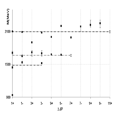
(a) (b)

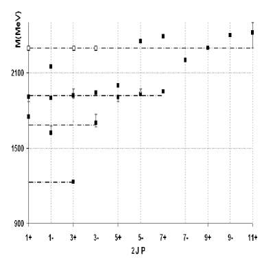
Figure 1: Experimentally observed baryon resonances (l.h.s.) $N$ and (r.h.s.) $\Delta$. The dash-point lines represent the series mass average. Notice that the resonances with masses above 2000 MeV are of significantly lower confidence but those with masses below 2000 MeV where the degeneracy is very well pronounced. Empty squares denote predicted (“missing”) states. Typical, the systematical lack of a parity partner to the first highest spins $D_{I3}$, $F_{I7}$, and $H_{I,11}$ (the last two being among the “missing” $N$ states).

The appeal of the above classification is twofold. On the one side, up to the $\Delta(1600)$ state which is likely to be a hybrid, no other resonances drop out of the proposed scheme. Also the prediction of less “missing” resonances relative to others schemes falls under this issue. On the other side, due to the local $O(4)\sim O(1,3)$ isomorphism, the non-relativistic $O(4)$ multiplets have as an exact relativistic image the covariant high-spin degrees of freedom given by the totally symmetric rank-$K$ Lorentz tensors with Dirac spinor components, $\psi_{\mu_{1}...\mu_{K}}$ known as spin-$\left(K+\frac{1}{2}\right)$ Rarita-Schwinger fields [2]. In this fashion, one can view the series of mass degenerate resonances of alternating parities and spins rising from $\frac{1}{2}^{\pm}$ to $\left(K+\frac{1}{2}\right)^{P}$ as rest frame $\psi_{\mu_{1}...\mu_{K}}$ of mass $m$ and look for possibilities to generate such multiplets as bound states within an appropriate quark potential. Although the degeneracy of the non-strange baryons follows same patterns as the states of an electron with spin in the Hydrogen atom, the level splittings are quite different. The mass formula that fits the $N(\Delta)$ spectrum has been encountered in Ref. [3] as

$$M_{(\sigma;I)}-M_{(1;I)}=-f_{I}\frac{1}{\sigma^{2}}+g_{I}\frac{\sigma^{2}-1}{4}\,, \sigma=K+1,\quad I=N,\Delta\,,$$ (1)

$$f_{N}=f_{\Delta}=600\,\,\mbox{MeV},\quad g_{N}=70\,\,\mbox{MeV}, g_{\Delta}=40\,\,\mbox{MeV}\,,$$ (2)

and contains besides the Balmer-like term, $\left(\sim-1/\sigma^{2}\right)$, also its inverse. In effect, the baryon mass splittings increase with $\sigma$. The degeneracy patterns and the mass formula have found explanation in Ref. [4] within a version of the interacting boson model (IBM) for baryons. To be specific, to the extent QCD prescribes baryons to be constituted of three quarks in a color singlet state, one can exploit for the description of baryonic systems algebraic models developed for the purposes of triatomic molecules, a path pursued by Refs. [5]. An interesting dynamical limit of the three quark system is the one where two of the quarks are “squeezed” to one independent entity, a di-quark (qq), while the third quark (q) remains spectator. In this limit, which corresponds to $U(7)\longrightarrow U(3)\times U(4)$, one can exploit the following chain of reducing $U(4)$ down to $O(2)$

$$U(4)\supset O(4)\supset O(3)\supset O(2)\,,$$

$$N\qquad\quad K\qquad\quad l\qquad\quad m\,$$ (3)

$$K=N,N-2,...1(0),\quad l=K,K-1,...,0,\quad|m|<l\,,$$ (4)

in order to describe the rotational and vibrational (rovibron) modes of the $(qq)-q$ dumbbell. In so doing, one reproduces the quantum numbers describing the degeneracies in the light quark baryon spectra by means of the following Hamiltonian:

$${\mathcal{H}}-{\mathcal{H}}_{0} = -f_{I}(4{\mathcal{C}}_{2}(so(4))+1)^{-1}+g_{I}{\mathcal{C}}_{2}(so(4))\,,$$ (5)

$${\mathcal{C}}_{2}(so(4))\left(\frac{K}{2},\frac{K}{2}\right) = \frac{(K+1)^{2}-1}{4}\left(\frac{K}{2},\frac{K}{2}\right)\,.$$ (6)

with ${\mathcal{C}}_{2}(so(4))$ being the second $so(4)$ Casimir operator. In the second row of Eq. (3) we indicate the quantum numbers associated with the respective group of the chain. Here, $N$ stands for the principle quantum number of the four dimensional harmonic oscillator associated with $U(4)$, $K$ refers to the $O(4)$ four dimensional angular momentum, while $l$, and $m$ are in turn ordinary three– and two angular momenta. In Ref. [4] the interested reader can find all the details of the algebraic description of the nucleon and $\Delta$ resonances within the rovibron limit.

Yet, as a principle challenge still remains finding a suitable quark potential that leads to the above scenario. In the present work we make the case that the exactly soluble trigonometric Rosen-Morse potential is precisely the potential we are looking for.

The paper is organized as follows. In the next section we analyze the shape of the trigonometric Rosen-Morse potential. In section III we present the exact real orthogonal polynomial solutions of the corresponding Schrödinger equation. The paper ends with a brief concluding section.

2 The shape of the trigonometric Rosen-Morse potential

We adopt the following form of the trigonometric Rosen-Morse potential [6],[7]

$$v(z)=-2b\cot z+a(a+1)\csc^{2}z\,,\quad a>-1/2,$$ (7)

displayed in Fig. 2. Here,

$$z=\frac{r}{d},\quad v(z)=V(z)/(\hbar^{2}/2md^{2}),\quad\epsilon_{n} = E_{n}/(\hbar^{2}/2md^{2})\,,$$ (8)

the one-dimensional variable is $r=|\mbox{r}|$, $d$ is a properly chosen length scale, $V(r)$ is the potential in ordinary coordinate space, and $E_{n}$ is the energy of the levels. Our point here is that $v(z)$ interpolates between a Coulomb-like and an infinite-wall potential going through an intermediary region of linear, and quadratic (harmonic-oscillator) dependences in $z$. To see this (besides inspection of Fig. 2) it is quite instructive to expand the potential in a Taylor series which for appropriately small $z$, takes the form of a Coulomb-like potential with a centrifugal-barrier like term (if $a$ were to be a positive integer) provided by the $\csc^{2}z$ part,

$$v(z)\approx-\frac{2b}{z}+\frac{a(a+1)}{z^{2}}\,.$$ (9)

In an intermediary range where inverse powers of $z$ may be neglected, one finds the linear plus a harmonic-oscillator potentials

$$v(z)\approx\frac{2b}{3}\,z+\frac{a(a+1)}{15}z^{2}\,.$$ (10)

Finally, as long as $\cot\,z\stackrel{{\scriptstyle z\to\pi}}{{\longrightarrow}}\infty$ and $\csc^{2}\,z\stackrel{{\scriptstyle z\to\pi}}{{\longrightarrow}}\infty$, the potential obviously evolves to an infinite wall.

Figure 2: The proximity of the $(\sim\cot z)$- to the $\left(\sim\frac{1}{z}\right)$ potential.

The above shape captures surprisingly well the essentials of the QCD quark-gluon dynamics where the one gluon exchange gives rise to an effective Coulomb-like potential, while the self-gluon interactions produce a linear confinement potential as established by lattice calculations of hadron properties. Finally, the infinite wall piece of the trigonometric Rosen-Morse potential provides the regime suited for trapped but asymptotically free quarks. By the above considerations one is tempted to conclude that the potential under consideration may be a good candidate for a common quark potential of QCD traits.

In the next section we present the exact solutions of the Schrödinger equation with the trigonometric Rosen-Morse potential.

3 Energies and wave functions of the levels within the trgonometric Rosen-Morse potential

The three-dimensional Schrödinger equation with the trigonometric Rosen-Morse potential (tRMP) reads:

$$\vec{\nabla}^{\,2}\ \psi(\mathbf{z})+\left(2b\cot z-\frac{a(a+1)}{\sin^{2}z}+\epsilon\right)\psi({\mathbf{z}})=0\,,$$ (11)

and is solved in polar coordinates in the standard way by separation of variables. In effect, the wave function factorizes according to

$$\psi({\mathbf{z}})=\frac{R(z)}{z}Y_{l}^{\mu}(\theta,\phi),\quad l=0,1,2,...,\quad|\mu|<l,$$ (12)

where $Y_{l}^{\mu}(\theta,\phi)$ stand for the standard spherical harmonics, and $R(z)$ satisfies the one-dimensional equation

$$\frac{d^{\,2}}{d^{2}z}\ R(z)+\left(2b\cot z-\frac{a(a+1)}{\sin^{2}z}+\epsilon\right)R(z)=0\ .$$ (13)

This equation (up to inessential notational differences) has been solved in our previous work  [8]. There, we exploited the following factorization ansatz

$$R(z)=\textrm{ e}^{-\alpha z/2}(1+\cot^{2}z)^{\frac{-(1-\beta)}{2}}C^{(\beta,\alpha)}(\cot z)\,,$$ (14)

with $\alpha$ and $\beta$ being constant parameters. Upon introducing the new variable $x=\cot z$, substituting the above factorization ansatz into Eq. (14), and a subsequent division by $(1+x^{2})^{(1-\beta)/2}$ one finds

$$(1+x^{2})\frac{d^{\,2}\ C^{(\beta,\alpha)}(x)}{d\ x^{2}}+2\left({\alpha\over 2}+\beta x\right){d\ C^{(\beta,\alpha)}(x)\over d\ x}$$

$$+{\Big{(}}(-\beta(1-\beta)-a(a+1)) + {(-\alpha(1-\beta)+2b)x+\left(\left({\alpha\over 2}\right)^{2}-(1-\beta)^{2}+\epsilon_{m}\right)\over 1+x^{2}}{\Big{)}}C^{(\beta,\alpha)}(x)=0\ .$$ (15)

This equation is suited for comparison with

$$(1+x^{2})\frac{d^{\,2}\ {\mathcal{R}}_{m}^{(\beta,\alpha)}(x)}{d\ x^{2}}+2\left({\alpha\over 2}+\beta x\right){d\ {\mathcal{R}}_{m}^{(\beta,\alpha)}(x)\over d\ x}\ -m(2\beta+m-1){\mathcal{R}}_{m}^{(\beta,\alpha)}(x)=0\,,$$ (16)

which being of the form of the text-book hypergeometric equation [9],[10],[11] can be cast into the self-adjoined Sturm-Liouville form given by

$$s(x){{d^{\,2}{\mathcal{R}}^{(\beta,\alpha)}_{m}(x)}\over{d\ x^{2}}}+{1\over{w(x)}}\left({{d\ s(x)w(x)}\over{d\ x}}\right){d\ {\mathcal{R}}^{(\beta,\alpha)}_{m}(x)\over d\ x}+\lambda_{m}\ {\mathcal{R}}^{(\beta,\alpha)}_{m}(x) = 0\ ,$$ (17)

$$s(x)=1+x^{2},\quad w^{(\beta,\alpha)}(x)=s(x)^{\beta-1}e^{-\alpha\cot^{-1}x},\,\,\lambda_{m}=-m(2\beta+m-1),\,\,-\infty<x<\infty.$$ (18)

However, while the standard textbooks consider exclusively $s(x)$ functions which are at most second order polynomials of real roots, in which case

$$w(a)s(a)x^{l}=w(b)s(b)x^{l}=0\ ,\quad\forall l=\mbox{\footnotesize integer,}$$ (19)

holds valid, the roots of $s(x)$ in Eq. (16) are imaginary. In the former case it is well known that

• ${\mathcal{R}}^{(\beta,\alpha)}_{m}(x)$ would be polynomials of order $m$,

• $\lambda_{m}$ would satisfy

  $$\lambda_{m} = -m\left(K_{1}{{d\ {\mathcal{R}}^{(\beta,\alpha)}_{1}(x)}\over{d\ x}}+{1\over 2}(m-1){{d^{\,2}s(x)}\over{d\ x^{2}}}\right)\,,$$

  with $K_{m}$ being the ${\mathcal{R}}^{(\beta,\alpha)}_{m}(x)$ normalization constant,

• the first order polynomial would be defined as

  $${\mathcal{R}}^{(\beta,\alpha)}_{1}(x)={1\over{K_{1}w(x)}}\left({{d\ s(x)w(x)}\over{d\ x}}\right)\,,$$ (21)

• the latter relation would generalize to any $m$ via the so called Rodrigues formula

  $${\mathcal{R}}^{(\beta,\alpha)}_{m}(x)=\frac{1}{K_{m}w(x)}{d^{m}\over d\ x^{m}}(w(x)\ s(x)^{m})\ ,$$ (22)

• $w(x)$ would be the weight-function with respect to which the ${\mathcal{R}}^{(\beta,\alpha)}_{m}(x)$ polynomials would appear orthogonal.

Within this context the question arises whether the imaginary roots of $s(x)=(1+x^{2})$ in Eq. (16) would prevent the ${\mathcal{R}}_{m}^{(\beta,\alpha)}(x)$ functions from being real orthogonal polynomials. The answer to this question is negative. It can be shown that also in the latter case

• the ${\mathcal{R}}_{m}^{(\beta,\alpha)}(x)$’s are polynomials of order $m$,

• they can also be constructed systematically from a Rodrigues formula in terms of the respecified weight function,

• but only a finite number them will be orthogonal due to the violation of Eq. (19).

From the historical perspective, Eq. (18) has first been brought to attention by the celebrated English mathematician Sir Edward John Routh in Ref. [12] (modulo the unessential difference in the argument of the exponential from the present $\cot^{-1}$ to Routh’s $\tan^{-1}$), the teacher of J. J. Thomson and J. Larmor, among others famous physicists. Routh observed that the weight-function of the Jacobi polynomials, $P^{(\mu,\nu)}_{m}(x)$, takes the form of Eq. (18) upon the particular complexification of the argument and the parameters according to $\mu\longrightarrow\eta=a+ib,\nu\longrightarrow\eta^{*}$, and $x\to ix$. From that he concluded that $P_{m}^{(\eta,\eta^{\ast})}(ix)$ is a real polynomial (up to a global phase factor). Later on, in 1929, the prominent Russian mathematician Vsevolod Ivanovich Romanovski, one of the founders of the Tashkent University, studied few more of their properties in [13] and it was him who observed that only a finite number of them appear orthogonal. While the mathematics literature is familiar with such polynomials [14], [15], [16], [17] where they are referred to as finite Romanovski polynomials [18], or, Romanovski-Pseudo-Jacobi polynomials [19], a curious omission from all the standard textbooks on mathematical physics [9],[10] takes place. This might be related to circumstance that the physics problems which call for such polynomials are relatively few. Recently, it has been reported in the peer physics literature [8], [20] that the Schrödinger equation with the respective hyperbolic Scarf and trigonometric Rosen-Morse potentials is resolved exactly precisely in terms of the Romanovski polynomials. Moreover, the latter are also relevant in calculation of gap probabilities in finite Cauchy random matrix ensembles [21]. In the following, we shall adopt the notion of Routh-Romanovski polynomials for obvious reasons.

3.1 The exact spectrum

Back to Eq. (15) we observe that if it is to coincide with Eq. (16) then the coefficient in front of the $1/(x^{2}+1)$ term has to nullify. This restricts the $C^{(\beta,\alpha)}(x)$ parameters in the Schrödinger wave function to be

$$-\alpha(1-\beta)+2b=0\ ,\quad\left({\alpha\over 2}\right)^{2}-(1-\beta)^{2}+\epsilon=0\,.$$ (23)

With that Eq. (15) to which one has reduced the original Schrödinger equation amounts to

$$(1+x^{2}){d^{\,2}\ C^{(\beta,\alpha)}(x)\over d\ x^{2}}+2\left({\alpha\over 2}+\beta x\right){d\ C^{(\beta,\alpha)}(x)\over d\ x}+(-\beta(1-\beta)-a(a+1))C^{(\beta,\alpha)}(x)=0\ .$$ (24)

The final step is to identify the constant term in the latter equation with the one in Eq. (16) which amounts to a third condition

$$-\beta(1-\beta)-a(a+1)=-m(2\beta+m-1)\ ,$$ (25)

which introduces the dependence of the $C^{(\beta,\alpha)}(x)$ functions on the index $m$, i.e. $C^{(\beta,\alpha)}(x)\longrightarrow C_{m}^{(\beta,\alpha)}(x)$. Remarkably, Eqs. (23) and (25) indeed allow for consistent solutions for $\alpha$, $\beta$, and $\epsilon$ and given by (upon renaming $m$ by $(n-1))$:

$$\beta_{n}=-(n+a)+1\ , \alpha_{n}={2b\over n+a}\ ,$$

$$\epsilon_{n}=(n+a)^{2}-{b^{2}\over(n+a)^{2}}\ , \quad n=m+1\,,$$ (26)

now with $n\geq 1$. In this way Eq. (26) provides the exact tRM spectrum. In effect, the polynomials that define the exact solution of the Schrödinger equation with the trigonometric Rose-Morse potential turn out identical to the Routh-Romanovski polynomials however with indices that depend on $n$. As we shall see below, this circumstance will become of crucial importance in allowing for an infinite number of orthogonal polynomials (as required by the infinite depth of the potential) and thus for avoiding the finite orthogonality of the bare Routh-Romanovski polynomials.

With that all the necessary ingredients for the solution of Eq. (24) have been prepared. In now exploiting the Rodrigues representation (when making the $n$ dependence explicit),

$$C^{(\beta_{n},\alpha_{n})}_{n}(x)\equiv{\mathcal{R}}_{n}^{(\beta_{n},\alpha_{n})}(x)={1\over K_{n}\ w^{(\beta_{n},\alpha_{n})}(x)}{d^{n-1}\over d\ x^{n-1}}\left(w^{(\beta_{n},\alpha_{n})}(x)\ s(x)^{n-1}\right)\,,$$ (27)

allows for the systematic construction of the solutions of Eq. (24). Notice that in terms of $w^{(\beta_{n},\alpha_{n})}(x)$ the wave function is expressed as

$$R_{n}^{(a,b)}(\cot^{-1}x)=\sqrt{w^{\left(-(n+a)+1,\frac{2b}{n+a}\right)}(x)}{\mathcal{R}}_{n}^{\left(-(n+a)+1,\frac{2b}{n+a}\right)}(x)\,.$$ (28)

Next one can check orthogonality of the physical solutions in $z$ space and obtain it as it should be as

$$\int_{0}^{\pi}\ R_{n}\left(z\right)R_{n^{\prime}}\left(z\right)dz=\delta_{n\ n^{\prime}}\,,$$ (29)

The orthogonality of the wave functions $R_{n}(z)$ implies in $x$ space orthogonality of the ${\mathcal{R}}_{n}^{(\beta_{n},\alpha_{n})}(x)$ polynomials with respect to $w^{(\beta_{n},\alpha_{n})}(x)\frac{dz}{dx}$ due to the variable change. As long as $\frac{d\cot^{-1}x}{dx}=-1/(1+x^{2})\equiv-1/s(x)$ then the orthogonality integral for the polynomials takes the form

$$\int_{-\infty}^{\infty}{dx\over s(x)}\sqrt{w^{(\beta_{n},\alpha_{n})}(x)}{\mathcal{R}}_{n}^{(\beta_{n},\alpha_{n})}(x)\sqrt{w^{(\beta_{n^{\prime}},\alpha_{n^{\prime}})}(x)}{\mathcal{R}}_{n^{\prime}}^{(\beta_{n^{\prime}},\alpha_{n^{\prime}})}(x)=\delta_{n\ n^{\prime}}\ .$$ (30)

The existence of an infinite number of orthogonal Routh-Romanovski polynomials was made possible on cost of the $n$ dependence of the parameters which emerged while converting the Schrödinger equation to the polynomial one.

3.2 The degeneracy in the spectra

Inspection of Eq. (26) reveals existence of an intriguing degeneracy in the tRMP spectrum. In order to see it let us assume that the $a$-parameter in Eq. (13) takes only integer non-negative $a=0,1,2,...$-values. In such a case, one immediately reads off from Eq. (26) that the energy levels for any $\sigma=(m+1+a)$ with $\sigma=1,2,3,...$ are $\sigma$-fold degenerate as $a$ can take all the values between $0$ and $(\sigma-1)$ according to $a=0,1,...(\sigma-1)$ (see Fig. 3).

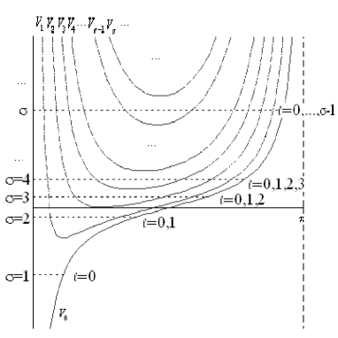
Figure 3: Degeneracy of energy levels of same $\sigma$ but different angular momenta in $l$ dependent trigonometric Rosen-Morse potentials. The curves correspond to $b=60$, a value fitted to the $N$ spectrum.

Comparison of the $a$-degeneracy to the non-strange baryon spectra in Fig. 1 and Eqs. (4) is suggestive of the idea to interpret the non-negative integer $a$-values as angular momenta and view the $\csc^{2}\left(\frac{r}{d}\right)$ term as a non-standard centrifugal barrier

$$a(a+1)\csc^{2}\left(\frac{r}{d}\right)\longrightarrow\frac{l(l+1)}{\sin^{2}\left(\frac{r}{d}\right)}\,,\quad a\equiv l=0,1,2,....$$ (31)

In terms of $\sigma$ the mass formula in Eq. (2) translates to

$$\frac{4\left(M_{\sigma,I}-M_{1,I}+\frac{1}{4}g_{I}\right)}{g_{I}}\longrightarrow\epsilon_{\sigma}=-\frac{b^{2}}{\sigma^{2}}+\sigma^{2},\quad b^{2}=\frac{4f_{I}}{g_{I}}\,.$$ (32)

Non-standard centrifugal barriers of various types have been frequently exploited in the calculation of the spectral properties of collective nuclei. Specifically, in Ref. [22] use has been made of an angular-momentum dependent potential originally suggested by Ginocchio in Refs. [23]. The non-standard centrifugal barrier in this potential asymptotically approaches for certain parameter values the physical centrifugal barrier, $l(l+1)/r^{2}$ while for another set of parameters it becomes the Pöschel-Teller potential. In our case, for small arguments the $\csc^{2}$ term also approaches the physical centrifugal term as evident from Eq. (9) and visualized by Figs. 4. Non-standard centrifugal barriers have the property to couple various multipole modes in nuclei, an example being given more recently in Ref. [24]. From now onward we shall adopt non-negative integer values for the $a$ parameter and view the $\csc^{2}$ term as a non-standard centrifugal barrier according to

$$V_{l}(r)=-2B\cot\left({r\over d}\right)+{\hbar^{2}\over 2\mu d^{2}}l(l+1)\csc^{2}\left({r\over d}\right)\,.$$ (33)

In so doing we are defining a new angular momentum dependent potential, $V_{l}(r)$, that possesses the dynamical $O(4)$ symmetry. Notice that this does not contradict the statement of Ref. [25] according to which only pure or screened Coulomb-like potentials are $O(4)$ symmetric as the theorem of Ref. [25] refers to potentials with the standard centrifugal barrier only. The $b$ parameter in Eq. (32) now relates to the potential parameter $B$ as

$$b={2\mu d^{2}B\over\hbar^{2}}\,.$$ (34)

Next we shall bring down the $a$ index, suppress the $b$ index and change notations according to

$$R^{\left((a\equiv l),b\right)}_{n}\left(\frac{r}{d}\right)\longrightarrow R_{\sigma l}\left(\frac{r}{d}\right)\,,\quad\sigma=n+l.$$ (35)

The single-particle wave functions within the angular dependent trigonometric Rosen-Morse potential are straightforwardly calculated from Eq. (28). Below we list the first three levels for illustrative purposes:

• ground state $\sigma=1$:

  $$\mbox{\bf 1s:}\quad R_{10}\left(\frac{r}{d}\right) = 2\sqrt{b(b^{2}+1)\over(1-e^{-2\pi b})}e^{-b\left(\frac{r}{d}\right)}\sin\left({\frac{r}{d}}\right),$$ (36)

• first excited state, $\sigma=2$:

  $$\mbox{\bf 2s:}\quad R_{20}\left(\frac{r}{d}\right) = \sqrt{2b\left(\left(\frac{b}{4}\right)^{2}+1\right)\over(1-e^{-\pi b})}e^{-b\left(\frac{r}{2d}\right)}\sin{\left(\frac{r}{d}\right)}\left(b\sin\left(\frac{r}{d}\right)-2\cos\left(\frac{r}{d}\right)\right),$$

  $$\mbox{\bf 2p:}\quad R_{21}\left(\frac{r}{d}\right) = 2\sqrt{2\over 3}\sqrt{b\left(\left(\frac{b}{2}\right)^{2}+1\right)\left(\left(\frac{b}{4}\right)^{2}+1\right)\over(1-e^{-\pi b})}e^{-b\frac{r}{2d}}\sin^{2}\left(\frac{r}{d}\right),$$ (37)

• second excited state $\sigma=3$:

  $$\mbox{\bf 3s:}\quad R_{30}\left(\frac{r}{d}\right)) = \frac{2}{9\sqrt{3}}\sqrt{\frac{\left(b\left(\frac{b}{9}\right)^{2}+1\right)}{\left(1-e^{-2\pi\frac{b}{3}}\right)}}e^{-b\frac{r}{3d}}\sin\left(\frac{r}{d}\right)$$

  $$\left(2\left(\left({b\over 3}\right)^{2}\sin^{2}\left({r\over d}\right)-b\sin\left({r\over d}\right)\cos\left({r\over d}\right)+\cos^{2}\left({r\over d}\right)\right)-1\right),$$

  $$\mbox{\bf 3p:}\quad R_{31}\left(\frac{r}{d}\right) = \left({2\over 3}\right)^{\frac{3}{2}}\sqrt{b\left(\left(\frac{b}{3}\right)^{2}+1\right)\left(\left(\frac{b}{9}\right)^{2}+1\right)\over(1-e^{-2\pi\frac{b}{3}})}e^{-b\frac{r}{3d}}\sin^{2}\left({\frac{r}{d}}\right)\left(b\sin\left(r\over d\right)-6\cos\left(r\over d\right)\right),$$

  $$\mbox{\bf 3d:}\quad R_{32}\left(\frac{r}{d}\right) = 4\sqrt{2\over 15}\sqrt{b\left(\left(\frac{b}{3}\right)^{2}+1\right)\left(\left(\frac{b}{6}\right)^{2}+1\right)\left(\left(\frac{b}{9}\right)^{2}+1\right)\over(1-e^{-2\pi\frac{b}{3}})}e^{-b\frac{r}{3d}}\sin^{3}\left({\frac{r}{d}}\right).$$ (38)

In Figs. 5 we display as an illustrative example the wave functions for the first two $\sigma$ levels.

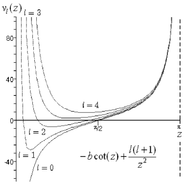
(a) (b)

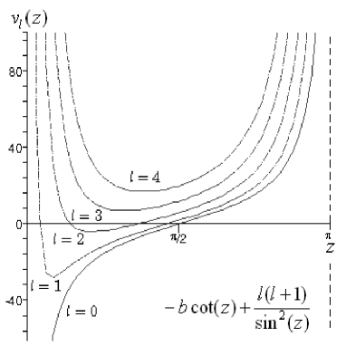
Figure 4: The $\cot\left(\frac{r}{d}\right)$ potential with the physical centrifugal barrier (left) and the non-standard one (right).

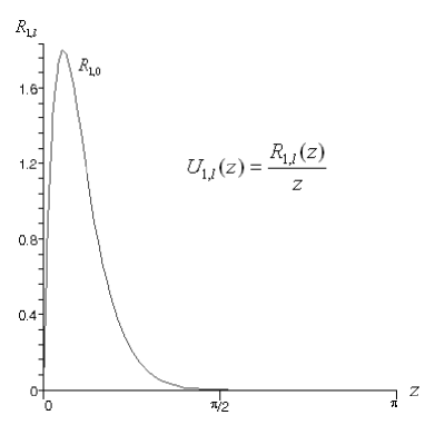
(a) (b)

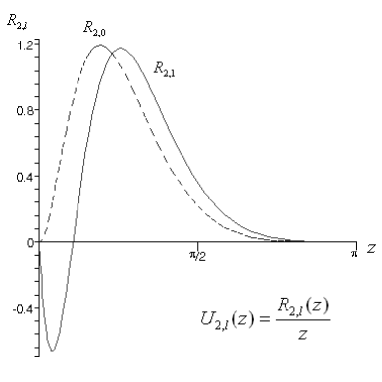
Figure 5: Wave functions for $\sigma=1,l=0$ (left) and $\sigma=2,l=0,1$ (right).

4 Discussion and concluding remarks

In this work we made the case that the trigonometric Rosen-Morse potential with the $\csc^{2}$ term being reinterpreted as a non-standard centrifugal barrier provides quantum numbers and level splittings of same dynamical $O(4)$ patterns as observed within the $SU(2)_{I}\times O(4)$ classification scheme of baryons in the light quark sector. Due to local $O(4)\sim O(1,3)$ isomorphism, the potential $\left(\frac{K}{2},\frac{K}{2}\right)\otimes[\left(\frac{1}{2},0\right)\oplus\left(0,\frac{1}{2}\right)]$ levels have as a relativistic image the covariant field theoretical high-spin degrees of freedom, $\psi_{\mu_{1}...\mu_{K}}$.

We presented exact energies and wave functions of a particle within the above potential and in so doing put it on equal algebraic footing with the harmonic oscillator and/or the Coulomb potentials of wide spread. In this fashion,

• an element of covariance was brought into the otherwise non-covariant potential picture,

• the algebraic Hamiltonian in Eq. (6) describing the $O(4)$ degeneracy in the $N$ and $\Delta$ spectra was translated into a potential model of same dynamical symmetry.

The $O(4)$ degeneracy of the $N$ and $\Delta$ spectra seem to speak in favor of quark-diquark as leading configurations of resonance structures. Yet, form factors are known to be more sensitive to configuration mixing effects and may require inclusion of genuine three quark configurations. As long as the tRMP shape captures the essential traits of the quark-gluon dynamics of QCD, we here consider it as a promising candidate for a realistic common quark potential that is worth being employed in the calculations of spectroscopic properties of non-strange resonances.

References

- [1] M. Kirchbach, Mod. Phys. Lett. A 12, 2373-2386 (1997).
- [2] W. Rarita, J. Schwinger, Phys. Rev. 60, 61 (1941).
- [3] M. Kirchbach, Int. J. Mod. Phys. A 15, 1435-1451 (2000).
- [4] M. Kirchbach, M. Moshinsky, Yu. F. Smirnov, Phys. Rev. D 64 , 114005 (2001).
- [5] R. Bijker, F. Iachello, A. Leviatan, Ann. Phys. 236, 69-116 (1994).
- [6] C. V. Sukumar, J. Phys. A:Math. Gen. 18, 2917 (1998); C. V. Sukumar, AIP proceedings 744, eds. R. Bijker et al., Supersymmetries in physics and applications (New York, 2005) p. 167.
- [7] F. Cooper, A. Khare, U. P. Sukhatme, Supersymmetry in Quantum Mechanics (World Scientific, Singapore, 2001).
- [8] C. B. Compean, M. Kirchbach, J. Phys. A:Math.Gen. 39, 547 (2006).
- [9] M. Abramowitz, I. A. Stegun, Handbook of Mathematical Functions with Formulas, Graphs and Mathematical Tables, (Dover, 2nd edition, New York, 1972).
- [10] G. B. Arfken, H. J. Weber, Mathematical Methods for Physicists, 6th ed. (Elsevier-Academic Press, Amsterdam, 2005).
- [11] Phylippe Dennery, André Krzywicki, Mathematics for Physicists (Dover, New York, 1996).
- [12] E. J. Routh, Proc. London Math. Soc. 16 245 (1884).
- [13] V. I. Romanovski, C. R. Acad. Sci. Paris, 188, 1023 (1929).
- [14] A. F. Nikiforov, V. B. Uvarov, Special Functions of Mathematical Physics (Birkhäuser, Basel-Boston, 1988).
- [15] M. E. H. Ismail, Classical and Quantum Orthogonal Polynomials in One Variable (Cambridge Univ. Press, 2005).
- [16] W. Koepf, M. Masjed-Jamei, Integral Transforms and Special Functions, 17, 559 (2006).
- [17] Yu. A. Neretin, Beta-Integrals and Finite Orthogonal Systems of Wilson Polynomials, E-Print Archive: math.CA/0206199.
- [18] Alejandro Zarzo Altarejos, Differential Equations of the Hypergeometric Type (in Spanish), Ph. D. thesis, Faculty of Science, University of Granada (1995).
- [19] P. A. Lesky, Sitzungsberichte der Mathematisch-Naturwissenschftlichen Klasse Abt. II, Österreichische AdW, 206, 127 (1997).
- [20] D. E. Alvarez-Castillo, M. Kirchbach, Exact Spectrum and Wave Functions of the Hyperbolic Scarf Potential in Terms of Finite Romanovski Polynomials , E-Print Archive: quant-ph/0603122, v3.
- [21] N. Witte, P. J. Forrester, Nonlinearity 13, 1965 (2000); E-Print Archive: math-ph/0009022.
- [22] K. Bennaceur, J. Dobachewski, M. Ploszajczak, Phys. Rev. C 60, 034308 (1999).
- [23] J. N. Ginocchio, Ann. Phys. (N.Y.) 152, 203 (1984); 159, 467 (1985).
- [24] N. Minkov, P. Jotov, S. Drenska, W. Scheid, D. Bonatsos, D. Lenis, D. Petrellis, Nuclear collective motion with a coherent coupling between quadrupole and octupole modes, E-Print Archive: nucl-th/0603059.
- [25] Bei Zeng, Jin-Yan Zeng, J. Math. Phys. 43, Issue 2, 897 (2002).