Parity-Violating Observables of Two-Nucleon Systems in Effective Field Theory

Abstract

A newly-proposed parity-violating nucleon-nucleon interaction based on effective field theory is studied in this work. It is found that at low energy, i.e., $E_{\mathrm{lab}}\lesssim 90\,\mbox{MeV}$ for ${}^{1}S_{0}$–${}^{3}P_{0}$ transitions and $E_{\mathrm{lab}}\lesssim 40\,\mbox{MeV}$ for ${}^{3}S_{1}$–${}^{1}P_{1}$ and ${}^{3}S_{1}$–${}^{3}P_{1}$ transitions, the parity-violating observables can be completely specified by a minimal set of six parameters. It contains five low-energy constants, which are equivalent to the Danilov parameters, and an additional parameter that characterizes the long-range one-pion exchange and is proportional to the parity-violating pion-nucleon coupling constant $h_{\pi}^{1}$. Selected observables in two-nucleons systems are analyzed in this framework with their dependence on these parameters being expressed in a nearly model-independent way.

I Introduction

Study of the parity-violating (PV) nucleon-nucleon ($NN$) interaction, $V^{\textrm{PV}}$, and its associated nuclear PV phenomena begins with the report by Tanner Tanner (1957) shortly after the parity violation was confirmed experimentally in 1957. The first clear evidence is found a decade after by observing a non-zero circular polarization in the $\gamma$-decay of ${}^{181}\textrm{Ta}$ Lobashov et al. (1967). Although quite a few PV observables have been measured later on in various nuclear systems, ranging from simple two-body scattering to heavy nuclear reaction, our current understanding of nuclear parity violation is still far from complete (see, e.g., Refs. Adelberger and Haxton (1985); Haeberli and Holstein (1995); Desplanques (1998); Ramsey-Musolf and Page (2006) for reviews of this field). The major difficulty is two-fold: not only these experiments require high precision to discern the much smaller PV signals, but also in theory, the non-perturbative character of the quark-gluon dynamics makes a “first-principle” formulation of $V^{\textrm{PV}}$ as yet impossible. Despite the difficulties and that the underlying theory, the $SU(2)\otimes U(1)$ gauge theory, is well-established, the study of $V^{\textrm{PV}}$ is still valuable for two main reasons. First, it is the only viable venue to observe the neutral weak current interaction between two quarks at low energy. Second, it supplies more information about the nucleon-nucleon ($NN$) dynamics in addition to existing scattering data.

The phenomenological development of $V^{\textrm{PV}}$ proceeds in a similar fashion as what has been achieved in the parity-conserving (PC) $NN$ interaction—starting out from pure phase-shift analyses, then parameterizations in meson exchange models, and finally to rigorous effective field theory (EFT) formulation nowadays. It is first pointed out by Danilov Danilov (1965, 1971, 1972) that, at low energy, $V^{\textrm{PV}}$ can be characterized by five $S\textrm{--}P$ scattering amplitudes: $\lambda_{s}^{pp}$, $\lambda_{s}^{np}$, and $\lambda_{s}^{nn}$ for ${}^{1}S_{0}\textrm{--}^{3}P_{0}$ transitions, $\lambda_{t}$ for ${}^{3}S_{1}\textrm{--}^{1}P_{1}$ transition, and $\rho_{t}$ for ${}^{3}S_{1}\textrm{--}^{3}P_{1}$ transition. This idea is generalized by Desplanques and Missimer Desplanques and Missimer (1978, 1979) to an effective version—through the Bethe-Goldstone equation—which applies to many-body systems. On the other hand, formulations of $V^{\textrm{PV}}$ in terms of meson exchange models can be dated back to the seminal works by Blin-Stoyle Blin-Stoyle (1960a, b) and Barton Barton (1961). The specific form involving one $\pi$-, $\rho$-, and $\omega$-exchanges, $V_{\textrm{OME}}^{\textrm{PV}}$, then becomes the standard in this field after Desplanques, Donoghue, and Holstein (DDH) give their prediction of the six PV meson-nucleon coupling constants, $h_{m}^{i}$’s ($m$ denotes the type of meson and $i$ the isospin), based on a quark model calculation Desplanques et al. (1980).  As explained in Ref. Adelberger and Haxton (1985), $V_{\textrm{OME}}^{\textrm{PV}}$ has a close connection to the $S\textrm{--}P$ amplitude formulation, $V_{S\textrm{--}P}^{\textrm{PV}}$, at low energy: The amplitude $\rho_{t}$ contains a long-range one-pion-exchange contribution, and the other amplitudes, including the short-range part of $\rho_{t}$, are all related to the vector-meson exchanges.

Most of the existing PV observables have been analyzed in the one-meson-exchange (OME) framework. However, a consistent constraint of the PV coupling constants is not realized yet. There are several reasons. On the experimental side, many data have large errors so are not very constrictive; also, these observables in terms of $h_{m}^{i}$’s are not independent enough to allow a simultaneous determination of these six parameters. On the theoretical side, several precise data involve many-body systems; the reliabilities of these calculations are questionable. As one can see from, e.g., Refs. Haeberli and Holstein (1995); Haxton et al. (2001, 2002), a two-dimensional constraint on the particular linear combinations of the isoscalar and isovector couplings already shows some discrepancy. Besides these possibilities, one might also wonder if the analysis framework, i.e., $V_{\textrm{OME}}^{\textrm{PV}}$, could be the culprit.

To address the last question, Zhu et al. Zhu et al. (2005) recently reformulate $V^{\textrm{PV}}$ in the EFT framework to the order of $Q$ ($Q$ is the momentum scale). This new framework comes with two incarnations: one with pions fully integrated out, $V_{\not{\pi}}^{\textrm{PV}}$, and the other with dynamical pions, $V_{\textrm{EFT}}^{\textrm{PV}}$. The pionless version, thought to be suitable for low-energy cases with $E_{\textrm{lab}}\lesssim 100\,\textrm{MeV}$, only contains the short-range (SR) interaction, $V_{1,\,\textrm{SR}}^{\textrm{PV}}$, and it is specified by ten low-energy constants (LECs). However, as Zhu et al. argued semi-quantitatively, only five of them are truly independent at low energy, and can be mapped to the five $S\textrm{--}P$ amplitudes. In the pionful version, dynamical pions generate two explicit terms: the leading-order, long-range (LR) interaction, $V_{-1,\,\textrm{LR}}^{\textrm{PV}}$, due to the one-pion exchange (OPE), and the subleading-order, medium-range (MR) interaction, $V_{1,\,\textrm{MR}}^{\textrm{PV}}$, due to the two-pion exchange (TPE). While the OPE part is also familiar in $V_{\textrm{OME}}^{\textrm{PV}}$, the TPE part has never been systematically treated before. By considering vertex corrections to the OPE term, the original formulation by Zhu et al. contains an extra next-to-next-to-leading-order interaction, $V_{1,\,\textrm{LR}}^{\textrm{PV}}$, whose operator structure is thought to be different from others already being specified. This term has recently been shown as redundant Liu and Ramsey-Musolf , so will be ignored in our discussion. Overall, in addition to the $10$ LECs in the SR interaction, the pionful theory introduces, to $\mathcal{O}(Q)$, two more parameters: one with the interaction ($h_{\pi}^{1}$) and the other with the pion-exchange current ($\bar{c}_{\pi}$). An important point to note is that, although $V_{1,\,\textrm{SR}}^{\textrm{PV}}$ takes the same form in both $V_{\mathrm{EFT}}^{\textrm{PV}}$ and $V_{\not{\pi}}^{\textrm{PV}}$, the LECs in these two EFT frameworks have different meanings: all the pion physics is included in LECs for the pionless version; but it is singled out in the pionful version.

With the advance of experimental techniques showing promise of PV measurements in few-body systems—where reliable theoretical calculations are available—an extensive search program to re-analyze PV observables is sketched in Ref. Zhu et al. (2005). The key of this re-analysis is to use the “hybrid” EFT framework, which combines the state-of-the-art wave functions (from phenomenological potential-model calculations) and the most general form of $V^{\textrm{PV}}$(from EFT techniques). The immediate goal is to find out whether a more consistent picture of nuclear parity violation can be reached among few-body systems. The long-term goal of including other precise measurements in many-body systems certainly relies on the previous success.

This paper takes the first step dealing with two-nucleon systems at low energy. The aim is to express the observables, both existing and potentially possible, in terms the EFT parameters, and to serve as a part of the database which the complete search program calls for. The general formalism is introduced in Sec. II. The connection between $V^{\mathrm{PV}}$ (both $V_{\not{\pi}}^{\textrm{PV}}$ and $V_{\mathrm{EFT}}^{\mathrm{PV}}$) and the $S$–$P$ amplitudes is studied in Sec. III. To facilitate a both realistic and economic search program, special attention is on the quantitative determination of a minimal set of parameters and its applicable energy range. The observables of two-nucleon systems are discussed subsequently in Sec. IV, and a summary follows in Sec. V.

II Formalism 

A fully consistent study of nuclear PV phenomena in the EFT framework requires treating PC and PV interactions order by order on the same footing. On the other hand, the “hybrid” approach, which combines the state-of-the-art wave functions from phenomenology and the general operator structure from EFT, is shown to have quite some success. In this work, we follow the latter approach as outlined in Ref. Zhu et al. (2005).

II.1 Parity-Conserving Potential and Wave Functions

In the hybrid EFT framework, the unperturbed scattering and deuteron (the binding energy $E_{\mathcal{D}}\cong 2.22\,\textrm{MeV}$) wave functions, $\ket{\psi}^{(\pm)}$ and $\ket{\psi}_{\mathcal{D}}$, are obtained by solving the Lippmann-Schwinger and Schrödinger equations, respectively,

$$(H_{0}+V^{\textrm{PC}}\mp i\,\epsilon)\ket{\psi}^{(\pm)} =E\ket{\psi}^{(\pm)}\,,$$ (1)

$$(H_{0}+V^{\textrm{PC}})\ket{\psi}_{\mathcal{D}} =-E_{\mathcal{D}}\ket{\psi}_{\mathcal{D}}\,,$$ (2)

with a chosen high-quality phenomenological potential as $V^{\textrm{PC}}$. In this work, we use Argonne $v_{18}$ (AV18) Wiringa et al. (1995) model exclusively. The model dependence of PV observables on strong potentials has been extensively studied in Refs. Carlson et al. (2002); Schiavilla et al. (2004); for most cases, no strong deviation from AV18 is found.

Since the PV interaction is small, we treat it as a first-order perturbation. The PV scattering amplitude, $\widetilde{M}$, is obtained by the first-order distorted-wave Born approximation

$$\widetilde{M}=^{(-)}\bra{\psi}V^{\textrm{PV}}\ket{\psi}^{(+)}\,.$$ (3)

The parity admixtures of the scattering and deuteron states, $\widetilde{\ket{\psi}}^{(\pm)}$ and $\widetilde{\ket{\psi}}_{\mathcal{D}}$, are obtained by solving the inhomogeneous differential equations

$$(E-H_{0}-V^{\textrm{PC}})\widetilde{\ket{\psi}}^{(\pm)} =V^{\textrm{PV}}\ket{\psi}^{(\pm)}\,,$$ (4)

$$(E_{\mathcal{D}}+H_{0}+V^{\textrm{PC}})\widetilde{\ket{\psi}}_{\mathcal{D}} =-V^{\textrm{PV}}\ket{\psi}_{\mathcal{D}}\,,$$ (5)

respectively, where the product of the PV potential and the unperturbed wave function serves as the source term. We refer more technical details regarding the partial wave expansion, phase shifts, and numerical procedures to Refs. Carlson et al. (2002); Schiavilla et al. (2004); Liu et al. (2003), but only mention a subtle point about the phase convention: We adopt, exclusively, the Condon-Shortley phase convention; it is different from the Biedenharn-Rose phase convention which contains an additional phase $i^{L}$ for the partial wave of orbital angular momentum $L$.

II.2 Parity-Violating Interaction in Pionless EFT

In the pionless EFT, the PV interaction is entirely short-range and takes the following form in the coordinate space Zhu et al. (2005)

$$V_{\not{\pi}}^{\textrm{PV}}(\bm{r}) =V_{1,\textrm{SR}}^{\textrm{PV}}(\bm{r})$$

$$=\frac{2}{\Lambda_{\chi}^{3}}\,\left\{\left[C_{1}+(C_{2}+C_{4})\,\tau_{+}^{z}+C_{3}\,\tau_{\cdot}+C_{5}\,\tau^{zz}\right]\,\bm{\sigma}_{-}\cdot\bm{y}_{m+}(\bm{r})\right.$$

$$\quad+\left[\widetilde{C}_{1}+(\widetilde{C}_{2}+\widetilde{C}_{4})\,\tau_{+}^{z}+\widetilde{C}_{3}\,\tau_{\cdot}+\widetilde{C}_{5}\,\tau^{zz}\right]\,\bm{\sigma}_{\times}\cdot\bm{y}_{m-}(\bm{r})$$

$$\quad+\left.(C_{2}-C_{4})\,\tau_{-}^{z}\,\bm{\sigma}_{+}\cdot\bm{y}_{m+}(\bm{r})+\widetilde{C}_{6}\,\tau_{\times}^{z}\,\bm{\sigma}_{+}\cdot\bm{y}_{m-}(\bm{r})\right\}\,,$$ (6)

where $\Lambda_{\chi}$ is the scale of chiral symmetry breaking and related to the pion decay constant $F_{\pi}$ by $\Lambda_{\chi}=4\,\pi\,F_{\pi}\approx 1.161\,\textrm{GeV}$; $\tau_{\cdot}\equiv\bm{\tau}_{1}\cdot\bm{\tau}_{2}$, $\tau_{\pm}^{z}\equiv(\tau_{1}^{z}\pm\tau_{2}^{z})/2$, $\tau_{\times}^{z}\equiv i\,(\bm{\tau}_{1}\times\bm{\tau}_{2})^{z}/2$, and $\tau^{zz}\equiv\left(3\,\tau_{1}^{z}\,\tau_{2}^{z}-\bm{\tau}_{1}\cdot\bm{\tau}_{2}\right)/(2\,\sqrt{6})$ are the isospin operators;  $\bm{\sigma}_{\pm}\equiv\bm{\sigma}_{1}\pm\bm{\sigma}_{2}$ and $\bm{\sigma}_{\times}\equiv i\,\bm{\sigma}_{1}\times\bm{\sigma}_{2}$ are the spin operators. The spatial operator $\bm{y}_{m-(+)}(\bm{r})$ is defined as the (anti-) commutator of $-i\,\bm{\nabla}$ with the $\textrm{mass}^{2}$-weighted Yukawa function $f_{m}(r)$

$$\bm{y}_{m\pm}(\bm{r})=[-i\,\bm{\nabla}\,,\,f_{m}(r)]_{\pm}\equiv\left[-i\,\bm{\nabla}\,,\,m^{2}\,\frac{\textrm{e}^{-m\,r}}{4\,\pi\,r}\right]_{\pm}\,.$$ (7)

When $m\rightarrow\infty$, $f_{m}(r)\rightarrow\delta(r)/r^{2}$; the potential thus takes a four-fermion contact form as expected.

While using a Yukawa functional form for $f_{m}(r)$ leads to a similar spatial behavior as the conventional $V_{\textrm{OME}}^{\textrm{PV}}$, other choices—as long as they are realized in the context of EFT—are also possible. For instance, taking into account the monopole form factors at both the strong and weak vertices with a cutoff $\Lambda_{m}$, one obtains a modified Yukawa function

$$\bar{f}_{m}(r)=\frac{m^{2}}{4\,\pi\,r}\,\left\{\textrm{e}^{-m\,r}-\textrm{e}^{-\Lambda_{m}\,r}\left[1+\frac{1}{2}\,(1-\frac{m^{2}}{\Lambda_{m}^{2}})\,\Lambda_{m}\,r\right]\right\}\,.$$ (8)

At the $\Lambda_{m}\rightarrow\infty$ limit, $\bar{f}_{m}(r)$ recovers the “bare” Yukawa form $f_{m}(r)$. We note that in Refs. Carlson et al. (2002); Schiavilla et al. (2004), a recent and extensive OME analyses of two-body nuclear PV, the authors adopt $\bar{f}_{m}(r)$ instead of the conventional choice $f_{m}(r)$.

As $\widetilde{C}_{2}$ and $\widetilde{C}_{4}$ appear as a linear combination $\widetilde{C}_{2}+\widetilde{C}_{4}$ in Eq. (6), $V_{1,\mathrm{SR}}^{\textrm{PV}}$ contains $11-1=10$ LECs. After resolving the isospin and spin matrix elements of all allowed two-nucleon states, the PV observables depend on the following ten linear combinations of $C$’s and $\widetilde{C}$’s:

• $p\,p$ : $D_{v}^{pp}=C_{1}+C_{3}+C_{2}+C_{4}+C_{5}/\sqrt{6}$ and $\widetilde{D}_{v}^{pp}=\widetilde{C}_{1}+\widetilde{C}_{3}+[\widetilde{C}_{2}+\widetilde{C}_{4}]+\widetilde{C}_{5}/\sqrt{6}$,

• $n\,n$ : $D_{v}^{nn}=C_{1}+C_{3}-C_{2}-C_{4}+C_{5}/\sqrt{6}$ and $\widetilde{D}_{v}^{nn}=\widetilde{C}_{1}+\widetilde{C}_{3}-[\widetilde{C}_{2}+\widetilde{C}_{4}]+\widetilde{C}_{5}/\sqrt{6}$,

• $n\,p\,|_{T_{i}=T_{f}=1}$ : $D_{v}^{np}=C_{1}+C_{3}-2\,C_{5}/\sqrt{6}$ and $\widetilde{D}_{v}^{np}=\widetilde{C}_{1}+\widetilde{C}_{3}-2\,\widetilde{C}_{5}/\sqrt{6}$,

• $n\,p\,|_{T_{i}=T_{f}=0}$ : $D_{u}=C_{1}-3\,C_{3}$ and $\widetilde{D}_{u}=\widetilde{C}_{1}-3\,\widetilde{C}_{3}$,

• $n\,p\,|_{T_{i}\neq T_{f}}$ : $D_{w}=C_{2}-C_{4}$ and $\widetilde{D}_{w}=\widetilde{C}_{6}$.

In fact, $V_{1,\mathrm{SR}}^{\textrm{PV}}$ is tantamount to the $\rho$- and $\omega$-sectors of $V_{\textrm{OME}}^{\textrm{PV}}$ if one assumes i) $m_{\rho}=m_{\omega}=m$ and ii) the following relations between $\widetilde{C}$’s and $C$’s:

$$\frac{\widetilde{C}_{1}}{C_{1}}=\frac{\widetilde{C}_{2}}{C_{2}} =1+\chi_{\omega}\,,$$ (9a)

$$\frac{\widetilde{C}_{3}}{C_{3}}=\frac{\widetilde{C}_{4}}{C_{4}}=\frac{\widetilde{C}_{5}}{C_{5}} =1+\chi_{\rho}\,,$$ (9b)

where $\chi_{\omega}$ and $\chi_{\rho}$ are the isoscalar and isovector strong tensor couplings, respectively. The remaining $11-5=6$ independent LECs in EFT then have a one-to-one mapping to the PV heavy-meson-nucleon coupling constants as

$$(C_{1},\,C_{2}) \rightarrow-\frac{g_{\omega}}{2}\,(h_{\omega}^{0},\,h_{\omega}^{1})\,\frac{\Lambda_{\chi}^{3}}{m_{\scriptscriptstyle{N}}\,m_{\omega}^{2}}\,,$$ (10a)

$$(C_{3},\,C_{4},\,C_{5},\,\widetilde{C}_{6}) \rightarrow-\frac{g_{\rho}}{2}\,(h_{\rho}^{0},\,h_{\rho}^{1},\,h_{\rho}^{2},\,h_{\rho}^{1^{\prime}})\,\frac{\Lambda_{\chi}^{3}}{m_{\scriptscriptstyle{N}}\,m_{\rho}^{2}}\,,$$ (10b)

where $g_{x}$ denotes the strong $x$-meson-nucleon coupling constant. Note that in analyses based on $V_{\textrm{OME}}^{\textrm{PV}}$, the $h_{\rho}^{1^{\prime}}$ part is usually ignored because it has the same operator structure as the LR OPE interaction, i.e., the $h_{\pi}^{1}$ part, but a very small predicted value for $h_{\rho}^{1^{\prime}}$. One might be tempted to adopt a different Yukawa mass $m=m_{\pi}$ for the $\widetilde{C}_{6}$ term so that $V_{1,\mathrm{SR}}^{\textrm{PV}}$ bears even more similarity to $V_{\textrm{OME}}^{\textrm{PV}}$. However, this is undesirable from the EFT point of view because two quite different length scales, $1/m_{\rho}$ and $1/m_{\pi}$, both show up in the “short-range” interaction.

II.3 Parity-Violating Interaction in Pionful EFT

When pions are treated explicitly, the EFT PV interaction, as formulated in Ref. Zhu et al. (2005), contains three parts 

$$V_{\textrm{EFT}}^{\textrm{PV}}(\bm{r})=V_{-1,\textrm{LR}}^{\textrm{PV}}(\bm{r})+V_{1,\textrm{MR}}^{\textrm{PV}}(\bm{r})+V_{1,\textrm{SR}}^{\textrm{PV}}(\bm{r})\,.$$ (11)

The leading term $V_{-1,\textrm{LR}}^{\textrm{PV}}$ is the familiar PV OPE potential

$$V_{-1,\textrm{LR}}^{\textrm{PV}}(\bm{r})=\frac{2}{\Lambda_{\chi}^{3}}\,\widetilde{C}_{6}^{\pi}\,\tau_{\times}^{z}\,\bm{\sigma}_{+}\cdot\bm{y}_{\pi-}(\bm{r})\,,$$ (12)

with

$$\widetilde{C}_{6}^{\pi}=\frac{h_{\pi}^{1}\,g_{A}}{2\,\sqrt{2}}\,\frac{\Lambda_{\chi}^{3}}{F_{\pi}\,m_{\pi}^{2}}=\frac{h_{\pi}^{1}\,g_{\pi}}{2\,\sqrt{2}}\,\frac{\Lambda_{\chi}^{3}}{m_{\scriptscriptstyle{N}}\,m_{\pi}^{2}}\,,$$ (13)

where $g_{A}=1.27$ is the nucleon axial vector coupling constant and $m_{\pi}=139.57\,\textrm{MeV}$; and the second equality follows from the Goldberger-Trieman relation.

The subleading MR interaction is due to TPE and has the form 

$$V_{1,\textrm{MR}}^{\textrm{PV}}(\bm{r})= \frac{2}{\Lambda_{\chi}^{3}}\,\Big{\{}\widetilde{C}_{2}^{2\pi}\,\tau_{+}^{z}\,\bm{\sigma}_{\times}\cdot\bm{y}_{2\pi}^{L}(\bm{r})$$

$$+\widetilde{C}_{6}^{2\pi}\,\tau_{\times}^{z}\,\bm{\sigma}_{+}\cdot\left[\left(1-1/(3\,g_{A}^{2})\right)\,\bm{y}_{2\pi}^{L}(\bm{r})-1/3\,\bm{y}_{2\pi}^{H}(\bm{r})\right]\Big{\}}\,,$$ (14)

with

$$\widetilde{C}_{2}^{2\pi} =-4\,\sqrt{2}\,\pi\,g_{A}^{3}\,h_{\pi}^{1}\,,$$ (15)

$$\widetilde{C}_{6}^{2\pi} =3\,\sqrt{2}\,\pi\,g_{A}^{3}\,h_{\pi}^{1}\,.$$ (16)

The Yukawa-like radial functions $f_{2\pi}^{L}(r)$ and $f_{2\pi}^{H}(r)$, for generating $\bm{y}_{2\pi}^{L}(\bm{r})$ and $\bm{y}_{2\pi}^{H}(\bm{r})$ via Eq. (7), are obtained from the Fourier transforms of

$$L(q) =\frac{\sqrt{4\,m_{\pi}^{2}+\bm{q}^{2}}}{|\bm{q}|}\,\ln\left(\frac{\sqrt{4\,m_{\pi}^{2}+\bm{q}^{2}}+|\bm{q}|}{2\,m_{\pi}}\right)\,,$$ (17)

$$H(q) =\frac{4\,m_{\pi}^{2}}{4\,m_{\pi}^{2}+\bm{q}^{2}}\,L(q)\,,$$ (18)

respectively. In Fig. 1, the plots of $r\,f_{2\pi}^{L}(r)$ and $r\,f_{2\pi}^{H}(r)$ are shown with several dipole cutoff factors $(\Lambda^{2}-4m_{\pi}^{2})^{2}/(\Lambda^{2}+q^{2})^{2}$—including the bare case, i.e., $\Lambda\rightarrow\infty$—introduced in the Fourier transforms. As one clearly sees, the short distance behaviors are quite cutoff-sensitive, especially for $f_{2\pi}^{L}(r)$ since $L(q)$ diverges logarithmically as $\ln q/m_{\pi}$. On the other hand, the long-range tails, roughly decrease like $e^{-1.58\,r}$ and $e^{-1.47\,r}$, track well with $e^{-2\,m_{\pi}\,r}=e^{-1.41\,r}$.

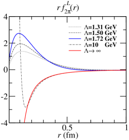
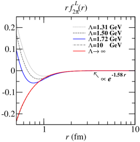
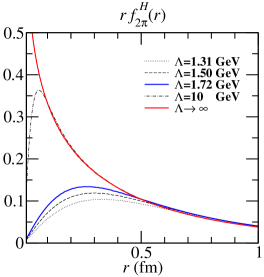
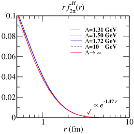
Figure 1: The $r$-weighted Yukawa-like radial functions $r\,f_{2\pi}^{L}(r)$ and $r\,f_{2\pi}^{H}(r)$ in the two-pion-exchange potential. 

The way we define $\widetilde{C}_{6}^{\pi}$, $\widetilde{C}_{2}^{2\pi}$ and $\widetilde{C}_{6}^{2\pi}$ is handy for the bookkeeping purpose; this gives $V_{-1,\textrm{LR}}^{\textrm{PV}}$ and $V_{1,\textrm{MR}}^{\textrm{PV}}$ the same formal structure as the corresponding parts—as hinted by the subscripts—in $V_{1,\textrm{SR}}^{\textrm{PV}}$ (also, all the Yukawa functions $f_{m}(r),\,f_{\pi}(r),\,f_{2\pi}^{L}(r),\,\mbox{and}\,f_{2\pi}^{H}(r)$ have the same limit when $m,\,m_{\pi}\rightarrow\infty$). However, this does not imply these pion PV constants are comparable in magnitude with LECs $C$’s and $\widetilde{C}$’s. Comparing Eqs. (13, 15, 16), one sees $\widetilde{C}_{2,6}^{2\pi}$ smaller than $\widetilde{C}_{6}^{\pi}$ roughly by an order of magnitude. By Eqs. (10a, 10b) and assuming all the $\pi$-, $\rho$-, and $\omega$-coupling constants approximately the same, one estimates $C$’s smaller than $\widetilde{C}_{6}^{\pi}$ roughly by a factor of $m_{\rho}^{2}/m_{\pi}^{2}\sim 30$; for $\widetilde{C}$’s, due to the tensor couplings, Eqs. (9a, 9b), the suppression can be less. If the above assumptions are not too far off, we can roughly conclude that $\widetilde{C}_{2,6}^{2\pi}$ and the LECs, $C$’s and $\widetilde{C}$’s, are of the same order, and all of them smaller than $\widetilde{C}_{6}^{\pi}$ by an order of magnitude. This observation is consistent with the power counting scheme that both the TPE and SR terms are of the same higher order than the OPE one. But, more definitive answer should still be sought from experiments.

We also emphasize that the TPE term $V_{1,\textrm{MR}}^{\textrm{PV}}$, Eq. (14), being used here is not the full PV TPE potential. According to Ref. Zhu et al. (2005), it only contains the singular part of the TPE, and the rest regular terms are still effectively included in the short-range interaction. In this sense, $V_{\textrm{EFT}}^{\textrm{PV}}$ in fact depends on the chosen regularization scheme. However, as long as the most general operator structure is maintained and one does not try to fit the data over a large energy range, a consistent analysis should be scheme-independent—this will become clear in the next section.

II.4 Setup and Parameters

In the following sections, various PV observables in two-nucleon systems will be analyzed by $V_{\mathrm{EFT}}^{\textrm{PV}}$. While the full results are realized in the pionful EFT framework, the ones correspond to the pionless EFT framework can be easily read by simply retaining only the part from $V_{1,\,\textrm{SR}}^{\textrm{PV}}$—with the notion that the LECs in this case effectively include all the pion contributions. Although the choice of the Yukawa mass parameter in $V_{1,\,\textrm{SR}}^{\textrm{PV}}$ is arbitrary, we use the $\rho$ meson mass, $m=m_{\rho}=771.1\,\textrm{MeV}$, since it has an easy connection to the meson-exchange picture. For the convenience of presentation, these calculations will be referred as the “bare” calculations, because all Yukawa functions in $V_{\mathrm{EFT}}^{\textrm{PV}}$ are not modified by any form factor.

The above results will be checked against existing calculations in the $V_{\textrm{OME}}^{\textrm{PV}}$ framework. This is done by applying the relations Eqs. (9a, 9b, 10b, 10a, and 13) to $V_{\mathrm{EFT}}^{\textrm{PV}}$ and ignoring all the TPE contribution; from now on, we call this procedure OME-mapping (OME-m). For numerical estimates, the strong parameters are taken from Ref. Adelberger and Haxton (1985) and the weak ones are set to be the “best-guess” values of DDH Desplanques et al. (1980). This set is labeled as “DDH-best” in Tabs. 1 and 2.

In order to compare with Refs. Carlson et al. (2002); Schiavilla et al. (2004), as pointed out previously, one has to use the monopole-modified Yukawa functions instead. For this matter, we perform a parallel set of calculations using $\bar{f}_{m}(r)$ with the cutoff parameters chosen to be $\Lambda_{\rho}=\Lambda_{\omega}=1.50\,\textrm{GeV}$ and $\Lambda_{\pi}=\Lambda_{2\pi}=1.72\,\textrm{GeV}$. These calculations will be referred as the “mod” calculations. While using $\bar{f}_{\rho,\omega}(r)$ in $V_{1,\mathrm{SR}}^{\mathrm{PV}}$ does not contradict the EFT framework, using $\bar{f}_{\pi}(r)$ and $\bar{f}_{2\pi}^{L,H}(r)$ does not seem fully consistent with EFT. For the OPE part, this is less a problem because form factors only suppress the LR OPE slightly. On the other hand, the validity of adding form factors to the TPE part in EFT needs further justification. Thus, our calculation for this TPE part should only be understood as showing a qualitative feature in cases where form factors are built in. For numerical results in this set of calculations, the strong parameters are taken from the Bonn model Machleidt (2001) and the weak ones are the fitted results of Refs. Carlson et al. (2002); Schiavilla et al. (2004). This set is labeled as “DDH-adj.” in Tabs. 1 and 2.

Table 1: Sets of strong parameters used for OME-mapping. 

	$g_{\pi}$	$g_{\rho}$	$g_{\omega}$	$\kappa_{\rho}$	$\kappa_{\omega}$
DDH-best Adelberger and Haxton (1985)	$13.45$	$2.79$	$8.37$	$3.70$	$-0.12$
DDH-adj. Schiavilla et al. (2004)	$13.22$	$3.25$	$15.85$	$6.10$	$0.0$

Table 2: Sets of weak parameters used for OME-mapping (in units of $10^{-7}$). Note that for $p\,p$ systems, $h_{\rho}^{0}+h_{\rho}^{1}+h_{\rho}^{2}/\sqrt{6}=-22.3$, instead of $-24.8$ as shown in this table, will be used Carlson et al. (2002). 

	$h_{\pi}^{1}$	$h_{\rho}^{0}$	$h_{\rho}^{1}$	$h_{\rho}^{2}$	$h_{\omega}^{0}$	$h_{\omega}^{1}$	$h_{\rho}^{1^{\prime}}$
DDH-best Desplanques et al. (1980)	$4.56$	$-11.4$	$-0.19$	$-9.50$	$-1.90$	$-1.14$	$0.00$
DDH-adj. Carlson et al. (2002); Schiavilla et al. (2004)	$4.56$	$-16.4$	$-2.77$	$-13.7$	$+3.23$	$+1.94$	$0.00$

III $S$–$P$ Amplitudes and Danilov Parameters 

A PV potential with 11 (10 LECs plus $h_{\pi}^{1}$) undetermined parameters certainly poses a formidable challenge—how can we gather sufficient data and do reliable theoretical analyses of them? A substantial reduction of the LECs is proposed in Refs. Zhu et al. (2005) by building the connection between the EFT framework and the $S$–$P$ amplitude analysis, which is pioneered by by Danilov Danilov (1965, 1971, 1972), and extended by Desplanques and Missimer later on Desplanques and Missimer (1978, 1979); Desplanques (1980). The main idea of this reduction goes like the following.

For low-energy PV phenomena in which only the $S$–$P$ mixings contribute substantially, the observables can be expressed by five independent PV scattering amplitudes: $v_{pp,nn,np}(^{1}S_{0}\rightarrow^{3}P_{0})$, $u(^{3}S_{1}\rightarrow^{1}P_{1})$, and $w(^{3}S_{1}\rightarrow^{3}P_{1})$. From the last section, we know each amplitude due to the $V_{1,\mathrm{SR}}^{\mathrm{PV}}$ part is a linear combination of the corresponding $D$ and $\widetilde{D}$ with the coefficients being determined by the matrix elements of $\bm{y}_{m+}$ and $\bm{y}_{m-}$, respectively. An important observation comes from that the matrix elements $\langle\bm{y}_{m+}\rangle$ and $\langle\bm{y}_{m-}\rangle$ are equal in the zero range approximation (ZRA) with the absence of the $NN$ repulsive hard core. This causes $D$ and $\widetilde{D}$ always appear in a $(D+\widetilde{D})$ combination and work actually like one energy-independent LEC. Therefore, the number of LECs can be reduced to 5 which corresponds to the number of independent $S$–$P$ amplitudes. While this sounds an attractive idea, however, neither ZRA nor the absence of $NN$ hard core are physically realized. In order to put this reduction scheme of LECs along with the whole search program proposed in Ref. Zhu et al. (2005) on a firmer ground, we try to answer a series of questions which have not been addressed:

1. For realistic cases, this 10-to-5 reduction can still work as long as the matrix elements of $\bm{y}_{m+}$ and $\bm{y}_{m-}$ have (almost) the same energy dependence, i.e., the condition

   $$\frac{\langle\bm{y}_{m+}\rangle}{\langle\bm{y}_{m-}\rangle}\equiv R(E)\cong R\,,$$ (19)

   is satisfied. Therefore, we try to determine $R$ and its range of constancy over $E$ for each $S$–$P$ amplitude.

2. When higher partial waves become important, the $S$–$P$ analyses are no longer valid. Thus, it is necessary to determine the maximum energy for this proposed search program to work.

3. In Ref.  Zhu et al. (2005), it is also proposed that for $E_{\mathrm{lab}}\lesssim 100\,\mbox{MeV}$, the pionless EFT should work. However, this requires the contributions from $V_{-1,\mathrm{LR}}^{\mathrm{PV}}$ and $V_{1,\mathrm{MR}}^{\mathrm{PV}}$ can be effectively included in $V_{1,\mathrm{SR}}^{\mathrm{PV}}$. We try to justify whether this condition can be met.

4. At the end of this section, we determine the zero-energy $S$–$P$ amplitudes, the so-called Danilov parameters, in terms of the PV parameters in $V_{\mathrm{EFT}}^{\mathrm{PV}}$. They will be the actual parameters used to express the PV observables in the next section.

According to the definitions by Desplanques and Missimer Desplanques and Missimer (1978), the $S$–$P$ amplitudes are calculated by the following formulae:

$$v =\frac{m_{\scriptscriptstyle{N}}}{i\,p}\,\frac{\langle^{3}P_{0}|V_{\mathrm{EFT}}^{\mathrm{PV}}|^{1}S_{0}\rangle}{\langle^{3}P_{0}|\bm{\sigma}_{-}\cdot\hat{r}|^{1}S_{0}\rangle}\,\frac{e^{\eta\,\pi}}{|\Gamma(1+i\,\eta)|\,|\Gamma(2+i\,\eta)|}$$

$$=v^{-}\,\widetilde{D}_{v}+v^{+}\,D_{v}+v^{2\pi}\,\widetilde{C}_{2}^{2\pi}\,,$$ (20a)

$$u =\frac{-m_{\scriptscriptstyle{N}}}{i\,p}\,\frac{\langle^{1}P_{1}|V_{\mathrm{EFT}}^{\mathrm{PV}}|^{3}S_{1}\rangle}{\langle^{1}P_{1}|\bm{\sigma}_{-}\cdot\hat{r}|^{3}S_{1}\rangle}$$

$$=u^{-}\,\widetilde{D}_{u}+u^{+}\,D_{u}\,,$$ (20b)

$$w =\frac{-m_{\scriptscriptstyle{N}}}{i\,p}\,\frac{\langle^{3}P_{1}|V_{\mathrm{EFT}}^{\mathrm{PV}}|^{3}S_{1}\rangle}{\langle^{3}P_{1}|\bm{\sigma}_{+}\cdot\hat{r}|^{3}S_{1}\rangle}$$

$$=w^{-}\,\widetilde{D}_{w}+w^{+}\,D_{w}+w^{\pi}\,\widetilde{C}_{6}^{\pi}+w^{2\pi}\,\widetilde{C}_{6}^{2\pi}\,,$$ (20c)

where all the amplitudes are functions of energy, $p$ is the two-nucleon relative momentum, and the factors are chosen to reproduce the normalization and limiting behaviors of Refs.  Desplanques and Missimer (1978); Desplanques (1998). Note that for the $v$ amplitude, an extra factor, which is $1$ when the Sommerfeld number $\eta=0$, is introduced in order to completely subtract the Coulomb effect for $p\,p$ scattering at threshold.

Since the total cross section is proportional to the imaginary part of the forward scattering amplitude, we concentrate on $\mbox{Im[}v,u,w\mbox{]}$.

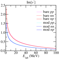
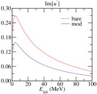
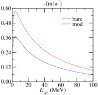
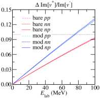
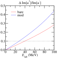
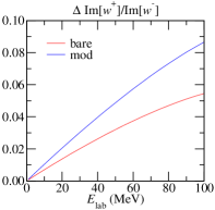
Figure 2: Top panels: the energy dependences of the $x^{-}$ type $S$–$P$ amplitudes. Bottom panels: the percentage deviations of $x^{+}/x^{-}$ from their zero-energy values $x^{+}(0)/x^{-}(0)$, where the dotted lines mark the $10\%$ level. 

The top panels of Fig. 2 show the energy dependences of $x^{-}$ ($x\in v_{pp,nn,np},\,u,\,w$) type $S$–$P$ amplitudes, proportional to $\langle\bm{y}_{m-}\rangle$, up to $E_{\mathrm{lab}}=100\,\mbox{MeV}$. Because the form factors suppress the short-distance contributions, the results from the “mod” calculations are consistently smaller than the “bare” ones. Another noticeable feature is the plots of $v_{pp}$, $v_{nn}$, and $v_{np}$ overlap, and the tiny difference is mostly due to the small charge-dependent interaction built in AV18.

The bottom panels of Fig. 2 show the percentage deviations of $x^{+}/x^{-}$ from their zero-energy values $x^{+}(0)/x^{-}(0)$, i.e.,

$$\Delta\,x^{+}/x^{-}\equiv\frac{x^{+}/x^{-}-x^{+}(0)/x^{-}(0)}{x^{+}(0)/x^{-}(0)}\,.$$ (21)

In case the energy dependences of $x^{+}$ and $x^{-}$ keep the same, $\Delta\,x^{+}/x^{-}$ remains zero. Therefore, this quantity is a measure of the departure from the perfect scaling, Eq. (19), which a strict 10-to-5 reduction scheme requires. As these plots show, the deviations all grow with energy in the positive direction. For the $v$ and $w$ amplitudes, the scaling actually works very well—though not perfect—up to $E_{\mathrm{lab}}=100\,\mbox{MeV}$ where the deviations are still less than $10\%$ for the “bare” case. For the $u$ amplitude, however, the $10\%$ tolerance for scaling deviation can only allow $E_{\mathrm{lab}}$ go as high as $40\,\mbox{MeV}$. It might come as a surprise why the $u$ and $w$ amplitudes have such different behaviors, since both involve the same ${}^{3}S_{1}$ wave and the ${}^{1}P_{1}$ wave (for $u$) does not differ from the ${}^{3}P_{1}$ one (for $w$) dramatically. The answer is due to the tensor force, by which a true distorted ${}^{3}S_{1}$-wave acquires some $D$-wave component. From the ratios

$$\langle^{1}P_{1}|\bm{\sigma}_{-}\cdot\hat{r}|^{3}S_{1},L=2\rangle/\langle^{1}P_{1}|\bm{\sigma}_{-}\cdot\hat{r}|^{3}S_{1},L=0\rangle =-\sqrt{2}\,,$$ (22)

$$\langle^{3}P_{1}|\bm{\sigma}_{+}\cdot\hat{r}|^{3}S_{1},L=2\rangle/\langle^{3}P_{1}|\bm{\sigma}_{+}\cdot\hat{r}|^{3}S_{1},L=0\rangle =1/\sqrt{2}\,,$$ (23)

one learns that the $D$-wave component is more enhanced in the $u$ than the $w$ amplitude, and this is the main cause of the difference. A mock calculation by pretending the ratio in Eq. (22) to be $1/\sqrt{2}$ as in Eq. (23) verifies that the scaling of $u^{+}/u^{-}$ would then be similar to $w^{+}/w^{-}$. The “mod” calculations generally show larger deviations, so the ranges within which the scalings work have to be reduced. This can be understood from that the difference of $\bm{y}_{m+}$ and $\bm{y}_{m-}$ is a term involving the gradient on the wave function. As the form factors suppress the short-range contribution, the longer-range part of the wave function which has a larger gradient thus gets a bigger weight; this leads to an enhancement of the deviation.

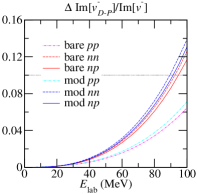
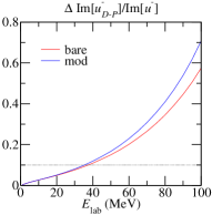
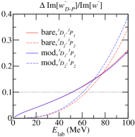
Figure 3: The percentage corrections induced by the $D$–$P$ transitions to the $S$–$P$ ones for the $x^{-}$ type amplitudes, where the dotted lines mark the $10\%$ level. 

The importance of the $D$–$P$ transitions is illustrated in Fig. 3, where their percentage corrections to the $S$–$P$ transitions are shown for the $x^{-}$ type amplitudes. Given a $10\%$ tolerance for corrections, one can conclude that the $S$–$P$ transitions dominate up to $E_{\mathrm{lab}}=90\,\mbox{MeV}$ for the $v$ type amplitudes (it can be higher for the $p\,p$ case because of the Coulomb repulsion) and up to $E_{\mathrm{lab}}=40\,\mbox{MeV}$ for both the $u$ and the $w$ types (note that the $w$ type contains two contributions from ${}^{3}D_{1}$–${}^{3}P_{1}$ and ${}^{3}D_{2}$–${}^{3}P_{2}$). The “mod” calculations do not change these conclusions too much. It should be stressed that these $D$–$P$ amplitudes have quite different energy dependences compared to the $S$–$P$ ones. Therefore, although the scaling behaviors found above for the $S$–$P$ amplitudes can apply to higher energies, the 10-to-5 reduction should be limited by the prerequisite of the $S$–$P$ dominance.

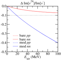
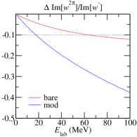
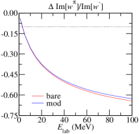
Figure 4: The percentage deviations of $x^{\pi,2\pi}/x^{-}$ from their zero-energy values $x^{\pi,2\pi}(0)/x^{-}(0)$, where the dotted lines mark the $10\%$ level. 

In Fig. 4, whether the OPE and TPE contributions can be effectively integrated out and lead to a purely pionless short-range potential is studied by examining the scaling behaviors of one- and two-pion amplitudes $x^{\pi,2\pi}$ with respect to $x^{-}$. As one can see, all the deviations increase with energy in the negative direction. In the “bare” calculations, the TPE amplitudes scale very well with the SR one. Allowing a $10\%$ deviation, the scaling works as $E_{\mathrm{lab}}$ reaches up to more than $100\,\mbox{MeV}$ for the $v$ amplitudes and $60\,\mbox{MeV}$ for the $w$ one; both limits are above the $S$–$P$-dominant region. On the other hand, the scaling works quite poorly—only up to $E_{\mathrm{lab}}=20\,\mbox{MeV}$—in the “mod” calculations. This can be easily seen from Fig. 1, where the modified two-pion Yukawa-like functions differs substantially from the bare ones at short distances. Since we have already mentioned the inconsistency of adding form factors to the TPE potential in such an ad hoc fashion in EFT, the curves labeled by “mod” for the TPE part should not be taken too seriously.

The most noteworthy information in Fig. 4 comes from the observation that it is almost impossible for the OPE amplitude to scale with the SR one, even within a modest energy range, say $10\,\mbox{MeV}$ or so. From threshold to $40\,\mbox{MeV}$, in which the $S$–$P$ dominance holds for the $w$ amplitude, the scaling deviation increases to $50\%$. Thus, this re-confirms the old wisdom that it takes two parameters—one for the SR and the other for the LR terms—to characterize the physics of the ${}^{3}S_{1}$–${}^{3}P_{1}$ transition Adelberger and Haxton (1985). In this sense, the applicability of the pionless EFT to nuclear PV is extremely limited, only within a very narrow energy range near threshold.

One might be temped to think that, as this bad scaling is due to the huge difference between the Yukawa mass scales: $m_{\mathrm{SR}}=m_{\rho}$ in $V_{1,\mathrm{SR}}^{\mathrm{PV}}$ and $m_{\mathrm{LR}}=m_{\pi}$ in $V_{-1,\mathrm{LR}}^{\mathrm{PV}}$, then, choosing a smaller mass scale in $V_{1,\mathrm{SR}}^{\mathrm{PV}}$ should make the pionless EFT work. The most straightforward choice is $m_{\mathrm{SR}}=m_{\pi}$—as long as the energy being considered is much smaller than $m_{\pi}$—by which the $w^{-}$ and $w^{\pi}$ amplitudes become identical. In this case, as Fig. 5 shows (the “mod” calculations are very close the the “bare” ones since the form factors do not cutoff the LR interaction too much), the scaling between $x^{+}$ and $x^{-}$ becomes extremely bad, and this completely spoils the nice reduction scheme of 10-to-5 LECs. For the $v$ and $w$ amplitudes, the $10\%$ scaling deviation only allows $E_{\mathrm{lab}}\lesssim 5\,\mbox{MeV}$; for the $u$ amplitude, it is even worse (the divergence at $E_{\mathrm{lab}}\sim 50\mbox{--}60\,\mbox{MeV}$ is because Im[$u^{-}$] crosses over the zero value). The reason is again that, by making the effective range of $V_{1,\mathrm{SR}}^{\mathrm{PV}}$ longer, the difference between $\langle\bm{y}_{m+}\rangle$ and $\langle\bm{y}_{m-}\rangle$ gets enhanced as the long-range part of the wave function, having a larger gradient, gets a bigger weight. Therefore, the price to pay for making the pionless EFT work is to keep all the 10 LECs as independent parameters. Clearly, the more economic choice would be keeping the OPE part explicitly and having the 10-to-5 reduction work by choosing $m_{\mathrm{SR}}=m_{\rho}$ for $V_{1,\mathrm{SR}}^{\mathrm{PV}}$.

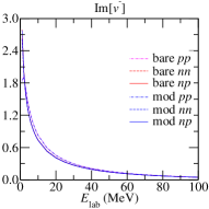
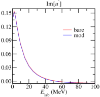
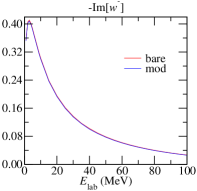
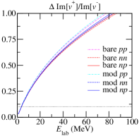
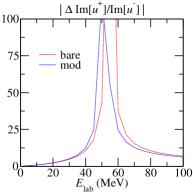
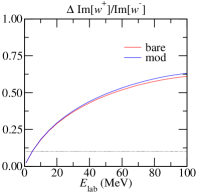
Figure 5: The similar analysis as Fig. 2 for the $x^{-}$ and $x^{+}$ amplitudes with the Yukawa mass parameter in $V_{-1,\mathrm{SR}}^{\mathrm{PV}}$ chosen to be $m=m_{\pi}$. The dotted line marks the $10\%$ level and it is not visible for the central bottom panel. 

To summarize the discussions so far, we conclude that at low energy, i.e., $E_{\mathrm{lab}}\lesssim 90\,\mbox{MeV}$ for ${}^{1}S_{0}$–${}^{3}P_{0}$ transitions and $E_{\mathrm{lab}}\lesssim 40\,\mbox{MeV}$ for ${}^{3}S_{1}$–${}^{1}P_{1}$ and ${}^{3}S_{1}$–${}^{3}P_{1}$ transitions, an PV potential formulated in EFT requires at least 6 parameters: 5 LECs plus $\widetilde{C}_{6}^{\pi}\propto h_{\pi}^{1}$. One may think that this conclusion makes $V_{\mathrm{EFT}}^{\mathrm{PV}}$ equivalent to $V_{\mathrm{OME}}^{\mathrm{PV}}$, which also has six PV parameters: 5 heavy-meson-nucleon couplings (ignoring $h_{\rho}^{1^{\prime}}$) plus $h_{\pi}^{1}$. However, this statement is not true in general, because the six-parameter EFT framework only works under the assumption of the $S$–$P$ dominance, but the OME framework is not limited by this requirement. Furthermore, the OME framework implies some prescribed relationships, Eqs. (9a, 9b, 10a, and 10b), between $C$’s and $\widetilde{C}$’s in the EFT framework; unfortunately, these relationships can not be justified without going to high energy.

At last, we come to the determination of the Danilov parameters, $\lambda_{s}^{pp,nn,np}$, $\lambda_{t}$, and $\rho_{t}$, which will serve as the 5 independent LECs. The relations between Danilov parameters and the zero-energy $S$–$P$ amplitudes are given by

$$v^{NN^{\prime}}(0) \approx-a_{s}^{NN^{\prime}}\,\mbox{e}^{i\,(\delta_{3P0}^{NN^{\prime}}(0)+\delta_{1S0}^{NN^{\prime}}(0))}\,\lambda_{s}^{NN^{\prime}}\,,$$ (24a)

$$u(0) \approx-a_{t}\,\mbox{e}^{i\,(\delta_{1P1}(0)+\delta_{3S1}(0))}\,\lambda_{t}\,,$$ (24b)

$$w_{\mathrm{SR}}(0) \approx-a_{t}\,\mbox{e}^{i\,(\delta_{3P1}(0)+\delta_{3S1}(0))}\,\rho_{t}\,,$$ (24c)

where $a$ denotes the corresponding scattering length and $\delta(0)$ the zero-energy phase shift (including the Coulomb contribution) Desplanques and Missimer (1978). The notation “$w_{\mathrm{SR}}$” means the OPE-subtracted ${}^{3}S_{1}$–${}^{3}P_{1}$ amplitude. Using the values $a_{s}^{pp}=-7.8064\,\mbox{fm}$, $a_{s}^{nn}=-18.487\,\mbox{fm}$, $a_{s}^{np}=-23.7318\,\mbox{fm}$, and $a_{t}=5.4192\,\mbox{fm}$, we get the dimensionless Danilov parameters

$$m_{\scriptscriptstyle{N}}\lambda_{s}^{pp} =5.507\times 10^{-3}\,(\widetilde{D}_{v}^{pp}+0.789\,D_{v}^{pp}-1.655\,\widetilde{C}_{2}^{2\pi})\,,$$ (25a)

$$m_{\scriptscriptstyle{N}}\lambda_{s}^{nn} =5.796\times 10^{-3}\,(\widetilde{D}_{v}^{nn}+0.792\,D_{v}^{nn}-1.648\,\widetilde{C}_{2}^{2\pi})\,,$$ (25b)

$$m_{\scriptscriptstyle{N}}\lambda_{s}^{np} =5.778\times 10^{-3}\,(\widetilde{D}_{v}^{np}+0.809\,D_{v}^{np})\,,$$ (25c)

$$m_{\scriptscriptstyle{N}}\lambda_{t} =-1.462\times 10^{-3}\,(\widetilde{D}_{u}-2.230\,D_{u})\,,$$ (25d)

$$m_{\scriptscriptstyle{N}}\rho_{t} =3.108\times 10^{-3}\,(\widetilde{D}_{w}+0.604\,D_{w}-1.771\,\widetilde{C}_{6}^{2\pi})\,;$$ (25e)

for the “bare” case; and

$$m_{\scriptscriptstyle{N}}\bar{\lambda}_{s}^{pp} =3.268\times 10^{-3}\,(\widetilde{D}_{v}^{pp}+0.849\,D_{v}^{pp}-1.260\,\widetilde{C}_{2}^{2\pi})\,,$$ (26a)

$$m_{\scriptscriptstyle{N}}\bar{\lambda}_{s}^{nn} =3.809\times 10^{-3}\,(\widetilde{D}_{v}^{nn}+0.853\,D_{v}^{nn}-1.237\,\widetilde{C}_{2}^{2\pi})\,,$$ (26b)

$$m_{\scriptscriptstyle{N}}\bar{\lambda}_{s}^{np} =3.772\times 10^{-3}\,(\widetilde{D}_{v}^{np}+0.871\,D_{v}^{np})\,,$$ (26c)

$$m_{\scriptscriptstyle{N}}\bar{\lambda}_{t} =-0.867\times 10^{-3}\,(\widetilde{D}_{u}-2.425\,D_{u})\,,$$ (26d)

$$m_{\scriptscriptstyle{N}}\bar{\rho}_{t} =2.003\times 10^{-3}\,(\widetilde{D}_{w}+0.664\,D_{w}-1.586\,\widetilde{C}_{6}^{2\pi})\,,$$ (26e)

for the “mod” case.

In these expressions, one sees that the scaling factors between $D$’s and $\widetilde{D}$’s are not $1$ as anticipated by the ZRA with the absence of hard core. The most striking case, which amounts to $2.230$ (or $2.425$ for the “mod” case), happens for the ${}^{1}P_{1}$–${}^{3}S_{1}$ transition. This in fact shows the attractiveness of the hybrid EFT treatment for nuclear PV: one gets the strong dynamics right without having to go to a higher order in $Q$, where the proliferation of needed PV parameters is totally undesirable.

IV Parity-Violating Observables in Two-Nucleon Systems 

Having determined a minimal set of PV parameters, i.e., $m_{\scriptscriptstyle{N}}\lambda_{s}^{pp,nn,np}$, $m_{\scriptscriptstyle{N}}\lambda_{t}$, $m_{\scriptscriptstyle{N}}\rho_{t}$ and $\widetilde{C}_{6}^{\pi}$, to describe the low-energy PV phenomena, we will use them in this section to express the PV observables which have been or will be measured in two-body systems. As analyses of these observables have been quite extensively discussed in the $V_{\textrm{OME}}^{\textrm{PV}}$ framework, we refer most of the details which also apply to the EFT framework to literature and only highlight the new results and the comparison with the old framework.

IV.1 $A_{L}^{\vec{p}p}$ in $\vec{p}\,p$ scattering

The “nuclear” total asymmetry for $\vec{p}\,p$ scattering Simonius (1972, 1974, 1988); Nessi-Tedaldi and Simonius (1988); Driscoll and Miller (1989); Carlson et al. (2002),

$$A_{L}^{\vec{p}p}(E)=\frac{\textrm{Im}\left[\widetilde{\mathcal{M}}_{10,00}(E,0)+\widetilde{\mathcal{M}}_{00,10}(E,0)\right]}{\textrm{Im}\left[{\displaystyle{\sum_{S,M_{S}}}}\mathcal{M}_{SM_{S},SM_{S}}(E,0)\right]}\,,$$ (27)

is defined through the Coulomb-subtracted, forward ($\theta=0$) scattering amplitude $\mathcal{M}(E,0)$, where the subscript pair $S^{\prime}M^{\prime}_{S},SM_{S}$ denotes the final and initial two-body spin states, respectively. As the Coulomb scattering amplitude, $M^{\textrm{C}}$, diverges at the forward angle, the total asymmetry (with full $4\,\pi$ angular coverage) can only be well-defined after this singular piece is subtracted: $\mathcal{M}\equiv M-M^{\textrm{C}}$. One should note that $A_{L}^{\vec{p}p}$ is not a quantity an experiment directly measures; a theoretical correction is needed to fold an experimental result into $A_{L}^{\vec{p}p}(E)$ (see, e.g., Refs. Driscoll and Miller (1989); Carlson et al. (2002) for more discussions).

Currently, there are two low-energy data points at $13.6\,\textrm{MeV}$ and $45\,\textrm{MeV}$ which give $A_{L}^{\vec{p}p}=-(0.93\pm 0.21)\times 10^{-7}$ Eversheim et al. (1991); Haeberli and Holstein (1995) and $-(1.57\pm 0.23)\times 10^{-7}$ Kistryn et al. (1987), respectively. These supersede the earlier, less accurate experiments at $15$ and $45\,\textrm{MeV}$ which yield $-(1.7\pm 0.8)\times 10^{-7}$ Potter et al. (1974); Nagle et al. (1979) and $-(2.31\pm 0.89)\times 10^{-7}$ Balzer et al. (1980, 1984), respectively. At higher energy, there is one measurement at $221\,\textrm{MeV}$, yielding $+(0.84\pm 0.29)\times 10^{-7}$ Berdoz et al. (2001, 2003); it is motivated by the theoretical prediction that this would uniquely determine the PV $\rho$-exchange coupling constant $h_{\rho}^{pp}\equiv h_{\rho}^{0}+h_{\rho}^{1}+h_{\rho}^{2}/\sqrt{6}$ in $V_{\textrm{OME}}^{\textrm{PV}}$ Simonius (1988).

Table 3: Analysis of $A_{L}^{\vec{p}p}$ decomposed in partial waves. Each entry denotes the multiplicative coefficient for the corresponding PV coupling constant. The full result is the sum of every “entry$\times$coupling” in the same row. The last column “OME-m” shows the numerical value of $A_{L}^{\vec{p}p}$ by performing the OME-mapping to the EFT result with the PC and PV parameters specified in Tabs. 1 and 2. 

		${}^{1}S_{0}\textrm{--}^{3}P_{0}\,(\times 10^{-3})$			${}^{1}D_{2}\textrm{--}^{3}P_{2}\,(\times 10^{-3})$			${}^{1}D_{2}\textrm{--}^{3}F_{2}\,(\times 10^{-3})$			OME-m
		$D_{v}^{pp}$	$\widetilde{D}_{v}^{pp}$	$\widetilde{C}_{2}^{2\pi}$	$D_{v}^{pp}$	$\widetilde{D}_{v}^{pp}$	$\widetilde{C}_{2}^{2\pi}$	$D_{v}^{pp}$	$\widetilde{D}_{v}^{pp}$	$\widetilde{C}_{2}^{2\pi}$	$(\times 10^{-7})$
$13.6$	bare	$-1.980$	$-2.476$	$4.010$	$-0.005$	$0.006$	$-0.012$	$0.001$	$-0.001$	$0.002$	$-0.971$
	mod	$-1.398$	$-1.617$	$1.885$	$-0.004$	$0.004$	$-0.010$	$0.000$	$-0.001$	$0.001$	$-0.960$
$45$	bare	$-3.686$	$-4.476$	$7.026$	$-0.122$	$0.132$	$-0.243$	$0.027$	$-0.033$	$0.064$	$-1.746$
	mod	$-2.582$	$-2.868$	$2.842$	$-0.089$	$0.094$	$-0.180$	$0.019$	$-0.023$	$0.050$	$-1.662$
$221$	bare	$-0.069$	$-0.073$	$0.112$	$-2.749$	$2.618$	$-3.784$	$0.164$	$-0.388$	$0.633$	$0.426$
	mod	$-0.046$	$-0.043$	$0.015$	$-1.888$	$1.678$	$-1.636$	$0.086$	$-0.270$	$0.420$	$0.853$

The EFT analysis of $A_{L}^{\vec{p}p}$ for the low-energy data points is tabulated in Tab. 4. Apparently, the observables are dominated by the $S$–$P$ transition. Using the Danilov parameters obtained in the last section, we find that

$$A_{L}^{\vec{p}p}(13.6\,\mbox{MeV}) =-0.449\,m_{\scriptscriptstyle{N}}\lambda_{s}^{pp}+(-0.035\,D_{v}^{pp}-0.088\,\widetilde{C}_{2}^{2\pi})\times 10^{-3}\quad(\mbox{bare}),$$

$$\mbox{or}-0.445\,m_{\scriptscriptstyle{N}}\bar{\lambda}_{s}^{pp}+(-0.032\,D_{v}^{pp}-0.157\,\widetilde{C}_{2}^{2\pi})\times 10^{-3}\quad(\mbox{mod});$$ (28)

$$A_{L}^{\vec{p}p}(45\,\mbox{MeV}) =-0.795\,m_{\scriptscriptstyle{N}}\lambda_{s}^{pp}+(-0.329\,D_{v}^{pp}-0.395\,\widetilde{C}_{2}^{2\pi})\times 10^{-3}\quad(\mbox{bare}),$$

$$\mbox{or}-0.771\,m_{\scriptscriptstyle{N}}\bar{\lambda}_{s}^{pp}+(-0.276\,D_{v}^{pp}-0.813\,\widetilde{C}_{2}^{2\pi})\times 10^{-3}\quad(\mbox{mod}).$$ (29)

The correction terms, enclosed in parentheses, are in general quite small except for the TPE parts in the “mod” calculations, so we conclude that these two data only depend on one single parameter, $m_{\scriptscriptstyle{N}}\lambda_{s}^{pp}$. In fact, the theoretical prediction for the ratio of $A_{L}^{\vec{p}p}(45\,\mbox{MeV})/A_{L}^{\vec{p}p}(13.6\,\mbox{MeV})\approx-0.795/-0.449=1.77$ (or $-0.771/-0.445=1.73$ for the “mod” case) agrees very well with the experimental result $\approx-1.57/-0.93=1.69$ (discarding errors). Furthermore, one can see from the comparison between the “bare” and “mod” results that even though $m_{\scriptscriptstyle{N}}\lambda_{s}^{pp}$ and $m_{\scriptscriptstyle{N}}\bar{\lambda}_{s}^{pp}$ are defined in different models, the expressions for $A_{L}^{\vec{p}p}$ in terms of them are almost model-independent. This justifies the advantage of using the Danilov parameters instead of the LECs $C$’s, $\widetilde{C}^{\prime}s$, etc.

Even though it is doubtful that the $V_{\mathrm{EFT}}^{\textrm{PV}}$ of order $O(Q)$ is sufficient for analyzing the high-energy datum at $221\,\textrm{MeV}$, it is nonetheless interesting to see how the analysis turns out to be. The result, also shown in Tab. 4, indicates a quite different feature. The $D\textrm{--}P$ amplitude becomes the most dominant contribution, with the $D$–$F$ one also being non-negligible. Both amplitudes have their own scaling factors between $D_{v}^{pp}$, $\widetilde{D}_{v}^{pp}$, and $\widetilde{C}_{2}^{2\pi}$ components different from the $S$–$P$ amplitude. While it is not clear if the $D$–$P$ and $D$–$F$ amplitudes can be completely specified by $D_{v}^{pp}$, $\widetilde{D}_{v}^{pp}$, and $\widetilde{C}_{2}^{2\pi}$, they certainly can not be uniquely fixed by the only high-energy measurement.

By OME-mapping the EFT results in Tab. 4, our calculations are checked with literature. The “bare+DDH-best” results are consistent with works such as Refs. Simonius (1972, 1974, 1988); Nessi-Tedaldi and Simonius (1988), given that different strong potential models are used. The “mod+DDH-adj.” results agree well with Refs. Driscoll and Miller (1989); Carlson et al. (2002); the small difference is because we do not use a different mass and a cutoff factor for the $\omega$ meson.

It is worth to point out that the analysis by Carlson et al. Carlson et al. (2002), which is based on a OME framework with two independent parameters $h_{\rho}^{pp}$ and $h_{\omega}^{pp}$, claims a good fit to both low- and high-energy data. Unfortunately, due to the lack of more high energy data, it is currently impossible to verify this fit along with its important dynamical assumptions—the monopole form factors and big isovector tensor coupling $\chi_{\rho}$—within the EFT framework. On the other hand, their fitted PV $\omega NN$ coupling constant, $h_{\omega}^{pp}=h_{\omega}^{0}+h_{\omega}^{1}$, is only marginally consistent with most hadronic perditions and needs further clarification. For these issues, we refer to Ref. Liu et al. (2006) for more discussions.

Finally, we turn our attention to the TPE contributions, which have not received extensive study and are left out while we do the OME-mapping in Tab. 4. By writing out $\widetilde{C}_{2}^{2\pi}$ in term of $h_{\pi}^{1}$ explicitly and assuming the DDH best value for $h_{\pi}^{1}$, one sees the asymmetry in the “bare” case increased by $\sim 70\%$ for the $13.6$ and $45\,\mbox{MeV}$ data points and $\sim 60\%$ for the $221\,\mbox{MeV}$ one. In the “mod” case, the increases are $\sim 30\%$ and $\sim 20\%$ for low- and high-energy cases, respectively. Although these corrections seem quite big, one should remember they are not the full TPE corrections, as part of the TPE contributions are buried in the SR interaction. But since $V_{1,\mathrm{MR}}^{\mathrm{PV}}$ and $V_{1,\mathrm{SR}}^{\mathrm{PV}}$ have the same power counting, it is not unnatural to expect individual terms of similar magnitude. Another remark concerns the general trends that the TPE enhances the asymmetry and it is the the low-energy cases that get more boost than the high-energy ones. These points have also been noticed in Ref. Liu et al. (2006), where part of the TPE contribution is accounted for by formulating it as a $\rho$-resonance.

IV.2 $\phi_{n}^{\vec{n}p}$ and $P_{n}^{np}$ in neutron transmission through para-hydrogen

It was first pointed by Michel Michel (1964) and later on by Stodolsky Stodolsky (1974, 1982) that nuclear parity violation can be studied through low-energy neutron transmission, where the whole process acts like optics. The observables could be a spin rotation, $\phi_{n}$, about the longitudinal axis (assumed to be $\hat{z}$) for the transversely-polarized neutron, or a net longitudinal polarization, $P_{n}$, that an unpolarized neutron beam picks up when traversing through medium—the latter is equivalent to the asymmetry in cross section for the longitudinally-polarized neutron scattering, $A_{L}^{\vec{n}p}$. These quantities per unit length (assuming the target is uniform), $d\,\phi_{n}/d\,z$ and $d\,P_{n}/d\,z$, can be related to the PV forward scattering amplitude $\widetilde{M}(E,0)$ by

$$\frac{d\,\phi_{n}}{d\,z} =-\frac{2\,\pi}{k}\,N\,\textrm{Re}(\widetilde{M}_{+z}(E,0)-\widetilde{M}_{-z}(E,0))\,,$$ (30)

$$\frac{d\,P_{n}}{d\,z} =-\frac{2\,\pi}{k}\,N\,\textrm{Im}(\widetilde{M}_{+z}(E,0)-\widetilde{M}_{-z}(E,0))\,,$$ (31)

where $k$ is the magnitude of the neutron momentum, $N$ is the target number density, and the subscript $\pm z$ denotes the direction of neutron polarization.

For a thermal neutron beam, $E_{n}\approx 0.025\,\textrm{eV}$, transmitting through liquid para-hydrogen, $N=0.24\times 10^{23}/\textrm{cm}^{3}$, the EFT analysis of $d\,\phi_{n}/d\,z$ and $d\,P_{n}/d\,z$ is tabulated in Tab. 5. At thermal energy, the magnitude of $d\,P_{n}^{np}/d\,z$ is about four orders of magnitude smaller than $d\,\phi_{n}^{\vec{n}p}/d\,z$. When neutron energy is further decreased, $d\,\phi_{n}^{\vec{n}p}/d\,z$ stays constant, but $d\,P_{n}^{np}/d\,z$ drops as $\sqrt{E_{n}}$; therefore, the spin-rotation measurement is more feasible for low-energy neutrons. This trend is consistent with the argument made by Stodolsky Stodolsky (1982) about the elastic scattering. It is also pointed out in Ref. Stodolsky (1982) that exothermic processes, i.e., inelastic exit channels, can possibly result in a non-vanishing $d\,P_{n}/d\,z$ at zero energy. However, it is not the case for $n\,p$ scattering, where the only exothermic reaction, $n\,p\rightarrow d\,\gamma$ (will be discussed in Sec. IV.4), does not lead to a total asymmetry, as remarked in Ref. Liu and Timmermans (2006).

Table 5: Analysis of (I) $d\,\phi_{n}^{\vec{n}p}(\textrm{th.})/d\,z$ in rad/m and (II) $d\,P_{n}^{np}(\textrm{th.})/d\,z$ in $10^{-4}/\textrm{m}$ decomposed in partial waves. See Tab.  4 for the explanation of tabularization. 

		${}^{1}S_{0}\textrm{--}^{3}P_{0}\,(\times 10^{-2})$		${}^{3}S_{1}\textrm{--}^{1}P_{1}\,(\times 10^{-2})$		${}^{3}S_{1}\textrm{--}^{3}P_{1}\,(\times 10^{-2})$				OME-m
		$D_{v}^{np}$	$\widetilde{D}_{v}^{np}$	$D_{u}$	$\widetilde{D}_{u}$	$D_{w}$	$\widetilde{D}_{w}$	$\widetilde{C}_{6}^{\pi}$	$\widetilde{C}_{6}^{2\pi}$	$(\times 10^{-7})$
(I)	bare	$1.169$	$1.444$	$-0.186$	$0.083$	$0.214$	$0.355$	$0.286$	$-0.628$	$6.711$
	mod	$0.821$	$0.943$	$-0.120$	$0.049$	$0.152$	$0.229$	$0.284$	$-0.363$	$5.149$
(II)	bare	$4.805$	$5.939$	$0.175$	$-0.079$	$-0.202$	$-0.334$	$-0.269$	$0.591$	$2.165$
	mod	$3.378$	$3.878$	$0.113$	$-0.047$	$-0.143$	$-0.215$	$-0.267$	$0.341$	$-2.220$

In this case, all three different $S\textrm{--}P$ amplitudes come into play, and the results in terms of Danilov parameters and $\widetilde{C}_{6}^{\pi}$ are

$$\frac{d\,\phi_{n}^{\vec{n}p}(\mathrm{th.})}{d\,z}\Big{|}_{\mathrm{m/rad}} =0.286\,\widetilde{C}_{6}^{\pi}+2.500\,m_{\scriptscriptstyle{N}}\lambda_{s}^{np}-0.571\,m_{\scriptscriptstyle{N}}\lambda_{t}+1.412\,m_{\scriptscriptstyle{N}}\rho_{t}+(0.000)\quad(\mbox{bare});$$

$$\mbox{or }0.284\,\widetilde{C}_{6}^{\pi}+2.500\,m_{\scriptscriptstyle{N}}\bar{\lambda}_{s}^{np}-0.571\,m_{\scriptscriptstyle{N}}\bar{\lambda}_{t}+1.412\,m_{\scriptscriptstyle{N}}\bar{\rho}_{t}+(0.000)\quad(\mbox{mod}).$$ (32)

Because this process is close to zero energy, it is not a surprise that the Danilov parameters work extremely well (almost no error). Also, this expression is model-independent, no matter it is for the “bare” or the “mod” calculation.

By OME-mapping the EFT results, the “bare+DDH-best” value, $d\,\phi_{n}^{\vec{n}p}(\textrm{th.})/d\,z\simeq 6.71\times 10^{-7}\,\textrm{rad}/\textrm{m}$, is about $20\%$ smaller in magnitude than an early prediction using the Paris potential Avishai and Grange (1984), and with a different sign. Thus, we confirm the assertion of Ref. Schiavilla et al. (2004) about the sign problem in Ref. Avishai and Grange (1984). As for the “mod+DDH-adj” value, $\simeq 5.15\times 10^{-7}\,\textrm{rad}/\textrm{m}$, it agrees well with Ref. Schiavilla et al. (2004). If these numerical estimates are not too far off, the plan of doing such an experiment aiming at a $2.7\times 10^{-7}\,\textrm{rad/m}$ precision Markov (2002) at the Spallation Neutron Source (SNS) will certainly provide a valuable data point.

The TPE contribution enters through the ${}^{3}S_{1}$–${}^{3}P_{1}$ transition. Because $\widetilde{C}_{6}^{\pi}$ and $\widetilde{C}_{6}^{2\pi}$ have the same sign, Tab. 5 suggests that the TPE reduces the OPE contribution which dominates the above OME-m estimates. The correction is about $-15\%$ for the “bare” calculation, and $-10\%$ for the “mod” calculation. This $\sim 10\%$ correction is consistent with the qualitative power-counting argument that the TPE contribution is smaller than the leading OPE one by an order of magnitude.

IV.3 $P_{\gamma}^{np}$ in $n\,p\rightarrow d\,\gamma$ and $A_{L}^{\vec{\gamma}d}$ in $\vec{\gamma}\,d\rightarrow n\,p$ 

Low-energy radiative neutron capture mainly involves the lowest-order electromagnetic transitions. For $n\,p\rightarrow d\,\gamma$, it is $M1$ for the PC part, and $E1$ for the PV part. Since the total cross section is dominated by the ${}^{1}S_{0}$-wave scattering, the non-zero circular polarization takes an approximate simple form as

$$P_{\gamma}^{np}=2\,\frac{\bra{\mathcal{D}}|E_{1}|\widetilde{\ket{{}^{3}P_{0}}}+\vspace{0.5cm}_{\mathcal{D}}\widetilde{\bra{{}^{1}P_{1}}}|E_{1}|\ket{{}^{1}S_{0}}}{\bra{\mathcal{D}}|M_{1}|\ket{{}^{1}S_{0}}}\,,$$ (33)

where the double bar “$||$” denotes the reduced matrix element. In this case, the observable depends on the ${}^{1}S_{0}\textrm{--}^{3}P_{0}$ and the deuteron $\mathcal{D}\textrm{--}^{1}P_{1}$ admixtures. It is important to recognize that we rely on the Siegert theorem Siegert (1937), through which the $E_{1}$ operator is related to the charge dipole operator $C_{1}$, to calculate the $E1$ matrix elements. This manipulation not only implicitly includes most $\mathcal{O}(v/c)$ meson exchange currents, but also imposes a $\Delta S=0$ spin selection rule as shown in Eq. (33).

Table 6: Analysis of $P_{\gamma}^{np}(\textrm{th.})$ decomposed in partial waves. See Tab.  4 for the explanation of tabularization. 

	${}^{1}S_{0}\textrm{--}^{3}P_{0}$ mix. $(\times 10^{-3})$		$\mathcal{D}\textrm{--}^{1}P_{1}$ mix. $(\times 10^{-3})$		OME-m
	$D_{v}^{np}$	$\widetilde{D}_{v}^{np}$	$D_{u}$	$\widetilde{D}_{u}$	$(\times 10^{-7})$
bare	$-0.751$	$-0.935$	$2.166$	$-0.980$	$0.247$
mono	$-0.525$	$-0.607$	$1.391$	$-0.580$	$0.520$

For thermal neutron, the EFT analysis is tabulated in Tab. 6. Although the observable $P_{\gamma}^{np}$ is not determined directly by the scattering amplitudes—instead, by the parity admixtures which do not have a trivial relation to the scattering amplitudes in general—the Danilov parameters still do a good job

$$P_{\gamma}^{np}(\mbox{th.}) =-0.161\,m_{\scriptscriptstyle{N}}\lambda_{s}^{np}+0.670\,m_{\scriptscriptstyle{N}}\lambda_{t}+(0.005\,D_{v}^{np}+0.019\,D_{u})\times 10^{-3}\quad(\mbox{bare});$$

$$\mbox{or }-0.161\,m_{\scriptscriptstyle{N}}\bar{\lambda}_{s}^{np}+0.669\,m_{\scriptscriptstyle{N}}\bar{\lambda}_{t}+(0.004\,D_{v}^{np}+0.016\,D_{u})\times 10^{-3}\quad(\mbox{mod}).$$ (34)

The reason is mainly because the process occurs at a very low energy and the deuteron is a loosely bound state; both are not far from the zero-energy limit.

The OME-mapping gives the “bare+DDH-best” value $P_{\gamma}^{np}(\textrm{th.})=2.5\times 10^{-8}$ which agrees well with a recent calculation Hyun et al. (2005) and is also consistent with pre-80’s predictions, e.g., Refs. Tadic (1968); Danilov (1971); Lassey and McKellar (1975); Desplanques (1975); Craver et al. (1976), around $(2\textrm{--}5)\times 10^{-8}$, (see Ref. Lassey and McKellar (1976) for a summary). For the “mod+DDH-adj.” value $P_{\gamma}^{np}(\textrm{th.})=0.52\times 10^{-7}$, we have an excellent check with Ref. Schiavilla et al. (2004).

Historically, the first measurement of $P_{\gamma}^{np}(\textrm{th.})$ done by the Leningrad group reports a result $-(1.3\pm 0.45)\times 10^{-6}$ Lobashov et al. (1972), which not only exceeds most theoretical predictions by two orders of magnitude but also has an opposite sign. The follow-up experiment does correct the sign problem; however, the published result $P_{\gamma}^{np}(\textrm{th.})=(1.8\pm 1.8)\times 10^{-7}$ Knyaz’kov et al. (1984) still has too large an error bar. In order to circumvent the difficulty of measuring a circular polarization, the inverse process, the asymmetry $A_{L}^{\vec{\gamma}d}$ in deuteron photo-disintegration, $\vec{\gamma}\,d\rightarrow n\,p$, can be a good alternative. By detailed balancing, $A_{L}^{\vec{\gamma}d}=P_{\gamma}^{np}$ if all kinematics are exactly reversed. One can show that, for photon with energy of $1.32\,\textrm{keV}$ above the threshold, $A_{\gamma}^{\vec{\gamma}d}(1.32\,\textrm{keV}+)=P_{\gamma}^{np}(\textrm{th.})$.

As demonstrated in several theoretical works Lee (1978); Oka (1983); Fujiwara and Titov (2004); Liu et al. (2004); Schiavilla et al. (2004), the asymmetry $A_{L}^{\vec{\gamma}d}$ gets larger when approaching the threshold, but on the other hand, the total cross section gets smaller. There are two data points reported in 80s: $(2.7\pm 2.8)\times 10^{-6}$ at $E_{\gamma}=4.1\,\textrm{MeV}$ and $(7.7\pm 5.3)\times 10^{-6}$ at $E_{\gamma}=3.2\,\textrm{MeV}$ Earle et al. (1988); Alberi et al. (1988); though they qualitatively justify the statement above, the precisions are too low to be of use. With various groups showing interests of new measurements (e.g., Ref. Wojtsekhowski and van Oers ), it is important to decide the best photon energy (should not be too far from the threshold for larger asymmetry) to be employed.

An important point to note for this particular observable is that, unlike the case for neutron transmission, the $\mathcal{D}\textrm{--}^{1}P_{1}$ admixture has an important contribution so that the model dependence is worrisome. The situation is most clear when comparing with other semi- and non-local potential model calculations. As shown in Refs. Schiavilla et al. (2004); Hyun et al. (2005), the CD-Bonn and Bonn-B calculations give predictions two times larger, and the Bonn calculation even enhances by an order of magnitude. The difference is mostly due to the large variations of these models in the ${}^{1}P_{1}$ channel at short distances Hyun et al. (2005). In this sense, a well-determined $\lambda_{t}$, if ever possible, can be used in a reversed way to constrain strong potential models.

IV.4 $A_{\gamma}$ in $\vec{n}\,p\rightarrow d\,\gamma$ 

By the same approximation as in the above subsection, the photon asymmetry in $\vec{n}\,p\rightarrow d\,\gamma$, $A_{\gamma}^{\vec{n}p}$, which is defined through $d\,\sigma_{\pm}(\theta)/d\,\Omega\propto 1\pm A_{\gamma}^{\vec{n}p}\,\cos\theta$,  can be expressed as

$$A_{\gamma}^{\vec{n}p}=-\sqrt{2}\,\frac{\bra{\mathcal{D}}|E_{1}|\widetilde{\ket{{}^{3}P_{1}}}+\vspace{0.5cm}_{\mathcal{D}}\widetilde{\bra{{}^{3}P_{1}}}|E_{1}|\ket{{}^{3}S_{1}}}{\bra{\mathcal{D}}|M_{1}|\ket{{}^{1}S_{0}}}\,.$$ (35)

Unlike the case for $P_{\gamma}^{np}$, it is the ${}^{3}S_{1}\textrm{--}^{3}P_{1}$ and $\mathcal{D}\textrm{--}^{3}P_{1}$ admixtures that contribute in this case.

Table 7: Analysis of $A_{\gamma}^{\vec{n}p}(\textrm{th.})$ decomposed in partial waves. See Tab.  4 for the explanation of tabularization. 

	${}^{3}S_{1}\textrm{--}^{3}P_{1}$ mix. $(\times 10^{-3})$				$\mathcal{D}\textrm{--}^{3}P_{1}$ mix. $(\times 10^{-3})$				OME-m
	$D_{w}$	$\widetilde{D}_{w}$	$\widetilde{C}_{6}^{\pi}$	$\widetilde{C}_{6}^{2\pi}$	$D_{w}$	$\widetilde{D}_{w}$	$\widetilde{C}_{6}^{\pi}$	$\widetilde{C}_{6}^{2\pi}$	$(\times 10^{-7})$
bare	$-0.108$	$-0.185$	$-0.133$	$0.321$	$-0.066$	$-0.103$	$-0.139$	$0.193$	$-0.506$
mod	$-0.076$	$-0.118$	$-0.132$	$0.172$	$-0.048$	$-0.069$	$-0.138$	$0.128$	$-0.486$

For thermal neutron, the EFT analysis is tabulated in Tab. 7. Again, the Danilov parameter $m_{\scriptscriptstyle{N}}\rho_{t}$ pretty much summarizes the short-distance physics

$$A_{\gamma}^{\vec{n}p}(\textrm{th.}) =-0.272\,\widetilde{C}_{6}^{\pi}-0.093\,m_{\scriptscriptstyle{N}}\rho_{t}+(0.003\,\widetilde{C}_{6}^{2\pi})\times 10^{-3}\quad(\mbox{bare});$$

$$\mbox{or }-0.270\,\widetilde{C}_{6}^{\pi}-0.093\,m_{\scriptscriptstyle{N}}\bar{\rho}_{t}+(0.004\,\widetilde{C}_{6}^{2\pi})\times 10^{-3}\quad(\mbox{mod}).$$ (36)

The OME-mapping values, $A_{\gamma}^{\vec{n}p}(\textrm{th.})=-5.06\times 10^{-8}$ for the “bare+DDH-best” case and $-4.85\times 10^{-8}$ for the “bare+DDH-adj.” case, are consistent with existing predictions, e.g., Refs. Tadic (1968); Danilov (1971); Desplanques (1975); Lassey and McKellar (1976); Kaplan et al. (1999); Savage (2001); Desplanques (2001); Hyun et al. (2001, 2005) for the former and Refs. Schiavilla et al. (2003, 2004) for the latter, respectively.

The TPE contributions change the above OME-m results somewhat. Their corrections to the OPE contributions are $-13\%$ and $-8\%$ for the “bare” and “mod” cases, respectively. This is similar to the neutron spin rotation case, and consistent with a recent calculation Hyun et al. .

The great interest of measuring $A_{\gamma}^{\vec{n}p}$ is mainly because it is dominated by the OPE in the $V_{\textrm{OME}}^{\textrm{PV}}$ framework. This can also be observed from the above EFT analysis: If one assumes the natural size of $m_{\scriptscriptstyle{N}}\rho_{t}/\widetilde{C}_{6}^{\pi}\sim 0.1$, the OPE contribution then dominates the SR one by a factor of $30$ or so.  One of the outstanding puzzles in nuclear PV is the difficulty of accommodating the extremely small upper limit on $h_{\pi}^{1}$, set by the ${}^{18}\textrm{F}$ results Adelberger and Haxton (1985), with hadronic predictions and other nuclear PV experiments. The NPDGamma experiment Snow et al. (2000), currently running at the Los Alamos Neutron Science Center (LANSCE) and will be at SNS later on, aims to reach an ultimate sensitivity of $5\times 10^{-9}$. Results from this experiment will certainly improve the long-existing value: $(0.6\pm 2.1)\times 10^{-7}$ Cavaignac et al. (1977); Alberi et al. (1988), and hopefully resolve the $h_{\pi}^{1}$ puzzle.

Concluding this section, we shall make an important remark about the PV meson exchange current (MEC) effects which manifest in electromagnetic processes such as radiative neutron capture being discussed here and in Sec.  IV.3. Although the Siegert theorem alleviates much of the problem regarding the calculations of transverse electric multipole operators $E_{J}$’s due to MECs, there is no easy simplification when the transverse magnetic multipole operators $M_{J}$’s are concerned. Furthermore, the Siegert theorem only applies to MECs which are constrained by the continuity equation; for other transverse MECs, their effects to $E_{J}$’s have to be added separately.

In Ref. Zhu et al. (2005), there is indeed such a transverse MEC, which can not be accounted for by gauging the PV interaction, and it introduces a new PV constant designated as $\bar{c}_{\pi}$. This MEC takes the following form in the configuration space

$$\bm{j}_{\bar{c}_{\pi}}(\bm{x};\bm{x}_{1},\bm{x}_{2})= -i\,\frac{\sqrt{2}\,g_{\pi}\,\bar{c}_{\pi}}{m_{\scriptscriptstyle{N}}\,\Lambda_{\chi}\,F_{\pi}}\,(\tau_{1+}\,\tau_{2-})\left[\bm{\sigma}_{2}\cdot\hat{r}\,\bm{\sigma}_{1}\times\bm{\nabla}_{x}\,\delta^{(3)}(\bm{x}-\bm{x}_{1})\right]$$

$$\times\frac{\mbox{e}^{-m_{\pi}\,r}}{4\,\pi\,r^{2}}\,(1+m_{\pi}\,r)+(1\leftrightarrow 2)\,,$$ (37)

where $\tau_{\pm}=\tau_{x}\pm i\,\tau_{y}$, and $r=|\bm{x}_{1}-\bm{x}_{2}|$. Compared with the dominant part of the PV OPE MEC, the so-called pair current,

$$\bm{j}_{\pi\mathrm{pair}}(\bm{x};\bm{x}_{1},\bm{x}_{2})= -\frac{g_{\pi}\,h_{\pi}^{1}}{2\,\sqrt{2}\,m_{\scriptscriptstyle{N}}}\,(\bm{\tau}_{1}\cdot\bm{\tau}_{2}-\tau_{1}^{z}\,\tau_{2}^{z})\left[\bm{\sigma}_{1}\,\delta^{(3)}(\bm{x}-\bm{x}_{1})\right]$$

$$\times\frac{\mbox{e}^{-m_{\pi}\,r}}{4\,\pi\,r}+(1\leftrightarrow 2)\,,$$ (38)

the matrix element $\langle\bm{j}_{\bar{c}_{\pi}}\rangle$ roughly scales with $\langle\bm{j}_{\pi\mathrm{pair}}\rangle$ by a factor $\langle-i\,\bm{\nabla}_{x}/\Lambda_{\chi}\rangle=k/\Lambda_{\chi}$, assuming $\langle r\rangle\sim 1/m_{\pi}$ for typical nuclei. Therefore, for the radiative processes considered in this work, where the photon energy $k$ is just a few MeV so that $k/\Lambda_{\chi}\lesssim 1\%$, the contribution of $\bm{j}_{\bar{c}_{\pi}}$ is negligible. Hence we do not have to include this extra PV constant $\bar{c}_{\pi}$ in the current search program at low energy.

V Summary 

In this work, we study the newly-proposed search program for nuclear parity violation based on the effective field theory framework Zhu et al. (2005). It is found that, in oder to completely describe the nuclear PV phenomena at low energy, a minimal set of six parameters is needed. By low energy, it means $E_{\mathrm{lab}}\lesssim 90\,\mbox{MeV}$ for processes involving ${}^{1}S_{0}$–${}^{3}P_{0}$ transitions and $E_{\mathrm{lab}}\lesssim 40\,\mbox{MeV}$ for ones involving ${}^{3}S_{1}$–${}^{1}P_{1}$ and ${}^{3}S_{1}$–${}^{3}P_{1}$ transitions. The six parameters to be determined phenomenologically are the five dimensionless Danilov parameters: $m_{\scriptscriptstyle{N}}\lambda_{s}^{pp,nn,np}$, $m_{\scriptscriptstyle{N}}\lambda_{t}$ and $m_{\scriptscriptstyle{N}}\rho_{t}$, and the long-range one-pion-exchange parameter $\widetilde{C}_{6}^{\pi}$, which is proportional to the parity-violating pion-nucleon coupling constant $h_{\pi}^{1}$.

The two-body parity-violating observables being studied in this work are summarized as following:

$$A_{L}^{\vec{p}p}(13.6\,\textrm{MeV}) \approx-0.45\,m_{\scriptscriptstyle{N}}\lambda_{s}^{pp}\,,$$ (39)

$$A_{L}^{\vec{p}p}(45\,\textrm{MeV}) \approx-0.78\,m_{\scriptscriptstyle{N}}\lambda_{s}^{pp}\,,$$ (40)

$$\frac{d}{d\,z}\,\phi_{n}^{\vec{n}p}(\textrm{th.})|_{\mathrm{rad/m}} \approx 0.30\,\widetilde{C}_{6}^{\pi}+2.50\,m_{\scriptscriptstyle{N}}\lambda_{s}^{np}-0.57\,m_{\scriptscriptstyle{N}}\lambda_{t}+1.41\,m_{\scriptscriptstyle{N}}\rho_{t}\,,$$ (41)

$$P_{\gamma}^{np}(\textrm{th.}) \approx-0.16\,m_{\scriptscriptstyle{N}}\lambda_{s}^{np}+0.67\,m_{\scriptscriptstyle{N}}\lambda_{t}\approx A_{L}^{\vec{\gamma}d}(1.32\,\textrm{keV}+)\,,$$ (42)

$$A_{\gamma}^{\vec{n}p}(\textrm{th.}) \approx-0.27\,\widetilde{C}_{6}^{\pi}-0.093\,m_{\scriptscriptstyle{N}}\rho_{t}\,.$$ (43)

Because $A_{L}^{\vec{p}p}(13.6\,\textrm{MeV})$ and $A_{L}^{\vec{p}p}(45\,\textrm{MeV})$ essentially determine the same quantity, $m_{\scriptscriptstyle{N}}\lambda_{s}^{pp}$, these equations only serve as four constraints—if precise data can all be obtained for the three listed neutron experiments. In order to have at least two more linearly-independent equations, other experimental possibilities have to be explored. In few-body systems, where reliable theoretical analyses can be performed, the candidate reactions include $p\,d$, $n\,d$, $p\,\alpha$, $n\,\alpha$ etc.—just to name a few. Currently, there are a published datum for $p\,\alpha$: $A_{L}^{\vec{p}\alpha}(45\,\mbox{MeV})=-(3.3\pm 0.9)\times 10^{-7}$ Lang et al. (1986), and an ongoing experiment of thermal neutron spin ration in liquid helium, $\phi_{n}^{\vec{n}\alpha}(th.)$, at the National Institute of Standard and Technology Markov (2002). In this respect, existing calculations of these PV five-body processes should be updated. Because alpha particle is a tightly bound state such that nucleons inside have larger momenta, whether the $S$–$P$ dominance—the cornerstone of this six-parameter analysis—can still hold should be carefully examined. On the other hand, low-energy reactions involving $d$ or $t$ might suffer less the problem. However, in order to motivate new experiments, updated theoretical works are indispensable.