Variational Theory of Hot Nucleon Matter

Abstract

We develop a variational theory of hot nuclear matter in neutron stars and supernovae. It can also be used to study charged, hot nuclear matter which may be produced in heavy-ion collisions. This theory is a generalization of the variational theory of cold nuclear and neutron star matter based on realistic models of nuclear forces and pair correlation operators. The present approach uses microcanonical ensembles and the variational principle obeyed by the free energy. In this paper we show that the correlated states of the microcanonical ensemble at a given temperature $T$ and density $\rho$ can be orthonormalized preserving their diagonal matrix elements of the Hamiltonian. This allows for the minimization of the free energy without corrections from the nonorthogonality of the correlated basis states, similar to that of the ground state energy. Samples of the microcanonical ensemble can be used to study the response, and the neutrino luminosities and opacities of hot matter. We present methods to orthonormalize the correlated states that contribute to the response of hot matter.

I Introduction

Ab initio theories of strongly interacting hot matter are extremely challenging. In principle the properties of hot matter can be calculated starting from a realistic Hamiltonian with the path integral Monte Carlo method pimcb . Calculations are practical for simple systems of interacting spin zero bosons such as atomic ⁴He liquids and solids pimche41 ; pimche42 ; pimche43 . They become more difficult even for simple systems of fermions interacting by spin independent potentials, such as atomic liquid ³He pimche3 , and hydrogen plasma pimchp due to the fermion sign problem. The path integral Monte Carlo treatment is expected to become much more difficult due to the strong spin-isospin dependence of nuclear forces and their tensor and spin-orbit components. In the traditional Monte Carlo approaches these complexities of the nuclear forces make computations more expensive by a factor $\geq 2^{A}$, where $A$ is the number of nucleons and the equality applies for pure neutron matter. With the present state of the art computing facilities traditional quantum Monte Carlo calculations have been carried out for cold neutron matter using a periodic box containing 14 neutrons pnmgfmc . Attempts are also being made to eliminate this $2^{A}$ factor using the auxiliary field diffusion Monte Carlo method afdmc , however the fermion sign problem is more acute for this method, and applications have been limited to cold pure neutron matter pnmafdmc .

Cold nuclear matter has traditionally been studied with variational methods ap ; apr and Brueckner theory brusnm ; brupnm . There is close agreement between these two methods, and comparison with the essentially exact Green’s function Monte Carlo calculations suggests that the errors in present variational calculations of pure neutron matter are only $\sim$ 8 % at densities $\leq\rho_{0}=0.16$ fm^-3 pnmgfmc . In the case of symmetric nuclear matter the errors have been estimated to be $<$ 10 % mpr .

In this paper we develop the formalism for a variational theory for nuclear matter at finite temperature using correlated basis states (CBS) defined in the next subsection. The correlated basis states and the thermodynamic variational principle used to calculate the free energy of matter is discussed in the following subsections. In these subsections we review the scheme suggested in Ref. SP to develop a variational theory of hot matter, and comment on the concerns expressed in its early applications FPS ; FP81 due to the nonorthogonality of the CBS.

In Section II we show that these problems can be resolved if one works in a microcanonical ensemble. We show that there are no orthogonality corrections to the free energy in this scheme. In Section III we consider the CBS that contribute to the response of the hot matter, and conclude in Section IV.

I.1 Correlated Basis States

Let the stationary states of a non interacting Fermi gas be denoted by $|\Phi_{I}\{n_{I}({\bf k},\sigma_{z})\}\rangle$, where $\{n_{I}({\bf k},\sigma_{z})\}$ are the occupation numbers of single particle states labeled with momentum ${\bf k}$ and spin projection $\sigma_{z}$, in the many-body state $I$. The single-nucleon states of a non interacting nucleon gas have isospin $\tau_{z}$ as an additional quantum number. We have suppressed it here for brevity. For each of the states $I$, we can construct a normalized correlated basis state (CBS) Feenberg ; Clark ; PWRMP which is conventionally defined as:

$$|\Psi_{I})=\frac{{\cal G}|\Phi_{I}\rangle}{\sqrt{\langle\Phi_{I}|{\cal G}^{\dagger}{\cal G}|\Phi_{I}\rangle}},$$ (1)

where ${\cal G}$ is a many-body correlation operator. Many problems in the variational theory of strongly interacting quantum liquids originate from the fact that useful forms of ${\cal G}$ are not unitary operators. In recent studies ${\cal G}$ has been approximated by a symmetrized product of pair correlation operators ${\cal F}_{ij}$ PWRMP ; apr ; mpr where $i$ and $j$ label the nucleons:

$${\cal G}={\cal S}\prod_{i<j}{\cal F}_{ij}\leavevmode\nobreak\ .$$ (2)

Here ${\cal S}$ stands for the symmetrization of the product of the pair correlation operators. In the present work we will assume this form of ${\cal G}$, however, improvements such as the inclusion of three-body correlations can be easily accommodated. The CBS obtained with this ${\cal G}$ are not orthogonal to each other. The bras and kets with rounded parenthesis, $(\leavevmode\nobreak\ |$ and $|\leavevmode\nobreak\ )$ are used to denote these non orthogonal states, while the standard $\langle|$ and $|\rangle$ imply orthonormal states.

At zero temperature the parameters of ${\cal G}$ or ${\cal F}_{ij}$ are determined variationally by minimizing the expectation value of the Hamiltonian, $H$, containing realistic interactions, in the ground state of the correlated basis $\left|\Psi_{0}\right)$ obtained from the Fermi-gas ground state $|\Phi_{0}\rangle$. The CBS are assumed to provide a good approximation for the stationary states of the interacting system. Note that this is in accordance with an important assumption of the Landau theory of Fermi liquids, i.e. the stationary states (at least the low lying ones) of an interacting, normal Fermi liquid can be written in one to one correspondence with those of the non interacting one.

If the $n_{0}({\bf k},\sigma_{z})$ be the occupation numbers of the single particle states in the ground state of the free Fermi gas, The $\left|n_{I}({\bf k},\sigma_{z})-n_{0}({\bf k},\sigma_{z})\right|$ can be interpreted as the quasi-particle $(k>k_{F})$ and quasi-hole $(k<k_{F})$ occupation numbers of the CBS $\left|\Psi_{I}\right)$. When the number of quasi-particles is finite the energy of the state $I$, $E_{I}$ can be expressed as the sum of the ground state energy $E_{0}$, and a sum of quasi-particle and hole energies:

$$E_{I}=\left(\Psi_{I}|H|\Psi_{I}\right)=E_{0}+\sum_{{\bf k},\sigma_{z}}[n_{I}({\bf k},\sigma_{z})-n_{0}({\bf k},\sigma_{z})]\epsilon_{0}({\bf k},\sigma_{z})\leavevmode\nobreak\ .$$ (3)

We assume that both the number of particles $N$ and the volume of the liquid $\Omega$, go to $\infty$ at a fixed finite density $\rho=N/\Omega$. The density of quasi-particles and holes goes to zero when their number is finite. The single particle energies $\epsilon_{0}({\bf k},\sigma_{z})$, have significant dependence on ${\bf k}$ near $k_{F}$ at low temperature, in addition to that absorbed in the $\frac{k^{2}}{2m*}$ term FPS , with $m*$ being the effective mass of the quasiparticle. They are difficult to calculate ab initio.

A correlated basis perturbation theory (CBPT) can be developed using the non orthogonal CBS Feenberg ; Clark to study various properties of quantum liquids FFP ; FPRF at zero temperature. Much later in the development of CBPT, a scheme to orthonormalize the CBS preserving their one to one correspondence with the Fermi gas states and the validity of Eq. (3) was found FP . It simplifies CBPT considerably.

The difference between the internal energies of a liquid at $T>0$ and $T=0$ is extensive, i.e. proportional to $N$, and thus infinite in the thermodynamic limit. This implies that at $T>0$ there is an extensive number of quasi-particle excitations, and the orthonormalization scheme of Ref. FP can not be used without modifications. The present work can also be considered as an extension of that orthonormalization scheme to hot matter. At very small temperatures, the density of quasi-particles is small, and the $T=0$ formalism can be used neglecting the interaction between quasi-particles, as in Landau’s theory. However, the domain of the applicability of that approach is very small FPS .

I.2 The Thermodynamic Variational Principle

Let $F(T)$ be the free energy of a quantum many body system at temperature $T$. All other arguments such as the density $\rho$ and spin-isospin polarizations etc. have been suppressed for brevity. The Gibbs-Bogoliubov thermodynamic inequality Feynman states that

$$F(T)\leq\textrm{Tr}(\rho_{V}H)-TS_{V}(T)\leavevmode\nobreak\ ,$$ (4)

where $\rho_{V}$ is any arbitrary density matrix (not to be confused with the density of the system $\rho=N/\Omega$) satisfying

$$\textrm{Tr}\rho_{V}=1$$ (5)

and $S_{V}(T)$ is the entropy of the density matrix $\rho_{V}$ at temperature $T$. The equality holds when $\rho_{V}$ is the true density matrix of the system. Typically $\rho_{V}$ is chosen to have the canonical form,

$$\rho_{\textrm{can}}=\frac{\exp(-\beta H_{V})}{\textrm{Tr}\exp(-\beta H_{V})}\leavevmode\nobreak\ ,$$ (6)

where $\beta$ is the inverse temperature and $H_{V}$ is chosen as a suitable, simple and variable variational Hamiltonian. In this case Eq. (4) becomes

$$F(T)\leq\frac{\textrm{{Tr}}(\exp(-\beta H_{V})H)}{\textrm{{Tr}}(\exp(-\beta H_{V}))}-TS_{V}(T)\leavevmode\nobreak\ ,$$ (7)

The minimum value of

$$\frac{\textrm{{Tr}}(\exp(-\beta H_{V})H)}{\textrm{{Tr}}(\exp(-\beta H_{V}))}-TS_{V}(T)\leavevmode\nobreak\ ,$$ (8)

obtained by varying $H_{V}$, provides an upper bound to the free-energy $F(T)$.

Schmidt and Pandharipande (Ref. SP , henceforth denoted by SP) proposed to use this variational principle to calculate properties of hot quantum liquids. They essentially ignored the nonorthogonality of the CBS and assumed that they are the eigenstates of $H_{V}$:

$$H_{V}|\Psi_{I}\{n_{I}({\bf k},\sigma_{z})\})=\left[\sum_{{\bf k},\sigma_{z}}n_{I}({\bf k},\sigma_{z})\epsilon_{V}({\bf k},\sigma_{z})\right]|\Psi_{I}\{n_{I}({\bf k},\sigma_{z})\})\leavevmode\nobreak\ .$$ (9)

The eigenvalues of this $H_{V}$ can be varied by changing the single-particle energy spectrum $\epsilon_{V}({\bf k},\sigma_{z})$ and the eigenfunctions by varying the correlation operator ${\cal G}$, or the pair correlation operators ${\cal F}_{ij}$. Note that the single particle energies depend on $\tau_{z}$, $\rho$, $T$ etc. but these dependencies are suppressed here.

$H_{V}$ has the spectrum of a one body Hamiltonian, since its eigenvalues depend only on the occupation numbers $n_{I}(k,\sigma_{z})$. It can therefore be easily solved. At temperature $T$ the average occupation number of a single-particle state is given by

$$\overline{n}({\bf k},\sigma_{z}=\pm 1)=\frac{1}{e^{\beta(\epsilon({\bf k},\sigma_{z})-\mu_{\pm})}+1}\leavevmode\nobreak\ ,$$ (10)

where the chemical potential $\mu_{\pm}$ is required to satisfy

$$\rho_{\pm}=\int\frac{d^{3}k}{(2\pi)^{3}}\leavevmode\nobreak\ \overline{n}({\bf k},\sigma_{z}=\pm 1)\leavevmode\nobreak\ .$$ (11)

In the above equation $\rho_{\pm}$ is the density of particles with $\sigma_{z}=\pm 1$. The entropy $S_{V}(\rho,T)$ is given by entropy ,

$$S_{V}(\rho,T)=-k_{B}\Omega\sum_{\sigma_{z}}\int\frac{d^{3}k}{(2\pi)^{3}}\leavevmode\nobreak\ \big{[}\overline{n}({\bf k},\sigma_{z})\leavevmode\nobreak\ \ln(\overline{n}({\bf k},\sigma_{z}))+(1-\overline{n}({\bf k},\sigma_{z}))\leavevmode\nobreak\ \ln(1-\overline{n}({\bf k},\sigma_{z}))\big{]}\leavevmode\nobreak\ .$$ (12)

where $k_{B}$ is Boltzmann’s constant.

Since the CBS are not mutually orthogonal, Eq. (12) is only an approximation if the variational Hamiltonian, $H_{V}$, is defined by Eq. (9). Eq. (12) will be exact if orthonormalized correlated basis states (OCBS) are used instead of the non orthogonal CBS. If all the CBS are orthonormalized by a democratic procedure (like the Löwdin method)  Lowdin , which treats all the CBS equally, the diagonal matrix elements of the Hamiltonian $H$ change by an extensive ($\propto N$) quantity.

The diagonal matrix elements of the Hamiltonian, $H$, can be evaluated using the standard techniques of cluster expansion and chain summation; these techniques have been developed and studied extensively in the variational theories of cold (zero temperature) quantum liquids. On the other hand, if all the CBS are orthonormalized using the democratic procedure mentioned above, the diagonal matrix elements of the Hamiltonian, $H$, in the corresponding OCBS are more difficult to evaluate systematically because of the extensive ($\propto N$) orthogonality corrections. As such, the variational theory of hot (finite temperature) quantum liquids so developed using the orthonormalization scheme discussed above, loses much of the simplicity of the corresponding zero temperature theory.

At zero temperature a similar problem was addressed by identifying the ground state and the excitations about the ground state with a finite number of quasiparticles and quasiholes, as the important states which contribute to the equilibrium properties and linear response of cold quantum liquids. It was shown in Ref. FP that a combination of democratic (Löwdin) and sequential (Gram-Schmidt) orthonormalization methods can be used to orthonormalize the CBS, such that the diagonal matrix elements of the Hamiltonian, $H$, are left unchanged, in the ground state and in the quasiparticle-quasihole excitations from the ground state.

At a finite temperature, the many body states which contribute to the equilibrium properties (free energy, specific heat etc.) and linear response of a quantum liquid are the many body states in the microcanonical ensemble at the corresponding temperature and the quasiparticle-quasihole excitations from them. (Zero temperature is a special case when the microcanonical ensemble consists of just one state viz. the ground state.)

In this paper we will show that for a given (finite) temperature a statistically consistent microcanonical ensemble can be defined, such that when the CBS are orthonormalized using a combination of democratic and sequential orthonormalization methods, the diagonal matrix elements of the Hamiltonian, $H$, are left unchanged for the many body states in the microcanonical ensemble and the quasiparticle-quasihole excitations from the microcanonical ensemble. This means that these matrix elements can be evaluated by borrowing methods directly from the zero temperature theory.

As mentioned earlier, this work can be considered to be an extension of the orthonormalization scheme of of Ref. FP to finite temperatures. However, it serves a more general purpose of introducing a variational theory at finite temperatures which has the same simplicity of formulation and efficiency in calculation as the corresponding zero temperature theory.

II Variational theory in a Microcanonical Ensemble

In the previous section we have defined the non interacting Fermi gas states $|\Phi_{I}\rangle$ and the CBS $|\Psi_{I})$. Let us call the corresponding OCBS $|\Psi_{I}\rangle$. Note that the actual definition of $|\Psi_{I}\rangle$ will depend on how we choose to orthonormalize the CBS. We will denote any of these OCBS by $|\Psi_{I}\rangle$ and the actual orthogonalization procedure used to obtain them will hopefully be obvious from the context. Let us also define a ‘microcanonical’ subset ${\cal M}(T)$, from the set of all labels $I$ of the many body states (CBS, OCBS or non interacting Fermi gas) previously defined. We will call this set the ‘microcanonical ensemble’ at temperature $T$. Henceforth the argument $T$ will be supressed for brevity. Note that as yet we have not really said anything about which elements are included. We tackle this slightly non trivial problem in detail later in this section. For now, we assume that ${\cal M}$ is a suitably defined ‘microcanonical’ ensemble at the given temperature. We can legitimately define a density matrix,

$$\rho_{\textrm{MC}}=\frac{1}{{\cal N}_{{\cal M}}}\sum_{I\in{\cal M}}|\Psi_{I}\rangle\langle\Psi_{I}|\leavevmode\nobreak\ ,$$ (13)

where ${\cal N}_{{\cal M}}$ is the number of elements in the set ${\cal M}$.

It is well known in statistical mechanics that the thermodynamic averages of the densities of extensive quantities are the same in all ensembles; grand canonical, canonical or microcanonical Fowler . In Eq. (8) we have used the canonical ensemble for the average value of $H$.

With the microcanonical ensemble we obtain a simpler expression,

$$\langle H\rangle=\frac{1}{{\cal N}_{{\cal M}}}\sum_{I\leavevmode\nobreak\ \in\leavevmode\nobreak\ {\cal M}}\langle\Psi_{I}|H|\Psi_{I}\rangle\leavevmode\nobreak\ .$$ (14)

In order to develop the variational theory of hot quantum liquids we have to orthonormalize the CBS in the microcanonical ensemble, ${\cal M}$. This can be easily achieved with the Löwdin transformation Lowdin ,

$$|\Psi_{I}\rangle = |\Psi_{I})-\frac{1}{2}\sum_{J\leavevmode\nobreak\ \in\leavevmode\nobreak\ {\cal M}}|\Psi_{J})\overline{(\Psi_{J}|\Psi_{I})}$$ (15)

$$+ \frac{3}{8}\sum_{J,K\leavevmode\nobreak\ \in\leavevmode\nobreak\ {\cal M}}|\Psi_{K})\overline{(\Psi_{K}|\Psi_{J})}\leavevmode\nobreak\ \overline{(\Psi_{J}|\Psi_{I})}+\cdots\leavevmode\nobreak\ .$$

The coefficients $1$, $-\frac{1}{2}$, $\frac{3}{8}$, $\cdots$ that occur in the L$\ddot{\textrm{o}}$wdin transformation are those which are found in the expansion of $(1+x)^{-1/2}$. The overhead bar signifies,

$$\overline{(\Psi_{J}|\Psi_{K})}=(\Psi_{J}|\Psi_{K})(1-\delta_{JK})\leavevmode\nobreak\ .$$ (16)

The orthonormal states $|\Psi_{I}\rangle$ are in one to one correspondence with the CBS $|\Psi_{I})$ and the Fermi-gas states $|\Phi_{I}\rangle$, and we are then justified in defining a variational Hamiltonian $H_{V}$ such that

$$H_{V}|\Psi_{I}\{n_{I}({\bf k},\sigma_{z})\}\rangle = \left[\sum_{{\bf k},\sigma_{z}}n_{I}({\bf k},\sigma_{z})\epsilon_{V}({\bf k},\sigma_{z})\right]|\Psi_{I}\{n_{I}({\bf k},\sigma_{z})\}\rangle\leavevmode\nobreak\ ,$$ (17)

$$= E^{V}_{I}|\Psi_{I}\{n_{I}({\bf k},\sigma_{z})\}\rangle$$ (18)

thus removing the approximation inherent in Eq. (9). The CBS $\not\in{\cal M}$ are not orthonormalized by the transformation (15). Most of these states have little effect on the thermodynamic properties of the liquid in equilibrium at temperature $T$ and density $\rho$. Formally these states should be first orthonormalized to those $\in{\cal M}$ by Gram-Schmidt’s method, and then orthonormalized with each other using combinations of Gram-Schmidt and Löwdin methods FP . This way their orthonormalization will have no effect on the states $\in{\cal M}$. In the next section we will have occasion to discuss the orthogonalization of a subset of these states, viz. states with one (quasi)particle and one (quasi)hole with respect to the states in the microcanonical ensemble.

In the variational estimate of the free energy [Eq. (4)] we should use the OCBS rather than the CBS. In the remaining part of this section we show that

$$\frac{1}{N}\langle\Psi_{I}|H|\Psi_{I}\rangle=\frac{1}{N}(\Psi_{I}|H|\Psi_{I})=\frac{1}{N}E_{I}\leavevmode\nobreak\ ,$$ (19)

i.e. if we define

$$\delta E_{I}=\left[\langle\Psi_{I}|H|\Psi_{I}\rangle-(\Psi_{I}|H|\Psi_{I})\right]$$ (20)

and

$$\delta e_{I}=\frac{1}{N}\delta E_{I}$$ (21)

then,

$$\delta e_{I}=0$$ (22)

for $I\in{\cal M}$, in the limit $N\rightarrow\infty$. Therefore the variational free energy calculated with the SP scheme does not have any orthogonality corrections.

At this point it is necessary to define the microcanonical ensemble (${\cal M}$) more carefully. Typically, a microcanonical ensemble is defined as

$${\cal M}\equiv\bigcup\quad\textrm{ All states }I\quad\textrm{ with }E_{\textrm{MC}}\leq E^{V}_{I}\leq E_{\textrm{MC}}+\delta E_{\textrm{MC}}\leavevmode\nobreak\ .$$ (23)

The actual value of $\delta E_{\textrm{MC}}$ is unimportant as long as $\delta E_{\textrm{MC}}\ll E_{\textrm{MC}}$. In our case it proves necessary that it takes a nonzero value. In the next subsection we will show that the simplest definition of ${\cal M}$, i.e. with $\delta E_{\textrm{MC}}=0$, gives a divergent expression for the diagonal matrix elements of $H$. This exercise will nevertheless help to illustrate some of the simplest elements of the calculations that follow and will serve as a motivation for the following subsection where we formulate the problem slightly differently, which makes calculations more convenient, but is similar to defining ${\cal M}$ with a nonzero $\delta E_{\textrm{MC}}$.

II.1 Energy Conserving Microcanonical Ensemble

Let us define a set ${\cal M}_{0}$, which we will call the Energy Conserving Microcanonical Ensemble (ECMC), as the set of all states with

$$E^{V}_{I}=E_{MC}$$ (24)

Consider a many body state $I\in{\cal M}_{0}$ with,

$$E_{I}=(\Psi_{I}|H|\Psi_{I})\leavevmode\nobreak\ .\\$$ (25)

Then the change in the diagonal matrix elements of the Hamiltonian due to Löwdin orthonormalization is given by

$$\delta E_{I} = \langle\Psi_{I}|H-E_{I}|\Psi_{I}\rangle$$ (26)

$$= -\frac{1}{2}\sum_{J\leavevmode\nobreak\ \in\leavevmode\nobreak\ {\cal M}_{0}}\left[\overline{(\Psi_{I}|H-E_{I}|\Psi_{J})}\leavevmode\nobreak\ \overline{(\Psi_{J}|\Psi_{I})}+\overline{(\Psi_{J}|H-E_{I}|\Psi_{I})}\leavevmode\nobreak\ \overline{(\Psi_{I}|\Psi_{J})}\right]+\cdots\leavevmode\nobreak\ ,$$

where the dots denote higher order terms which can easily be obtained from Eq. (15). The nondiagonal CBS matrix elements $\overline{(\Psi_{J}|H-E_{I}|\Psi_{I})}$ and $\overline{(\Psi_{I}|\Psi_{J})}$ can be evaluated with cluster expansions FP . The leading two-body clusters contribute to the nondiagonal matrix elements only when two quasi-particles in $J$ are different from those in $I$. Let quasiparticle states with momenta $\mathbf{k_{1}}$ and $\mathbf{k_{2}}$ be occupied in $I$ and unoccupied in $J$, while states $\mathbf{k_{1^{\prime}}}$ and $\mathbf{k_{2^{\prime}}}$ be occupied in $J$ but not in $I$.

We will denote the CBS $|\Psi_{J})$ and the OCBS $|\Psi_{J}\rangle$ by

$$|\Psi_{J})\equiv|\mathbf{k_{1^{\prime}},k_{2^{\prime}}}:I-\mathbf{k_{1},k_{2}})\leavevmode\nobreak\ ,$$ (27)

$$|\Psi_{J}\rangle\equiv|\mathbf{k_{1^{\prime}},k_{2^{\prime}}}:I-\mathbf{k_{1},k_{2}}\rangle\leavevmode\nobreak\ .$$ (28)

Note that in this notation $|\Psi_{I})$ can be written as $|\mathbf{k_{1},k_{2}}:I-\mathbf{k_{1},k_{2}})$

The $I\rightarrow J$ transition occurs via the scattering of two quasi-particles from states $(\mathbf{k_{1},k_{2}})\rightarrow(\mathbf{k_{1^{\prime}},k_{2^{\prime}}})$. Momentum conservation implies

$${\bf k}_{1}+{\bf k}_{2}={\bf k}_{1^{\prime}}+{\bf k}_{2^{\prime}}\leavevmode\nobreak\ .$$ (29)

Unless this condition is satisfied, the nondiagonal CBS matrix elements are zero.

The two-body cluster contributions to $\overline{(\Psi_{J}|H-E_{I}|\Psi_{I})}$ and $\overline{(\Psi_{I}|\Psi_{J})}$ are respectively given by

$$\langle\mathbf{k_{1^{\prime}},k_{2^{\prime}}-k_{2^{\prime}},k_{1^{\prime}}}|v^{eff}_{ij}|\mathbf{k_{1},k_{2}}\rangle\leavevmode\nobreak\ \textrm{ and }\leavevmode\nobreak\ \langle\mathbf{k_{1^{\prime}},k_{2^{\prime}}-k_{2^{\prime}},k_{1^{\prime}}}|({\cal F}^{2}_{ij}-1)|\mathbf{k_{1},k_{2}}\rangle\leavevmode\nobreak\ ,$$ (30)

where the two-body effective interaction is given by:

$$v^{eff}_{ij}={\cal F}_{ij}\left[v_{ij}{\cal F}_{ij}-\frac{\hbar^{2}}{m}(\nabla^{2}{\cal F}_{ij}+2\mbox{\boldmath$\nabla$}{\cal F}_{ij}\cdot\mbox{\boldmath$\nabla$})\right]\leavevmode\nobreak\ ,$$ (31)

the bare two-body interaction is denoted by $v_{ij}$, and the non interacting two-particle states are

$$\langle\mathbf{r_{i},r_{j}}|\mathbf{k_{1},k_{2}}\rangle=\frac{1}{\Omega}e^{i({\bf k}_{1}\cdot{\bf r}_{i}+{\bf k}_{2}\cdot{\bf r}_{j})}\leavevmode\nobreak\ .$$ (32)

The factor $1/\Omega$ comes from the normalization of the plane waves. We have suppressed the spin wave functions for brevity.

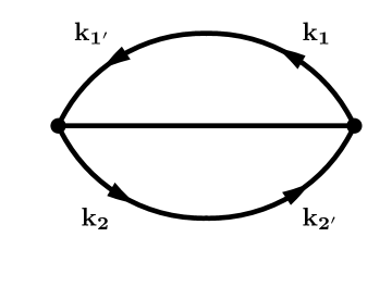
Figure 1: All two body cluster diagrams

The CBS matrix elements can be represented by diagrams, such as those in Figs. 1, 2 and 3, which have been analyzed in detail in FP . We will adopt their notation and use their results. In all the diagrams we use the following conventions.

• The points in these diagrams denote positions of the particles: ${\bf r}_{i},\leavevmode\nobreak\ {\bf r}_{j},...$.

• The dashed lines connecting points $i$ and $j$ represent correlations, i.e. terms originating from ${\cal F}^{2}_{ij}-1$. When ${\cal F}_{ij}=f(r_{ij})$ this notation is sufficient, however, a more elaborate notation for the correlation lines is needed when ${\cal F}$ is an operator with many terms PWRMP . For brevity we will show diagrams assuming ${\cal F}_{ij}=f(r_{ij})$, commonly called the Jastrow correlation function.

• The solid lines represent $v^{eff}_{ij}$. There can only be one solid line in a diagram representing matrix elements of $H$.

• The lines with one or two arrowheads represent state lines. The arrowheads are labeled with quasi-particle states. A state line with a single arrowhead labeled ${\bf k}_{\ell}$ going from point $i$ to point $j$ indicates that the particle $i$ is in state ${\bf k}_{\ell}$ in the ket $|\Psi_{I})$ and particle $j$ is in ${\bf k}_{\ell}$ in the bra $(\Psi_{J}|$. Diagrams representing diagonal CBS matrix elements can have state lines with only one arrowhead, since the state ${\bf k}_{\ell}$ is occupied (or unoccupied) in both the bra and the ket.

  Diagrams contributing to the nondiagonal CBS matrix elements have state lines with two arrowheads. The number of these lines equals the number of quasi-particle states that are different in $(\Psi_{J}|$ and $|\Psi_{I})$. A state line with arrowheads ${\bf k}_{\ell}$ and ${\bf k}_{\ell^{\prime}}$, going from $i$ to $j$ indicates that $i$ is in state ${\bf k}_{\ell}$ in the ket, while $j$ is in state ${\bf k}_{\ell^{\prime}}$ in the bra, and that ${\bf k}_{\ell}$ and ${\bf k}_{\ell^{\prime}}$ are unoccupied in the bra and the ket respectively.

  Only one state line must emerge from a point and only one must end in a point because each particle occupies only one quasi-particle state in the bra and the ket. This implies that the state lines form continuous loops. In direct diagrams the state lines emerge from and end on the same particle, while in exchange diagrams they connect pairs of particles.

• The contribution of a diagram is given by an integral over all the particle coordinates ${\bf r}_{i}$ in the diagram. The integrand contains factors of $(f^{2}(r_{ij})-1)$ for each correlation line, $v^{eff}_{ij}$ for the interaction line, $e^{i{\bf k}_{\ell}\cdot{\bf r}_{i}}/\sqrt{\Omega}$ for each state line $\ell$ emerging from a point ${\bf r}_{i}$ and $e^{-i{\bf k}_{\ell^{\prime}}\cdot{\bf r}_{j}}/\sqrt{\Omega}$ for each state line $\ell^{\prime}$ ending in ${\bf r}_{j}$.

The two-body ($2b$) direct ($d$) and exchange diagrams ($e$) representing the nondiagonal matrix elements (30) are shown in Fig. 1. The contributions of the $2b.v^{eff}$ diagrams are given by

$$2b.v^{eff}.d=\frac{1}{\Omega}\int d^{3}r_{ij}\exp(-i\frac{1}{2}({\bf k}_{1^{\prime}}-{\bf k}_{2^{\prime}})\cdot{\bf r}_{ij})v^{eff}(r)\exp(i\frac{1}{2}({\bf k}_{1}-{\bf k}_{2})\cdot{\bf r}_{ij})\leavevmode\nobreak\ ,$$ (33)

$$2b.v^{eff}.e=-\frac{1}{\Omega}\int d^{3}r_{ij}\exp(-i\frac{1}{2}({\bf k}_{2^{\prime}}-{\bf k}_{1^{\prime}})\cdot{\bf r}_{ij})v^{eff}(r)\exp(i\frac{1}{2}({\bf k}_{1}-{\bf k}_{2})\cdot{\bf r}_{ij})\leavevmode\nobreak\ ,$$ (34)

for spin independent $v$ (and $f$) . The contributions of $2b.{\cal F}^{2}$ diagrams are obtained by replacing $v^{eff}$ by ${\cal F}^{2}-1$. All $2b$ diagrams have a contribution of order $1/\Omega$.

The change in energy, $\delta E_{I}$, [Eq. (26)] contains products of the $2b.v^{eff}$ and $2b.{\cal F}^{2}$ diagrams. These products are of order $1/\Omega^{2}$. The total contribution of the leading $2b$ cluster terms to $\delta E_{I}$ is obtained by summing over the states $\mathbf{k_{1},k_{2},k_{1^{\prime}},k_{2^{\prime}}}$. Each allowed combination of these states corresponds to a many-body state in the set ${\cal M}_{0}$. The quasi-particle states $\mathbf{k_{1}}$ and $\mathbf{k_{2}}$ can be any two of those occupied in $I$. Thus the sum over these gives a factor of order $N^{2}$. Next we sum over $\mathbf{k_{1^{\prime}}}$ and $\mathbf{k_{2^{\prime}}}$. The total momentum ${\bf k}_{1^{\prime}}+{\bf k}_{2^{\prime}}$ is determined from Eq. (29). The magnitude of the relative momentum,

$${\bf k}_{1^{\prime}2^{\prime}}=\frac{1}{2}({\bf k}_{1}^{\prime}-{\bf k}_{2}^{\prime})\leavevmode\nobreak\ ,$$ (35)

is constrained by energy conservation,

$$\epsilon_{V}({\bf k}_{1})+\epsilon_{V}({\bf k}_{2})=\epsilon_{V}({\bf k}_{1^{\prime}})+\epsilon_{V}({\bf k}_{2^{\prime}})\leavevmode\nobreak\ .$$ (36)

required for $J$ to be in the set ${\cal M}_{0}$. Thus the sum over states allowed for $\mathbf{k_{1^{\prime}}}$ and $\mathbf{k_{2^{\prime}}}$ corresponds to an integration over the direction of ${\bf k}_{1^{\prime}2^{\prime}}$. It gives a factor of order $\Omega^{1/3}$. Hence

$$\delta e_{I}.2b = \frac{1}{N}\delta E_{I}.2b$$ (37)

$$\sim \frac{1}{N}\frac{1}{\Omega^{2}}N^{2}\Omega^{1/3}$$ (38)

$$\sim \rho\Omega^{-2/3}$$ (39)

i.e. $\delta e_{I}.2b\rightarrow 0$ as $N\rightarrow\infty$. Note that with the constraint of momentum conservation alone we can integrate over the magnitude of ${\bf k}_{1^{\prime}2^{\prime}}$. This integration gives a factor of order $\Omega$ and makes $\delta e_{I}.2b$ of order $1$. The equal energy constraint in the ECMC ${\cal M}_{0}$ ( Eq. (24)) makes $\delta e_{I}.2b$ vanish in the thermodynamic limit.

The above analysis can be carried out for contribution of clusters with three or more particles to $\delta E_{I}$. Consider, for example, states $J$ which differ from $I$ in occupation numbers of three quasi particles. These states can be reached by scattering three quasi-particles in $I$ in states ${\bf k}_{1},{\bf k}_{2},{\bf k}_{3}$ to states ${\bf k}_{1^{\prime}},{\bf k}_{2^{\prime}},{\bf k}_{3^{\prime}}$ occupied in $J$. The relevant, direct $3b$ diagrams are shown in Fig. 2. Each diagram is of order $1/\Omega^{2}$. The contribution of three body cluster terms to $\delta E_{I}$ are products of $v^{eff}$ and ${\cal F}^{2}-1$ diagrams. Each of these products is of order $1/\Omega^{4}$. We get a factor of order $N^{3}$ by summing over states ${\bf k}_{1},{\bf k}_{2}$ and ${\bf k}_{3}$, and a factor $\Omega^{4/3}$ by summing over $\mathbf{k_{1^{\prime}},k_{2^{\prime}},k_{3^{\prime}}}$ with constraints of momentum and energy conservation. Thus their total contribution to $\delta e_{I}$ is of order $N^{-1}(\Omega^{-4}N^{3}\Omega^{4/3})\sim\rho^{2}\Omega^{-2/3}$ which vanishes in the thermodynamic limit just like the contribution from the leading two body cluster terms. Similarly the contribution from all connected terms can be shown to give vanishing contribution to $\delta e_{I}$ in the thermodynamic limit.

The terms of Eq. (26) will also contain disconnected diagrams like those shown in Fig. 3. These diagrams by themselves will give rise to unphysical divergent (non extensive) contributions to the energy. To extract any physically meaningful result from the theory, these diagrams must cancel identically.

Disconnected diagrams in the expansion for the shift in energy ($\delta E_{I}$) can be classified into two types.

• Diagrams in which each connected cluster conserves energy.

• Diagrams in which only the whole diagram conserves energy, i.e. each connected cluster does not conserve energy.

Let us, consider the first case.

Consider the simplest possible divergent diagrams, i.e. Fig. 3.

Let us denote the CBS $|\Psi_{J})$, $|\Psi_{K})$ and $|\Psi_{L})$ by

$$|\Psi_{J}) = |\mathbf{k_{1^{\prime}},k_{2^{\prime}},k_{3^{\prime}},k_{4^{\prime}}}:I-\mathbf{k_{1},k_{2},k_{3},k_{4}})$$

$$|\Psi_{K}) = |\mathbf{k_{1^{\prime}},k_{2^{\prime}}}:I-\mathbf{k_{1},k_{2}})$$

$$|\Psi_{L}) = |\mathbf{k_{3^{\prime}},k_{4^{\prime}}}:I-\mathbf{k_{3},k_{4}})$$ (40)

Let $\mathbf{k_{1},k_{2}}$ and $\mathbf{k_{1^{\prime}},k_{2^{\prime}}}$ conserve momentum and energy amongst themselves and similarly for $\mathbf{k_{3},k_{4}}$ and $\mathbf{k_{3^{\prime}},k_{4^{\prime}}}$.

$${\bf k}_{1}+{\bf k}_{2}={\bf k}_{1^{\prime}}+{\bf k}_{2^{\prime}}\leavevmode\nobreak\ ,$$ (41)

$${\bf k}_{3}+{\bf k}_{4}={\bf k}_{3^{\prime}}+{\bf k}_{4^{\prime}}\leavevmode\nobreak\ ,$$ (42)

and

$$\epsilon_{V}({\bf k}_{1})+\epsilon_{V}({\bf k}_{2})=\epsilon_{V}({\bf k}_{1^{\prime}})+\epsilon_{V}({\bf k}_{2^{\prime}})\leavevmode\nobreak\ ,$$ (43)

$$\epsilon_{V}({\bf k}_{3})+\epsilon_{V}({\bf k}_{4})=\epsilon_{V}({\bf k}_{3^{\prime}})+\epsilon_{V}({\bf k}_{4^{\prime}})\leavevmode\nobreak\ .$$ (44)

An inspection of the series on the right hand side of Eq. (26) will show that thirteen (13) terms in total will give rise to an integral which will be represented by products of diagrams shown in Fig. 3. In Table 1 we list the terms and also their corresponding prefactor in the series. As one can see, the sum of the prefactors is identically zero. Thus products of diagrams of the type shown in Fig. 3 has no contribution to the change in energy per particle ($\delta e_{I}$). The cancellation of corresponding exchange diagrams and all other divergent diagrams of this order with three or more body connected pieces can also be shown to cancel with analogous book keeping. The divergent diagrams of the next highest order can also be shown to cancel identically.

Now consider the case when the individual clusters do not conserve energy, i.e. Eqs. (41, 42) are still true but Eqs. (43, 44) are not true. Instead,

$$\epsilon_{V}({\bf k}_{1})+\epsilon_{V}({\bf k}_{2})+\epsilon_{V}({\bf k}_{3})+\epsilon_{V}({\bf k}_{4})=\epsilon_{V}({\bf k}_{1^{\prime}})+\epsilon_{V}({\bf k}_{2^{\prime}})+\epsilon_{V}({\bf k}_{3^{\prime}})+\epsilon_{V}({\bf k}_{4^{\prime}})\leavevmode\nobreak\ .$$ (45)

In this case the states $K$ and $L$ no longer belong to the same ECMC as $I$ and $J$. Thus, none of the terms in Table 1, except for the first, will be included in the sum, i.e. the divergent terms, $\left(\Psi_{I}\right|v^{eff}\left|\Psi_{J}\right)\left(\Psi_{J}\right.\left|\Psi_{I}\right)$ and its complex conjugate will not get cancelled. The total contribution of terms like these to $\delta E_{I}$ is of order $\rho^{4}\Omega^{4/3}$, i.e. the shift in the energy per particle, $\delta e_{I}\sim\rho^{3}\Omega^{1/3}$, diverges in the thermodynamic limit.

The survival of divergent terms is rather artificial and arises from the sharp energy conservation constraint that we imposed on the states in ${\cal M}_{0}$. This provides the motivation to define a ensemble where this constraint is relaxed slightly. In what follows we will show that this can be done consistently where none of the divergent terms are present while the diagonal matrix elements of the Hamiltonian are preserved.

II.2 The set of Most Probable Distributions (MPD)

Consider an ideal gas of fermions in a box of volume $L^{3}(=\Omega)$ . The single particle energy levels are given by

$$\epsilon_{V}(\mathbf{n}_{i})=\frac{\hbar^{2}}{2m}\frac{{\mathbf{n}}_{i}^{2}}{2\pi L^{2}}$$ (46)

where $m$ is the mass of the fermions and ${\mathbf{n}}_{i}$ is a vector with integer components. In what follows we will use units where $\frac{\hbar^{2}}{4\pi m}=1$. Let the total number of particles in the box be $N$.

The density of states at any single particle energy $\epsilon_{V}$ is given by

$$g(\epsilon_{V})\sim L^{3}\epsilon_{V}^{1/2}$$ (47)

Now consider a cell with an energy width of $\frac{\Delta}{L^{2}}$, around an energy level $\epsilon_{V}$ . Then the number of single particle energy levels in this cell is

$$\omega(\epsilon_{V})\sim g(\epsilon_{V})\frac{\Delta}{L^{2}}\sim L^{3}\epsilon_{V}^{1/2}\frac{\Delta}{L^{2}}\leavevmode\nobreak\ .$$ (48)

The exact value of $\Delta$ is not important, except for the fact that it is dimensionless and of order 1 or less. We can always choose $\Delta$ so that $\omega(\epsilon_{V})$ is large,

$$\omega(\epsilon_{V})\gg 1\leavevmode\nobreak\ .$$ (49)

Let the total number of particles in the energy cell around $\epsilon_{V}$ be $n(\epsilon_{V})$. Let $S({n(\epsilon_{V})})$ be the entropy corresponding to the configuration (distribution) $n(\epsilon_{V})$. It can be easily shown that the entropy, $S_{V}$ corresponding to the most probable distribution of number of particles per energy cell , subject to the constraints

$$\sum n(\epsilon_{V}) = N$$ (50)

$$\textrm{and}\qquad\sum\epsilon_{V}n(\epsilon_{V}) = E_{MC}\leavevmode\nobreak\ ,$$ (51)

is given by Eq. (12), i.e., the distribution $\overline{n}(\epsilon_{V})$ in addition to satisfying Eqs. (50,51) also satisfies the maximization condition,

$$S(\overline{n}(\epsilon_{V}))=\textrm{Maximum}(S(n(\epsilon_{V})))$$ (52)

The temperature and the chemical potential are the Lagrange multipliers of the minimization procedure. Now we will define our microcanonical ensemble as the set ${\cal M}$ of all configurations whose cell distribution is ${\overline{n}(\epsilon_{V})}$. We will call this the set of Most Probable Distributions (MPD). Please note that this is different from defining an ensemble with total energy $E_{\textrm{MC}}$, but is roughly the same as defining an ensemble with an average energy $E_{\textrm{MC}}$ and a small non zero energy width $\delta E_{\textrm{MC}}$.

$${\cal M}\equiv\bigcup(\textrm{ All states with the distribution }{\overline{n}(\epsilon_{V})})$$ (53)

It should be emphasized here that none of the conclusions that follow depend explicitly on the actual single particle spectrum given by Eq. (46). All the conclusions remain unchanged as long as the single particle energy levels produce a continuum in the thermodynamic limit. However we will continue to use Eq. (46) because the calculations are more transparent this way.

The probability of fluctuations about the most probable distribution is given by Einstein’s relation,

$$P(\delta n)\sim e^{-\delta S}\leavevmode\nobreak\ ,$$ (54)

where $P(\delta n)$ is the probability of a fluctuation of size $\delta n$ and $\delta S$ is the corresponding decrease in entropy. Around the most probable distribution,

$$\delta S\sim\delta n^{2}\leavevmode\nobreak\ ,$$ (55)

i.e. the probability of fluctuations vanishes exponentially with the size of the fluctuations.

In addition, the fluctuation (standard deviation) in the value of the total energy, $E^{V}_{I}$, in ${\cal M}$, can be easily shown to be,

$$\delta E<\frac{\Delta}{L^{2}}\sqrt{N}$$ (56)

i.e. $\delta E$ is non macroscopic; the fluctuation in the energy per particle vanishes in the thermodynamic limit. Thus, the ensemble we have defined is a consistent one in the statistical sense.

Now let us discuss the allowed scattering processes within the set ${\cal M}$. For two states to be in ${\cal M}$, they must have the same populations $n(\epsilon_{V})$ in all the energy bins (cells). What this means is that they must be connected to each other through excitations within cells. For example let $I$ and $\mathbf{k_{1^{\prime}},k_{2^{\prime}}}:I-\mathbf{k_{1},k_{2}}$, be elements of ${\cal M}$. Let

$$\epsilon_{V}(\mathbf{k_{1}}) \leq \epsilon_{V}(\mathbf{k_{2}})$$ (57)

$$\textrm{and}\qquad\epsilon_{V}(\mathbf{k_{1^{\prime}}}) \leq \epsilon_{V}(\mathbf{k_{2^{\prime}}})\leavevmode\nobreak\ .$$ (58)

Then, we need to have

$$|\epsilon_{V}(\mathbf{k_{1^{\prime}}})-\epsilon_{V}(\mathbf{k_{1}})| < \frac{\Delta_{1}}{L^{2}}$$ (59)

$$\textrm{and}\qquad|\epsilon_{V}(\mathbf{k_{2^{\prime}}})-\epsilon_{V}(\mathbf{k_{2}})| < \frac{\Delta_{2}}{L^{2}}$$ (60)

where $\frac{\Delta_{1}}{L^{2}}$ and $\frac{\Delta_{2}}{L^{2}}$ are the widths of the cells containing $\mathbf{k_{1}}$ and $\mathbf{k_{2}}$ respectively. Please note that this, in general, means that there is no exact energy conservation, but that there is approximate energy conservation for each individual particle.

Let us discuss the orthogonalization correction in ${\cal M}$. Consider the disconnected diagrams first. Following the discussion before, let us define states $J$, $K$ and $L$ as in Eq. (II.1), with,

$$\epsilon_{V}(\mathbf{k_{1}})\leq\epsilon_{V}(\mathbf{k_{2}})\leq\epsilon_{V}(\mathbf{k_{3}})\leq\epsilon_{V}(\mathbf{k_{4}})\leavevmode\nobreak\ ,$$

$$\epsilon_{V}(\mathbf{k_{1^{\prime}}})\leq\epsilon_{V}(\mathbf{k_{2^{\prime}}})\leq\epsilon_{V}(\mathbf{k_{3^{\prime}}})\leq\epsilon_{V}(\mathbf{k_{4^{\prime}}})\leavevmode\nobreak\ .$$ (61)

Let us assume that they obey Eqs. (41, 42) i.e. they form two disconnected momentum conserving clusters.

Now it is crucial to observe that if $I$ and $J$ belong to ${\cal M}$ then $\mathbf{k_{1}}$ and $\mathbf{k_{1^{\prime}}}$ must belong to the same energy cell; similarly for ${\bf k}_{2}$ and ${\bf k}_{2^{\prime}}$, ${\bf k}_{3}$ and ${\bf k}_{3^{\prime}}$ , and ${\bf k}_{4}$ and ${\bf k}_{4^{\prime}}$. This implies that $K$ and $L$ must also belong to ${\cal M}$. This was not the case when we had merely imposed overall exact energy conservation.

Thus, in this case all the terms in Table 1 will contribute to the sum in Eq. (26). As such the disconnected diagrams will cancel each other and we will be left with a connected, non divergent sum, i.e.

$$\delta E^{\textrm{disconnected}}_{I}=0$$ (62)

identically. The problem with disconnected diagrams that we encounter in ECMC is resolved in MPD.

For the sake of completeness, we show that the connected diagrams also have a vanishing contribution towards the energy in the thermodynamic limit. Consider the two body cluster contributions to $\delta E_{I}$. The $\delta E_{I}$ [Eq. (26)] contains products of the $2b.v^{eff}$ and $2b.{\cal F}^{2}$ diagrams. These products are of order $1/\Omega^{2}$. The total contribution of the leading 2b cluster terms to $\delta E_{I}$ is obtained by summing over the states $\mathbf{k_{1}}$, $\mathbf{k_{2}}$, $\mathbf{k_{1^{\prime}}}$ and $\mathbf{k_{2^{\prime}}}$. Each allowed combination of these states corresponds to a many-body state in the set ${\cal M}$. The quasi-particle states $\mathbf{k_{1}}$ and $\mathbf{k_{2}}$ can be any two of those occupied in $I$. Thus, the sum over $\mathbf{k_{1}}$ and $\mathbf{k_{2}}$ gives a factor of order $N^{2}$. Next we sum over $\mathbf{k_{1^{\prime}}}$ and $\mathbf{k_{2^{\prime}}}$. The total momentum ${\bf k}_{1^{\prime}}+{\bf k}_{2^{\prime}}$ is determined from Eq. (29). The magnitude of the relative momentum:

$${\bf k}_{1^{\prime}2^{\prime}}=\frac{1}{2}({\bf k}_{1}^{\prime}-{\bf k}_{2}^{\prime})\leavevmode\nobreak\ ,$$ (63)

is constrained by Eqs. (59, 60).

The sum over states allowed for $\mathbf{k_{1^{\prime}}}$ and $\mathbf{k_{2^{\prime}}}$ corresponds to an integration over ${\bf k}_{1^{\prime}2^{\prime}}$. But ${\bf k}_{1^{\prime}2^{\prime}}$ is constrained to lie in a shell of width $\Delta$ where, $\Delta\sim\min(\Delta_{1},\Delta_{2})$. Thus, the sum over ${\bf k}_{1^{\prime}}$ and ${\bf k}_{2^{\prime}}$ gives a contribution $\sim\Omega\frac{\Delta}{L^{2}}$ up to a factor of order 1 (the factor of $\Omega$ comes from the density of states). Therefore the total contribution of the 2b diagrams after summing over $\mathbf{k_{1},k_{2},k_{1^{\prime}},k_{2^{\prime}}}$ is,

$$\delta E_{I}.2b\sim\Omega\rho^{2}\frac{\Delta}{L^{2}}\leavevmode\nobreak\ .$$ (64)

Thus the shift in the energy per particle is,

$$\delta e_{I}.2b\sim\rho\frac{\Delta}{L^{2}}\leavevmode\nobreak\ ,$$ (65)

which vanishes in the thermodynamic limit.

The above analysis can be easily carried out for contribution of connected clusters with three or more particles to the $\delta E_{I}$. Consider for example states $J$ which differ from $I$ in occupation numbers of three quasi particles. These states can be reached by scattering three quasi-particles in $I$ in states $\mathbf{k_{1},k_{2},k_{3}}$ to states $\mathbf{k_{1^{\prime}},k_{2^{\prime}},k_{3^{\prime}}}$ occupied in $J$. For example consider the direct 3b term shown in Fig. 2 . Each is of order $1/\Omega^{2}$, thus their contribution to $\delta E_{I}$ is of order $1/\Omega^{4}$. We get a factor of order $N^{3}$ by summing over $\mathbf{k_{1},k_{2},k_{3}}$, and a factor $\Omega^{2}\left(\frac{\Delta}{L^{2}}\right)^{2}$ by summing over $\mathbf{k_{1^{\prime}},k_{2^{\prime}},k_{3^{\prime}}}$ with constraints of momentum and (approximate) energy conservation. Thus their total is of order $\Omega\rho^{3}\left(\frac{\Delta}{L^{2}}\right)^{2}$. The contribution to the shift in energy per particle is $\delta e_{I}\sim\rho^{2}\left(\frac{\Delta}{L^{2}}\right)^{2}$ which vanishes in the thermodynamic limit: similarly for higher order clusters. Therefore, for connected clusters we see that

$$\delta e_{I}^{\textrm{connected}}\rightarrow 0\leavevmode\nobreak\ ,$$ (66)

in the thermodynamic limit.

Thus, as claimed earlier in the section we have shown that it is possible to define a statistically consistent microcanonical ensemble such that Eq. (19) is true for the elements in the microcanonical ensemble ${\cal M}$.

II.3 Discussion

The simplest choice for a microcanonical ensemble is the ECMC. The ECMC has the following properties:

• The states in ECMC have exact energy conservation; this imposes a sharp energy cutoff.

• Arbitrarily high single particle energy transfers are allowed while still remaining in the same ECMC

It is due to the second property that clusters in disconnected diagrams can have arbitrary energy transfers and hence divergent contributions. These contributions are normally (in a canonical ensemble, when all states are included) canceled by contributions from higher order terms. But by imposing exact energy conservation we exclude the states which lead to these higher order terms which cancel the divergent part. Thus, we are left with a divergent series.

In MPD on the one hand we relax the energy conservation slightly, and on the other hand we limit single particle energy transfers to the width of the energy cells. We showed that this leads to a convergent series. Also, we showed that the total energy is well defined in a MPD and that states with large deviations from the MPD (i.e. states with large single particle energy transfers) are exponentially improbable.

The main difference between ECMC and MPD is that one follows from a conservation law and the other from a distribution. There can be states in the ECMC whose population distribution in the energy cells is very different from the MPD $\overline{n}(\epsilon_{V})$, but as long as the total energy of the state, $E_{V}=E_{MC}$, this state is a valid member of the ECMC. However, the number of these states is negligible as compared to the total number of states which have the MPD, and hence they can be safely neglected in the thermodynamic limit. On the other hand, those states whose total energy $E_{V}$ differ from $E_{MC}$ by a non macroscopic amount and have the same population distribution as the MPD should be included in the microcanonical ensemble. We have shown that, for our purposes, a typical state in a microcanonical ensemble is given by the (most probable) distribution and not by an exact conservation law.

Thus, we have shown that a consistent choice for ${\cal M}$ does exist. We have also shown that the most obvious choice, namely, the ECMC leads to divergences in the theory. We traced these divergences to the existence of the sharp cutoff due to the exact energy conservation imposed on the states. Then we showed that these unphysical divergences can be removed by relaxing the energy conservation slightly, with the set of MPDs. We showed that MPDs can be consistently treated as microcanonical ensembles and that the diagonal matrix elements of the Hamiltonian remain unchanged upon orthogonalization in this ensemble.

In practical calculations, a microcanonical sample, ${\cal M}$ of CBS is given by

$$|\Psi_{MC}) = |\Psi\{n_{MC}({\bf k},\sigma_{z})\})\leavevmode\nobreak\ ,$$ (67)

$$n_{MC}({\bf k},\sigma_{z}) = 1\leavevmode\nobreak\ \textrm{with probability}\leavevmode\nobreak\ \overline{n}({\bf k},\sigma_{z});\leavevmode\nobreak\ \textrm{else zero}\leavevmode\nobreak\ .$$ (68)

The state $|\Psi_{MC})$ (Eq. 67) belongs to the MC ensemble with energy

$$E_{V,MC}=\sum_{\sigma_{z}}\int\frac{d^{3}k}{(2\pi)^{3}}n_{MC}({\bf k},\sigma_{z})\epsilon_{V}({\bf k},\sigma_{z})\leavevmode\nobreak\ .$$ (69)

Since the Hamiltonian $H_{V}$ can be easily solved, we can find the temperature corresponding to this energy. In the $N\rightarrow\infty$ limit it is just that used to find the $\overline{n}({{\bf k},\sigma_{z}})$ [Eq. (10)]. All the MC states belonging to this set can be found by allowing particles in $|\Psi_{MC})$ to scatter into allowed final states. Each scattering produces a new CBS belonging to the same MC set. We denote this set by ${\cal M}$. If the quantum liquid is contained in a thin container with negligible specific heat, then it passes through the states in ${\cal M}$ when in equilibrium at temperature $T$ and density $\rho$.

Eqs. (67, 68) have been recently used to calculate the rates of weak interactions in hot nuclear matter  CP05 . Note that $|\Psi_{MC})$ is a CBS since $n_{MC}({\bf k},\sigma_{z})$ are either 1 or 0. When the number of particles in $|\Psi_{MC})$ is large the fluctuations due to sampling the probability distribution $\overline{n}({\bf k},\sigma_{z})$ are negligible, and this state has the desired densities $\rho_{\pm}$ and energy per particle appropriate for the desired temperature $T$ and Hamiltonian $H_{V}$ used to calculate the $\overline{n}$. Neglecting these fluctuations in the limit $N\rightarrow\infty$ we obtain the variational estimate for the free energy,

$$F_{V}(\rho,T)=\textrm{minimum of}\leavevmode\nobreak\ \big{[}(\Psi_{MC}|H|\Psi_{MC})-TS_{V}(\rho,T)\big{]}\leavevmode\nobreak\ ,$$ (70)

where the minimum value is obtained by varying the ${\cal G}$ and $\epsilon_{V}({\bf k},\sigma_{z})$. The $(\Psi_{MC}|H|\Psi_{MC})$ can be calculated with standard cluster expansion and chain summation methods used in variational theories of cold quantum liquids PWRMP ; mpr . At low temperatures ($\ll T_{F}$) this method is particularly simple because the zero temperature ${\cal G}$ and $\epsilon({\bf k},\sigma_{z})$ provide very good approximations to the optimum. The main concerns raised in past applications FPS ; FP81 of the SP scheme is that it neglects the nonorthogonality of the CBS, and provides only upperbounds for the free energy. Here we address only the first. At zero temperature the difference between the variational and the exact ground state energy has been estimated with correlated basis perturbation theory FFP . It may be possible to extend these methods to finite temperatures.

III Orthonormalization of the quasiparticle-quasihole excitations

In the calculation of nuclear response functions one needs to use the diagonal matrix elements of the Hamiltonian in the quasiparticle-quasihole states FPRF . At least at zero temperature the leading contribution to the dynamic structure function comes the 1p-1h states. Here we will limit our discussion to the diagonal matrix elements of the Hamiltonian in the 1p-1h excitations from the states in ${\cal M}$.

Consider a OCBS $|\Psi_{I}\rangle$, $I\in{\cal M}$, where the single quasiparticle state with momentum $\mathbf{h}$ is occupied but the single quasiparticle state with momentum $\mathbf{h+k}$ is not. We will denote the quasiparticle-quasihole OCBS where the quasiparticle state with momentum $\mathbf{h}$ is replaced by one with momentum $\mathbf{h+k}$ by $|\mathbf{h+k}:I-\mathbf{h}\rangle$, and the corrresponding CBS by $|\mathbf{h+k}:I-\mathbf{h})$. The CBS $|\mathbf{h+k}:I-\mathbf{h})$ is orthogonal to all the states in ${\cal M}$, because they have different total momenta. Thus it only needs to be orthonormalized with all the other quasiparticle-quasihole excitations with the same momentum, via the Löwdin method. The excitations with two or more quasiparticles and quasiholes should be orthonormalized with the quasiparticle-quasihole states using a sequential method. But this does not have any effect on the quasiparticle-quasihole states, so we do not discuss them any further.

The quasiparticle-quasihole OCBS is given by

$$|\mathbf{h+k}:I-\mathbf{h}\rangle=|\mathbf{h+k}:I-\mathbf{h})-\frac{1}{2}\sum_{I^{\prime}\in{\cal M}}|\mathbf{h^{\prime}+k}:I^{\prime}-\mathbf{h^{\prime}})\left(\mathbf{h^{\prime}+k}:I^{\prime}-\mathbf{h^{\prime}}|\mathbf{h+k}:I-\mathbf{h}\right)+\cdots\leavevmode\nobreak\ ,$$ (71)

where $h^{\prime}\in I^{\prime}$. The diagonal matrix elements of $H$ are given by

$$\langle\mathbf{h+k}:I-\mathbf{h}|H|\mathbf{h+k}:I-\mathbf{h}\rangle = \left(\mathbf{h+k}:I-\mathbf{h}|H|\mathbf{h+k}:I-\mathbf{h}\right)$$ (72)

$$- \frac{1}{2}\sum_{I^{\prime}\in{\cal M}}\left[\left(\mathbf{h+k}:I-\mathbf{h}|H|\mathbf{h^{\prime}+k}:I^{\prime}-\mathbf{h^{\prime}}\right)\right.$$

$$\times \left.\left(\mathbf{h^{\prime}+k}:I^{\prime}-\mathbf{h^{\prime}}|\mathbf{h+k}:I-\mathbf{h}\right)+c.c.\right]+\cdots$$

In actual calculation of response functions one needs the difference between $\langle\mathbf{h+k}:I-\mathbf{h}|H|\mathbf{h+k}:I-\mathbf{h}\rangle$ and $\langle\Psi_{I}|H|\Psi_{I}\rangle$. Let us define

$$E_{ph}=\left[\langle\mathbf{h+k}:I-\mathbf{h}|H|\mathbf{h+k}:I-\mathbf{h}\rangle-\langle\Psi_{I}|H|\Psi_{I}\rangle\right]\leavevmode\nobreak\ .$$ (73)

At zero temperature, in accordance with Landau’s theory, one can define single particle energies for quasiparticle and quasiholes as done in Eq. 3. The quantity $E_{ph}$ is analogous to (i.e. is a finite temperature generalization of) the difference between the quasiparticle energy, $\epsilon_{0}(\mathbf{h+k})$, and the quasihole energy, $\epsilon_{0}(\mathbf{h})$. We will show that $E_{ph}$ has no orthogonality corrections.

The orthogonality correction to $E_{ph}$ is given by

$$\delta E_{ph} = \left[\langle\mathbf{h+k}:I-\mathbf{h}|H|\mathbf{h+k}:I-\mathbf{h}\rangle-\langle\Psi_{I}|H|\Psi_{I}\rangle\right]$$

$$- \left[\left(\mathbf{h+k}:I-\mathbf{h}|H|\mathbf{h+k}:I-\mathbf{h}\right)-\left(\Psi_{I}|H|\Psi_{I}\right)\right]$$

$$= \left[\frac{1}{2}\sum_{I^{\prime}\in{\cal M}}\left[\left(\mathbf{h+k}:I-\mathbf{h}|v^{eff}|\mathbf{h^{\prime}+k}:I^{\prime}-\mathbf{h^{\prime}}\right)\left(\mathbf{h^{\prime}+k}:I^{\prime}-\mathbf{h^{\prime}}|\mathbf{h+k}:I-\mathbf{h}\right)\right.\right.$$

$$+ \left.\left.\textrm{c.c.}\right]+\cdots\right]$$

$$- \left[\frac{1}{2}\sum_{I^{\prime}\in{\cal M}}\left[\left(\mathbf{h}:I-\mathbf{h}|v^{eff}|\mathbf{h^{\prime}}:I^{\prime}-\mathbf{h^{\prime}}\right)\left(\mathbf{h^{\prime}}:I^{\prime}-\mathbf{h^{\prime}}|\mathbf{h}:I-\mathbf{h}\right)\right.\right.$$

$$+ \left.\left.\textrm{c.c.}\right]+\cdots\right]$$ (75)

The non diagonal matrix elements of the Hamiltonian ($v^{eff}$) and unity in the second equation are of order $1/\Omega$ or less.

The shift $\delta E_{ph}$ will contain both connected and disconnected terms. The disconnected terms can be shown to cancel exactly using arguments similar to the ones used in the last section. We will consider the connected terms only.

The state $|\mathbf{h^{\prime}+k}:I^{\prime}-\mathbf{h^{\prime}})$ can be of the following types:

• Type 1 : $\mathbf{h^{\prime}}=\mathbf{h}$ , $I^{\prime}\neq I$

• Type 2 : $\mathbf{h^{\prime}}\neq\mathbf{h}$.

For Type 1 terms, the terms of the matrix elements $\left(\mathbf{h+k}:I-\mathbf{h}|v^{eff}|\mathbf{h+k}:I^{\prime}-\mathbf{h^{\prime}}\right)$ and $\left(\mathbf{h+k}:I^{\prime}-\mathbf{h}|\mathbf{h+k}:I-\mathbf{h}\right)$ do not depend on $\mathbf{k}$. (The contribution of the terms which contain the exchange line $\mathbf{h+k}$ vanish in the thermodynamic limit as compared to the leading order terms. This can be easily seen by explicitly writing down the cluster expansion for the matrix elements.) Thus the contribution of these matrix elements is canceled by the corresponding terms $\left(\mathbf{h}:I-\mathbf{h}|v^{eff}|\mathbf{h}:I^{\prime}-\mathbf{h}\right)$ and $\left(\mathbf{h}:I^{\prime}-\mathbf{h}|\mathbf{h}:I-\mathbf{h}\right)$.

Consider the Type 2 CBS. Let $\mathbf{h_{1}}$ be the single quasiparticle state in $I^{\prime}$ which is in the same energy cell (as defined in the last section) as $\mathbf{h}$, and let $\mathbf{h^{\prime}_{1}}$ be the single quasiparticle state in $I$ which is in the same energy cell as $\mathbf{h^{\prime}}$. Since both $I$ and $I^{\prime}$ belong to ${\cal M}$, there will be at least one choice for $\mathbf{h_{1}}$ and $\mathbf{h^{\prime}_{1}}$, although in general their choice is not unique.

$$|\mathbf{h^{\prime}+k}:I^{\prime}-\mathbf{h^{\prime}})\equiv|\mathbf{h^{\prime}+k,h_{1}}:I^{\prime}-\mathbf{h^{\prime},h_{1}})\leavevmode\nobreak\ .$$ (76)

Similarly $|\mathbf{h+k}:I-\mathbf{h})$ can be written as $|\mathbf{h+k,h^{\prime}_{1}}:I-\mathbf{h,h^{\prime}_{1}})$. For Type 2 CBS the leading contribution to Eq. (III) comes from states where $I^{\prime}-\mathbf{h^{\prime},h_{1}}\equiv I-\mathbf{h,h^{\prime}_{1}}$. In this case each of the matrix elements $\left(\mathbf{h+k,h^{\prime}_{1}}:I-\mathbf{h,h^{\prime}_{1}}|v^{eff}|\mathbf{h^{\prime}+k,h_{1}}:I^{\prime}-\mathbf{h^{\prime},h_{1}}\right)$ and $\left(\mathbf{h^{\prime}+k,h_{1}}:I^{\prime}-\mathbf{h^{\prime},h_{1}}|\mathbf{h+k,h^{\prime}_{1}}:I-\mathbf{h,h^{\prime}_{1}}\right)$ are $1/\Omega$. Also, $\mathbf{h^{\prime}_{1}}$ can be any of the occupied quasiparticle states in $I$. Hence summing over $\mathbf{h^{\prime}_{1}}$ gives a factor of $N$. The sum over $\mathbf{h^{\prime}}$ and $\mathbf{h_{1}}$ along with momentum conservation and approximate energy conservation gives a term of order $\Omega\frac{\Delta}{L^{2}}$. Note that there is no summation over $\mathbf{h}$. Thus the total leading order contribution from the Type 2 states is of order $\rho\frac{\Delta}{L^{2}}$, which vanishes in the thermodynamic limit.

Thus,

$$\delta E_{ph}\rightarrow 0\leavevmode\nobreak\ .$$ (77)

There is no orthogonality correction to the energy differences which enter the calculations of response functions.

IV Conclusion

We have developed a variational theory for hot quantum liquids. We have shown that the correlated basis states which provide a reasonable description of the ground state of quantum liquids can be used to describe quantum liquids at finite temperature. Although the correlated basis states are not orthogonal to each other by construction, the free energy calculated in a suitably defined microcanonical ensemble of the correlated basis does not have any corrections due to nonorthogonality. As such the powerful cluster expansion and chain summation methods developed for zero temperature quantum liquids can be used at finite temperature without any reformulation. We have also shown that the energy differences which are needed for calculating response functions do not need any orthogonality corrections either.

We wish to emphasize that the arguments used in this work do not depend on the detailed form of the correlation functions or the choice of the trial single quasiparticle spectrum. The correlated functions are merely required to be sufficiently well behaved so that all the integrals used in the Sections II and III are finite. Any reasonable form for the correlation functions can be expected to satisfy this requirement. Although we have used only two body correlation functions without any state dependence or backflow terms to illustrate our results, the arguments can be easily extended to include both of the above and also three body correlations. Similarly, the arguments can also be extended for any trial single particle spectrum which has a vanishing energy level spacing in the thermodynamic limit.

We have not addressed the problem of non diagonal matrix elements, which are required for certain applications. One such case is presented in the calculation of weak interaction rates, where the relevant matrix elements are the non diagonal matrix elements of one body operators. Work is in progress to calculate the non diagonal matrix elements of these one body weak interaction operators including the orthogonality corrections.

We have also not discussed the actual forms for the correlation functions or the trial single quasiparticle spectrum which may be useful for calculating the free energy at finite temperature. At low enough temperatures the zero temperature forms may provide good approximations, but at higher temperature this is probably not true. Methods to optimize free energy computations at finite temperature are being developed.

Term	Prefactor
$\left(\Psi_{I}\right|v^{eff}\left|\Psi_{J}\right)(\Psi_{J}|\Psi_{I})$	$-\frac{1}{2}$
$(\Psi_{I}|v^{eff}|\Psi_{J})(\Psi_{J}|\Psi_{L})(\Psi_{L}|\Psi_{I})$	$\frac{3}{8}$
$(\Psi_{I}|v^{eff}|\Psi_{K})(\Psi_{K}|\Psi_{L})(\Psi_{L}|\Psi_{I})$	$\frac{3}{8}$
$(\Psi_{I}|v^{eff}|\Psi_{J})(\Psi_{J}|\Psi_{K})(\Psi_{K}|\Psi_{I})$	$\frac{3}{8}$
$(\Psi_{I}|v^{eff}|\Psi_{K})(\Psi_{K}|\Psi_{J})(\Psi_{J}|\Psi_{I})$	$\frac{3}{8}$
$(\Psi_{I}|v^{eff}|\Psi_{K})(\Psi_{K}|\Psi_{J})(\Psi_{J}|\Psi_{K})(\Psi_{K}|\Psi_{I})$	$-\frac{5}{16}$
$(\Psi_{I}|v^{eff}|\Psi_{K})(\Psi_{K}|\Psi_{J})(\Psi_{J}|\Psi_{L})(\Psi_{L}|\Psi_{I})$	$-\frac{5}{16}$
$(\Psi_{I}|v^{eff}|\Psi_{K})(\Psi_{K}|\Psi_{I})(\Psi_{I}|\Psi_{L})(\Psi_{L}|\Psi_{I})$	$-\frac{5}{16}$
$(\Psi_{I}|\Psi_{L})(\Psi_{L}|v^{eff}|\Psi_{J})(\Psi_{J}|\Psi_{I})$	$\frac{1}{4}$
$(\Psi_{I}|\Psi_{L})(\Psi_{L}|v^{eff}|\Psi_{K})(\Psi_{K}|\Psi_{I})$	$\frac{1}{4}$
$(\Psi_{I}|\Psi_{L})(\Psi_{L}|v^{eff}|\Psi_{J})(\Psi_{J}|\Psi_{L})(\Psi_{L}|\Psi_{I})$	$-\frac{3}{16}$
$(\Psi_{I}|\Psi_{L})(\Psi_{L}|v^{eff}|\Psi_{J})(\Psi_{J}|\Psi_{K})(\Psi_{K}|\Psi_{I})$	$-\frac{3}{16}$
$(\Psi_{I}|\Psi_{L})(\Psi_{L}|\Psi_{I})(\Psi_{I}|v^{eff}|\Psi_{K})(\Psi_{K}|\Psi_{I})$	$-\frac{3}{16}$
Total	$0$

Table 1: The contribution of all the terms which give rise to a term like Fig. 3

Figure 2: Examples of three body connected diagrams

Figure 3: Examples of disconnected diagrams