Thermodynamic properties of nuclear matter
at finite temperature

Abstract

Thermodynamic quantities in symmetric nuclear matter are calculated in a self-consistent $T-$matrix approximation at zero and finite temperatures. The internal energy is calculated from the Galitskii-Koltun’s sum rule and from the summation of the diagrams for the interaction energy. The pressure and the entropy at finite temperature are obtained from the generating functional form of the thermodynamic potential.

21.30.Fe, 21.65.+f, 24.10.Cn

1 Introduction

Nuclear matter is studied as a many-body system of interacting fermions. Its equation of state is of particular interest because of its applications to heavy-ion collisions, supernovae collapses and neutron stars structure. The thermodynamic properties of such systems can be investigated starting from the nucleon-nucleon potential; strong interactions between nucleons induce short range correlations in the dense nuclear matter.

Our approach is based on finite-temperature Green’s functions. We adopt the $T-$matrix approximation [1], which consists in expressing the self-energy as a sum of ladder diagrams. Such a self-consistent scheme belongs to a class of approximations derivable from a suitably chosen generating functional [1, 2], which automatically fulfill thermodynamic relations, including the Hugenholz-Van Hove and Luttinger identities [3, 4].

For what concerns the binding energy at zero temperature the thermodynamically consistent $T-$matrix approximation [5, 6] yields results similar to other approaches, such as extensive variational and Brueckner-Hartree-Fock calculations [7, 8]. It is hazardous to compute the pressure and the entropy simply by integrating thermodynamic relations because of uncontrollable numerical errors that propagate at small temperatures. We present instead a method which allows to reliably calculate the pressure (and consequently the entropy) at sufficiently high temperatures from the diagrammatic expansion of the thermodynamic potential [9].

The starting point of these studies is a free N-N potential, a parameterization of the interaction derived from nucleon-nucleon scattering experiments. In the present paper we restrict ourselves to the two-body CD-Bonn potential and will consider three-body interactions in a future work.

2 $T-$matrix approximation

In the in-medium $T-$matrix approach the two-particle propagator takes the following form (for simplicity we skip spin and isospin indices, as well as energy and momentum dependence)

$$\mathcal{G}_{2}=G_{2}^{nc}+G_{2}^{nc}\>T\>G_{2}^{nc}+\>exchange\>terms\>\>.$$ (1)

$G_{2}^{nc}$ is the non correlated two-particle Green’s function, just constructed as a product of two dressed single-particle propagators. We remark that the use of the dressed propagator implies the presence of a nontrivial dispersive self-energy which leads to a broad spectral function [10]. The in-medium two-particle scattering matrix $T$, which appears in the above expression, is defined as

$$T=V+V\>G_{2}^{nc}\>T$$ (2)

where $V$ is the interaction potential. All the ingredients are then calculated iteratively: the scattering matrix, the single-particle self-energy, which is expressed in terms of the scattering matrix, and the single-particle propagator, by means of the Dyson equation.

The $T-$matrix approximation scheme can be as well derived from a generating functional $\Phi[G,V]$ which is a set of two-particle irreducible diagrams [2] obtained by closing two-particle ladder diagrams with a combinatorial factor $1/2n$, where $n$ is the number of interaction lines in the diagram.

Figure 1: Two-particle irreducible functional for the $T-$matrix approximation. The sum runs over the number of interaction lines $n$ in the two-particle ladders.

The functional $\Phi$ depends on the dressed propagators (lines in Fig. 1) and on the two-particle potential (wavy lines in Fig. 1). The self-energy is then expressed as a functional derivative $\displaystyle\Sigma=\frac{\delta\Phi}{\delta G}$.

3 Properties of the correlated system

3.1 Internal energy

The (total) internal energy per particle can be calculated as the expectation value of the Hamiltonian of the system $H=H_{kin}+H_{pot}$

$$\frac{E}{N}=\frac{1}{\rho}\left[\frac{\langle H_{kin}\rangle}{\mathcal{V}}+\frac{\langle H_{pot}\rangle}{\mathcal{V}}\right]\>.$$ (3)

Here $\rho$ is the density and $\mathcal{V}$ the volume of the system. When we evaluate the right hand side of (3) in momentum space we see that the kinetic part is

$$\langle H_{kin}\rangle=\mathcal{V}\int\frac{d^{3}{p}}{(2\pi)^{3}}\frac{d\omega}{2\pi}\frac{\mathbf{p}^{2}}{2m}A(\mathbf{p},\omega)f(\omega)\>,$$ (4)

where $A(\mathbf{p},\omega)$ is the spectral function and $f(\omega)$ the Fermi-Dirac distribution. For the potential term, using the approximation (1) for the two-particle Green’s function, we get

$$\displaystyle\langle H_{pot}\rangle=\frac{\mathcal{V}}{2}\int\frac{d^{3}{P}}{(2\pi)^{3}}\frac{d^{3}{k}}{(2\pi)^{3}}\frac{d\Omega}{2\pi}\,b(\Omega)\,$$

$$\displaystyle\times\mbox{Im}\left\{\left(\langle\mathbf{k}|T^{R}(\mathbf{P},\Omega)|\mathbf{k}\rangle-\langle\mathbf{k}|T^{R}(\mathbf{P},\Omega)|\mathbf{-k}\rangle\right)\,{G_{2}^{nc\ R}}(\mathbf{P},\mathbf{k},\Omega)\right\}\>,$$ (5)

where $b(\Omega)$ is the Bose-Einstein distribution. The dependence on the total energy $\Omega$ and momentum $\mathbf{P}$ of the pair and on the exchanged momenta $\mathbf{k}$ is now made explicit.

It is also possible to determine the energy in an alternative and simpler way. The Galitskii-Koltun’s sum rule [11, 12, 13]

$$\frac{E}{N}=\frac{1}{\rho}\int\frac{d^{3}{p}}{(2\pi)^{3}}\frac{d\omega}{2\pi}\left[\frac{\mathbf{p}^{2}}{2m}+\omega\right]A(\mathbf{p},\omega)f(\omega)$$ (6)

for conserving approximations is equivalent to the direct calculation (3). However this is valid when only two-body interactions are considered. In the presence of many-body forces the sum rule cannot be employed and the internal energy of the correlated system has to be computed from the expectation value of the Hamiltonian (3).

We calculate the internal energy per particle with the use of the two methods: from the Galitskii-Koltun’s sum rule (6) and from diagram summation, i.e. from eq. (3) together with (4) and (3.1). We restrict ourselves to the empirical saturation density ($\rho=0.16$ fm^-3) and consider different temperatures up to $20\,\mbox{MeV}$. The calculation are performed using a numerical procedure where the energy range is limited to an interval $[-\omega_{c},\omega_{c}]$. We have tested several values of the energy scale $\omega_{c}$ between $2\,\mbox{GeV}$ and $10\,\mbox{GeV}$, and we found that the Galitskii-Koltun’s sum rule expression for the energy shows some dependence on this value. On the other hand, the results obtained from the direct estimation of the interaction and kinetic energies are stable and independent on the energy range taken (up to an inaccuracy due to numerical discretization of about $0.5$ MeV). The cutoff dependence is shown in Fig. 2 for two different temperatures.

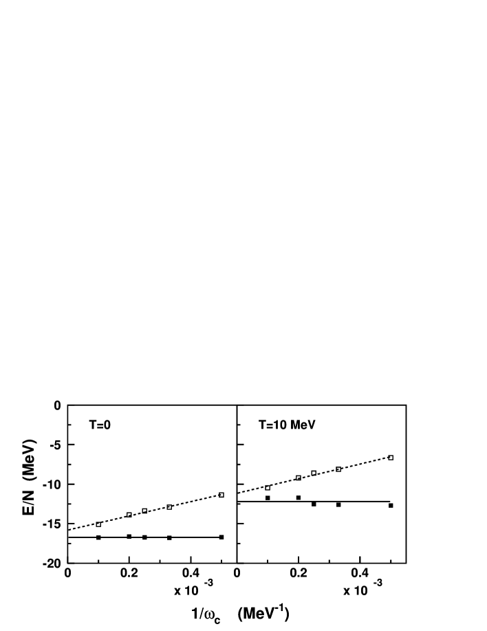
Figure 2: Internal energy per particle as a function of the cutoff at $T=0$ and $T=10\,\mbox{MeV}$. The dashed lines represent the energy calculated from the sum rule (6), the solid lines the energy from the summation of diagrams.

The result from the diagram summation can be compared to Galitskii-Koltun’s sum rule result extrapolated to infinite energy range (Table 1). This extrapolated value will be used in the following.

3.2 Pressure

The pressure is related to the thermodynamical potential through

$$\Omega(T,\mu,V)=-P\>\mathcal{V}\>.$$ (7)

It can be shown that

$$\Omega=-\mbox{Tr}\{\ln[G^{-1}]\}-\mbox{Tr}\{\Sigma G\}+\Phi\>.$$ (8)

The first two terms involve an integration over energy and momenta of single-particle propagators and self-energies. The calculation of the functional $\Phi$ requires instead a summation of a set of diagrams, evaluated in the following way. One notices that within the $T-$matrix approximation the diagrammatic expansions for the interaction energy and the functional $\Phi$ differ by the factor $1/n$ where $n$ is the number of interaction lines in the diagram . Hence the functional $\Phi$ can be obtained from the formula for the interaction energy

$$\Phi=\int_{0}^{1}\frac{d\lambda}{\lambda}<H_{pot}(\lambda V,G_{\lambda=1})>\ \ .$$ (9)

In the above formula the interaction potential is multiplied by the factor $\lambda$ but the propagator $G$ is the dressed nucleon propagator corresponding to the system with the full strength of interactions $(\lambda=1)$.

$\;T\;$	$\;E_{GK}/N\;$	$\;E_{diag}/N\;$	$\;P_{tot}/\rho\;$	$\;P_{BF}/\rho\;$
$0$	$-15.80$	$-16.63$	$-7.69$	$-5.58$
$2$	$-15.15$	$-16.29$	$-5.86$	$-5.4$
$5$	$-14.40$	$-15.24$	$-5.48$	$-5.2$
$10$	$-11.15$	$-11.72$	$-2.66$	$-3.35$
$20$	$-1.29$	$-1.21$	$\>\>6.49$	$4.74$

Table 1: Results (at $\rho=\rho_{0}$) of the internal energy and the pressure at zero and finite temperature (all values in MeVs). The second and third colum represent the internal energy per particle obtained from the Galitskii-Koltun’s sum rule (6) and from the diagram summation (3). The other columns contain our estimate for the pressure (from eq. (7)) and the results of Baldo and Ferreira [15].

The pressure in hot nuclear matter has been obtained using two-body Argonne $v_{14}$ interaction in the Bloch-De Dominicis approach [15]. The results are qualitatively similar, with a negative value of the pressure at $T=0$ and $\rho\simeq 0.16$ fm^-3. This shows the need to include three-body forces for a reliable description of the thermodynamics of the nuclear matter.

3.3 Entropy

We compute the entropy through the thermodynamic relation

$$\frac{S}{N}=\frac{1}{T}\left[\frac{E}{N}+\frac{P_{tot}}{\rho}-\mu\right]\>.$$ (10)

The results are plotted in Fig. 3. The error in the calculation of $TS$ at each temperature can be estimated by comparing the results obtained with the two expressions for the internal energy (3) and (6). The difference is of the order of $1$ MeV, also at zero temperature we find $|TS|\simeq 1\,\mbox{MeV}\neq 0$. The entropy can be estimated reliably only for $T\geq 5$ MeV, with the uncertainty shown as the hatched band in the figure.

We compare these results with other methods of calculating the entropy:

1. The dynamical quasiparticle formula [16]

   $$\displaystyle\frac{S_{DQ}}{N}=\frac{1}{\rho}\int\frac{d^{3}p}{(2\pi)^{3}}\frac{d\omega}{2\pi}\sigma(\omega)\left[A({\bf p},\omega)\left(1-\frac{\partial\mbox{Re}\Sigma^{R}(\mathbf{p},\omega)}{\partial\omega}\right)\right.$$

   $$+\displaystyle\left.\frac{\partial\mbox{Re}G^{R}(\mathbf{p},\omega)}{\partial\omega}\Gamma(\mathbf{p},\omega)\right]\ \ ,$$ (11)

   where

   $$\sigma(\omega)=-f(\omega)\ln[f(\omega)]-[1-f(\omega)]\ln[1-f(\omega)]\>.$$ (12)

   It has been shown that this one-body formula gives results close to the complete expression for the entropy [17].

2. The entropy calculated as for a free Fermi gas but using the effective mass $m^{*}$ (determined at each temperature by ${(\partial{\omega}_{p}/\partial p^{2})}_{p=p_{F}}=1/2m^{\star}$) instead of the rest mass $m$

   $$\frac{S_{{free}^{\star}}}{N}=\frac{1}{\rho}\int\frac{d^{3}p}{(2\pi)^{3}}\ \sigma\left(\frac{p^{2}}{2m^{\star}}\right)\ \ .$$ (13)

Figure 3: Entropy per baryon as a function of the temperature. The hatched band denotes our estimate of the entropy. The solid line denotes the result for the free Fermi gas with the in-medium effective mass and the dashed line represents the result of [17] (Eq. 1).

The entropy estimated by means of (1) and (13) is shown in Fig. 3 with the dashed and solid line respectively. Remarkably, we find that the expression for the entropy of the free Fermi gas is very similar to the result of the full calculation for the interacting system, if the change of the effective mass in the system is taken into account. The last observation simplifies significantly the modeling of the evolution of protoneutron stars [18], since relations between the entropy per baryon and the temperature derived for a fermion gas can be used in hot nuclear matter. As observed in [17] the quasiparticle expression (1) for the entropy [16] follows closely the full result.

4 Summary

We investigate the properties of correlated nuclear matter up to $T=20$ MeV. We calculate the internal energy with different methods, through the Galitskii-Koltun’s sum rule and by summing the diagrams which contribute to the expectation value of the interaction energy. The two methods give similar results at all temperatures up to a difference of about $1$ MeV which can be attributed to numerical inaccuracies. The pressure is derived from the thermodynamic potential which is given by the generating functional $\Phi$. The diagrams contributing to $\Phi$ are calculated with an integration of the interaction energy over an artificial parameter $\lambda$ which multiplies the interaction lines, while keeping the propagators dressed as in the fully correlated system. We finally estimate the entropy and compare it to two expressions derived in the context of a quasiparticle gas, whose results turn out to be close to the full calculation.

Only a study which embodies three-nucleon interactions can be realistically compared to experimental data on the nuclear equation of state. Here all calculations are carried out at the empirical saturation density, but the present scheme can be applied to other densities and it is suitable for the inclusion of three-body forces or the study of asymmetric nuclear matter, which will be addressed in a future work.

References

- [1] G. Baym and L.P. Kadanoff, Phys. Rev. 124 287 (1961)
- [2] G. Baym, Phys. Rev. 127 1392 (1962)
- [3] N.M. Hugenholz and L. Van Hove, Physica 24 363 (1958)
- [4] J. M. Luttinger, Phys. Rev. 119 1151 (1960)
- [5] P. Bożek and P. Czerski, Acta Phys. Polon. B34 2759 (2003)
- [6] Y. Dewulf, W. H. Dickhoff, D. Van Neck, E. R. Stoddard and M. Waroquier, Phys. Rev. Lett. 90 152501 (2003)
- [7] A. Akmal, V. R. Pandharipande and D. G. Ravenhall, Phys. Rev. C58 1804 (1998)
- [8] M. Baldo, A. Fiasconaro, H. Q. Song, G. Giansiracusa and U. Lombardo, Phys. Rev. C65 017303 (2002)
- [9] V. Somà and P. Bożek, nucl-th/0604030 (2006)
- [10] P. Bożek, Phys. Rev. C65 054306 (2002)
- [11] V. M. Galitskii and A. B. Migdal, Zh. Eksp. Teor. Fiz. 34 139 (1958)
- [12] P. C. Martin and J. Schwinger, Phys. Rev. 115 1342 (1959)
- [13] D. S. Koltun, Phys. Rev. Lett. 28 182 (1972)
- [14] A. L. Fetter and J. D. Walecka, Quantum theory of many-particle systems, McGraw-Hill, New York (1971)
- [15] M. Baldo and L. S. Ferreira, Phys. Rev. C59 682 (1998)
- [16] G.M. Carneiro and C.J. Pethick, Phys. Rev. D11 1106 (1975)
- [17] A. Rios, A. Polls, A. Ramos, and H. Müther, nucl-th/0605080 (2006)
- [18] M. Prakash et al, Phys. Rept. 280 1 (1997)