Are there plasminos in superconductors?

Abstract

Hot and/or dense, normal-conducting systems of relativistic fermions exhibit a particular collective excitation, the so-called plasmino. We compute the one-loop self-energy, the dispersion relation and the spectral density for fermions interacting via attractive boson exchange. It is shown that plasminos also exist in superconductors.

I Introduction

In relativistic fermionic systems at high temperature and/or high density, there are two types of fermionic excitations. Besides the ordinary excitation branches of particles and antiparticles, there are additional collective excitations, the so-called plasmino and anti-plasmino Klimov:1981ka ; Weldon:1982bn . These branches have opposite chirality compared to the ordinary excitation branches Weldon:1982bn . They coincide with the normal fermionic branches for vanishing momenta. For large momenta, they approach the lightcone and their spectral strengths vanish exponentially. The plasmino (anti-plasmino) branch has a minimum (maximum) for small, non-zero momenta. These excitations have been extensively investigated for normal-conducting matter Pisarski:1993rf ; Braaten:1991dd ; Blaizot:1996pu ; Thoma:1997dk ; Braaten:1990it ; Braaten ; Schaefer:1998wd ; Weldon:1989ys ; Pisarski:1989wb ; Baym:1992eu ; Peshier:1998dy ; Blaizot:1993bb ; Peshier:1999dt ; Mustafa:2002pb ; Wang:2004tg ; Kitazawa:2005pp , for a review see, for instance, Ref. Bellac .

With the exception of heavy-ion collisions, in the laboratory it is hard to achieve sufficiently large temperatures and densities such that a relativistic description for fermions becomes necessary, even if they are as light as electrons. On the other hand, there is a plethora of astrophysical situations where fermions have to be treated relativistically. For instance, the core of compact stellar objects could be sufficiently dense to consist of deconfined quark matter. The quark Fermi energy is then of the order of $\mu\sim 500$ MeV. Thus, at least the light up and down quark flavors have to be considered as relativistic particles, since $m\sim 5$ MeV $\ll\mu$. However, quark matter in compact stellar objects, if sufficiently cold, is not a normal-conducting system, but a color superconductor Review ; Rischke:2003mt . In this paper, we therefore investigate whether the plasminos known from normal-conducting systems survive in a superconductor. This is a question of general interest, independent of the specific nature of the superconductor (i.e., ordinary, color, etc.). To our knowledge, this problem has not been considered previously, since electrons can to good approximation be considered as non-relativistic in the condensed-matter context, and plasminos are absent if the temperature is smaller than the mass (at least for zero chemical potential Baym:1992eu ). It is also possible to formulate our expectation regarding the existence of plasminos in superconductors: plasminos are low-momentum excitations which, for large chemical potential $\mu\gg p$, are buried deep down in the Fermi sea. On the other hand, superconductivity is a Fermi-surface phenomenon. We thus expect that superconductivity should not exert a destructive influence on the presence of the plasmino excitations. Nevertheless, it requires an explicit calculation to prove this, which is the purpose of the present paper. We shall see that our expectations regarding the existence of plasminos in superconductors are confirmed.

The outline of this paper is the following. In Sec. II, we consider a normal-conducting system consisting of massless fermions interacting via scalar and vector boson exchange. For the sake of simplicity, we restrict our consideration to zero temperature. This case has been studied before by Blaizot and Ollitrault in Ref. Blaizot:1993bb . We largely confirm their results and extend them by computing the spectral density. We then study a superconducting system in Sec. III. Section IV concludes this paper with a summary of our results.

Our units are $\hbar=c=k_{B}=1$ and the metric tensor is $g^{\mu\nu}={\rm diag}(+,-,-,-)$. Four-vectors are denoted by capital letters, $K\equiv(k_{0},\vec{k})$. Three-vectors have modulus $k\equiv|\vec{k}|$ and direction $\hat{k}\equiv\vec{k}/k$. Our computations are done in the imaginary-time formalism where space-time integrals are denoted as $\int_{X}\equiv\int^{1/T}_{0}d\tau\int_{V}\,d^{3}\vec{x}$, while energy-momentum sums are $\int_{K}\equiv T\sum_{n}\int d^{3}\vec{k}/(2\pi)^{3}$ with $n=0,\pm 1\pm 2,...$ labeling the Matsubara frequencies for bosons, $\omega^{b}_{n}=2n\pi T$, and fermions, $\omega^{f}_{n}=(2n+1)\pi T$, respectively.

II Normal-Conducting Fermions

In this section the dispersion relation and the spectral density of massless normal-conducting fermions is reviewed in the limit $T\rightarrow 0$ Blaizot:1993bb . We first investigate the case where the interaction between the fermions is mediated by scalar bosons and compute the one-loop fermion self-energy. We then use the Dyson-Schwinger equation for the fermion propagator to perform a resummation of the one-loop self-energy to all orders. From the thus obtained quasiparticle propagator we determine the dispersion relation and the spectral density. Finally, we conclude this section with a discussion of the case where the interaction is mediated by vector bosons. Note that this treatment is not fully self-consistent in the sense that we do not use the result for the resummed quasiparticle propagator to recompute the one-loop self-energy for an iteration of the above procedure. Moreover, we do not solve a Dyson-Schwinger equation for the scalar boson propagator, which would lead to the generation of a boson mass $\sim g\mu$.

II.1 Self-energy

The inverse propagator for massless non-interacting fermions can be written in the form

$$G_{0}^{-1}(P)=P\mskip-11.0mu/+\mu\gamma_{0}\equiv\gamma_{0}\sum_{e=\pm}G_{0,e}^{-1}(P)\,\Lambda^{e}_{\vec{p}}\;,$$ (1)

where we introduced the energy projectors

$$\Lambda^{\pm}_{\vec{p}}=\frac{1}{2}(1\pm\gamma_{0}\vec{\gamma}\cdot\hat{p})\;,$$ (2)

and the free inverse propagators for positive/negative-energy solutions

$$G_{0,\pm}^{-1}(P)\equiv p_{0}+\mu\mp p\;.$$ (3)

Equation (1) can be easily inverted to give

$$G_{0}(P)=\sum_{e=\pm}G_{0,e}(P)\,\Lambda^{e}_{\vec{p}}\,\gamma_{0}\;,$$ (4)

with $G_{0,\pm}(P)=1/(p_{0}+\mu\mp p)$.

For fermions interacting with scalar bosons, the interaction part of the Lagrangian is of Yukawa-type, ${\cal L}_{I}=g\bar{\psi}\psi\phi$. The (perturbative) one-loop self-energy has the form Kapusta

$$\Sigma(P)=-g^{2}\,T\sum\limits_{n}\int\frac{d^{3}\vec{k}}{(2\pi)^{3}}\,{\cal D}_{0}(K-P)\,G_{0}(K)\;.$$ (5)

We assume the boson to be massless as well, with propagator ${\cal D}_{0}(Q)=-1/Q^{2}$, thus there is no tadpole contribution to the fermion self-energy. Performing the sum over the Matsubara frequencies one obtains

$$\Sigma(P)=-g^{2}\int\frac{d^{3}\vec{k}}{(2\pi)^{3}}\frac{1}{2E_{b}}\sum_{e=\pm}\Lambda^{e}_{\vec{k}}\gamma_{0}\left[\frac{1-N^{e}_{F}(k)+N_{B}(E_{b})}{p_{0}+\mu-e(k+E_{b})}+\frac{N^{e}_{F}(k)+N_{B}(E_{b})}{p_{0}+\mu-e(k-E_{b})}\right]\;.$$ (6)

Here, $E_{b}=|\vec{k}-\vec{p}|$ is the energy of the exchanged boson, $N_{F}^{\pm}(E)=[e^{(E\mp\mu)/T}+1]^{-1}$ are the thermal distribution functions for fermions and antifermions, and $N_{B}(E)=(e^{E/T}-1)^{-1}$ is the corresponding one for bosons.

We now project onto the self-energies for positive/negative-energy solutions,

$$\Sigma_{\pm}(P)\equiv\frac{1}{2}\,{\rm Tr}\left[\Lambda_{\vec{p}}^{\pm}\,\gamma_{0}\,\Sigma(P)\right]\;,$$ (7)

and perform an analytic continuation, $p_{0}+\mu\rightarrow\omega+i\eta$, where $\omega$ is the (real-valued) fermion energy relative to the vacuum Blaizot:1993bb .

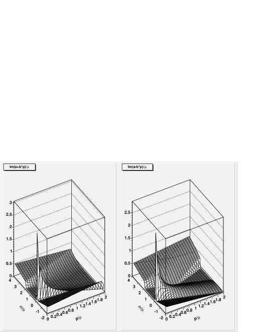
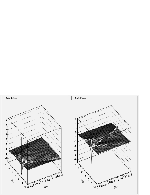
Figure 1: The imaginary parts of the self-energy for massless fermions (left panel) and antifermions (right panel) at $T=0$ and for an exemplary value of the coupling constant $g^{2}/(4\pi)=1$.

Figure 2: The real parts of the self-energy for massless fermions (left panel) and antifermions (right panel) at $T=0$ and for an exemplary value of the coupling constant $g^{2}/(4\pi)=1$.

Using Eq. (7), one readily calculates the imaginary part of the self-energy for positive/negative-energy solutions,

$$\hbox{Im}\,\Sigma_{\pm}(\omega,p)=\hbox{Im}\,a(\omega,p)\pm p\,\hbox{Im}\,b(\omega,p)\;.$$ (8)

Due to rotational invariance, the functions $\hbox{Im}\,a(\omega,p)$ and $\hbox{Im}\,b(\omega,p)$, which were first calculated in Ref. Blaizot:1993bb , only depend on the modulus of the momentum. For the sake of completeness we list the results in Appendix A. The real part of the self-energy for positive/negative-energy solutions is

$$\hbox{Re}\,\Sigma_{\pm}(\omega,p)=\hbox{Re}\,a(\omega,p)\pm p\,\hbox{Re}\,b(\omega,p)\;,$$ (9)

with the functions $\hbox{Re}\,a(\omega,p)$ and $\hbox{Re}\,b(\omega,p)$ given in Appendix A.

We show the functions (8) and (9) in Figs. 2 and 2, respectively. The shape of the imaginary and real parts reflect the different regions shown in Fig. 13. The peak of the imaginary parts in the region of low energies and momenta is due to the $1/p$ singularity of the function ${\rm Im}\,a$, cf. Eq. (36). The corresponding peak seen in the real parts, however, is due to the $1/p^{2}$ singularity of the function ${\rm Re}\,b$, cf. Eq. (42). This is the reason why the singularities appear with the same signs in the imaginary parts, but with opposite signs in the real parts of the self-energies for particles and antiparticles, cf. Eq. (7).

II.2 Dispersion relation

The full inverse fermion propagator is given by

$$G^{-1}(P)=G_{0}^{-1}(P)+\Sigma(P)\equiv\gamma_{0}\sum_{e=\pm}G_{e}^{-1}(P)\,\Lambda^{e}_{\vec{p}}\;,$$ (10)

where the full inverse propagator for positive/negative-energy solutions is

$$G_{\pm}^{-1}(P)\equiv G_{0,\pm}^{-1}(P)+\Sigma_{\pm}(P)\;.$$ (11)

The dispersion relations $p_{0}+\mu\equiv\omega=\omega_{\pm}^{*}(p)$ are given by the roots of the real parts of the inverse propagators,

$${\rm Re}\;G_{\pm}^{-1}(\omega_{\pm}^{*},p)=0\;.$$ (12)

We show the solutions of these equations in Fig. 3. The ordinary particle and antiparticle excitations correspond to the uppermost and lowermost curve, respectively. Besides these, for low momenta we find two additional roots of both Eqs. (12). The two solutions in the time-like region belong to the plasmino and antiplasmino branches. For massless particles right(left)-handedness implies positive (negative) helicity, while for massless antiparticles right(left)-handedness implies negative (positive) helicity. Since plasminos have opposite chirality from particles, the plasmino solution is actually a root of $G_{-}^{-1}=0$, while the antiplasmino is a root of $G_{+}^{-1}=0$. This also holds for the two additional solutions in the space-like region. However, since the imaginary parts for particles and antiparticles are large in this region, these excitations are strongly damped and do not have appreciable spectral weight, cf. Fig. 4. The plasmino solutions approach the lightcone and can no longer be found numerically for large momenta. The size of the momentum region where plasminos are found depends on the value of the coupling constant. For decreasing coupling constant, this region shrinks.

Figure 3: Dispersion relations of fermions for $g^{2}/(4\pi)=1$ at zero temperature. The thin lines represent the lightcone.

II.3 Spectral density

The spectral density is determined from the relation Fetter+Walecka

$$\rho_{\pm}(\omega,p)=-\frac{1}{\pi}\,\hbox{Im}\,G_{\pm}(\omega,p)\;.$$ (13)

If the imaginary part of the self-energy vanishes (see region IV of Fig. 13), the spectral density is proportional to a $\delta$-function with support on the quasiparticle mass shell, $\omega=\omega^{*}_{\pm}(p)$,

$$\rho_{\pm}(\omega,p)=\sum_{\omega^{*}_{\pm}}\,Z_{\pm}(\omega^{*}_{\pm})\,\delta(\omega-\omega^{*}_{\pm})\;,\;\;\;\;Z_{\pm}(\omega^{*}_{\pm})=\left|\frac{\partial\,{\rm Re}\,G_{\pm}^{-1}(\omega,p)}{\partial\omega}\right|_{\omega=\omega^{*}_{\pm}}^{-1}\;,$$ (14)

which corresponds to an infinite lifetime of the associated quasiparticle. This is the case for the plasmino branch and that part of the particle excitation branch, that is shown in Fig. 3. (For larger momenta, the particle excitation branch enters region Ia of Fig. 13 where the imaginary part is non-zero and, consequently, the particle excitation becomes unstable.) On the other hand, a non-zero imaginary part gives rise to a non-zero width of the spectral density,

$$\rho_{\pm}(\omega,p)=\frac{1}{\pi}\,\frac{\hbox{Im}\,\Sigma_{\pm}(\omega,p)}{\left[G_{0,\pm}^{-1}(\omega,p)+\hbox{Re}\,\Sigma_{\pm}(\omega,p)\right]^{2}+\left[\hbox{Im}\,\Sigma_{\pm}(\omega,p)\right]^{2}}\;.$$ (15)

This leads to a finite quasiparticle lifetime which is inversely proportional to the width of the spectral density around the quasiparticle mass shell. This is the case for all other fermionic excitation branches which lie outside region IV of Fig. 13.

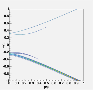
Figure 4: Contour plot of the spectral density of fermionic excitations in the limit of vanishing temperature and for $g^{2}/(4\pi)=1$.

In Fig. 4 we show the spectral density in a contour plot. Comparing this figure to Fig. 3, one can easily distinguish the particle, plasmino, antiplasmino, and antiparticle branches (from top to bottom). As mentioned above, the two solutions in the space-like region do not have sufficiently large spectral weight to appear in the contour plot. In other words, the width of the spectral density at the respective mass shell is large and, consequently, these excitations are strongly damped. Note also that the spectral weight of the two plasmino branches rapidly decreases for larger momenta.

II.4 Fermions interacting via vector bosons

The self-energy for fermions interacting via vector boson exchange is

$$\Sigma_{\rm v}(P)=-g^{2}T\sum\limits_{n}\int\frac{d^{3}\vec{k}}{(2\pi)^{3}}\,{\cal D}_{\mu\nu}(K-P)\,\gamma^{\mu}\,G_{0}(K)\,\gamma^{\nu}\;.$$ (16)

For massless vector bosons, this is a gauge-dependent expression. One easily convinces oneself that, in Feynman gauge for the gauge boson propagator, $\Sigma_{\rm v}(P)=2\,\Sigma(P)$. It was shown in Ref. Blaizot:1993bb that the same result holds also in Coulomb gauge. Finally, in the hard-thermal-loop (HTL) and hard-dense-loop (HDL) limit Weldon:1982bn , i.e., for $T,\mu\gg p_{0},p$, the result is gauge-independent, and again we have $\Sigma_{\rm v}(P)=2\,\Sigma(P)$, provided one takes the HTL/HDL limit on both sides of this equation. Therefore, all these cases are covered by the above discussion for scalar boson exchange via rescaling the coupling constant, $g\rightarrow g/\sqrt{2}$.

III Superconducting Fermions

We now turn to the question whether there are plasminos in superconductors. Our rationale is the following. We take the superconducting ground state as a basis for our calculation. Then, the fermion in the loop in Eq. (5) is no longer represented by a free propagator, $G_{0}(P)$, but by a quasiparticle propagator appropriate for superconducting systems, ${\cal G}_{0}$. We compute the one-loop self-energy for quasiparticle excitations in the superconductor. Afterwards, we resum the one-loop self-energy via a Dyson-Schwinger equation to obtain the propagator for quasiparticles and charge-conjugate quasiparticles. The poles of the propagator determine the dispersion relation. Finally, we calculate the spectral density.

Note that this treatment is not fully self-consistent. As in the normal-conducting case, we do not use the resummed quasiparticle propagator to obtain a self-consistent result for the one-loop self-energy. Moreover, we do not solve a gap equation for the superconducting gap parameter. Rather, we shall use an exemplary constant value for the gap function of particles, $\phi_{+}(P)=0.25\,\mu$ and set the gap function for antiparticles to zero, $\phi_{-}(P)=0$. The assumption of a constant gap function is justified only for point-like four-fermion interactions as in e.g. the Nambu–Jona-Lasinio model. For a boson exchange interaction of non-zero range, the gap function does depend on energy and momentum. Setting the antiparticle gap to zero is justified only in weak coupling, because then the contribution of the antiparticle modes to the gap equation is negligible Pisarski:1999tv ; Pisarski:1999av . Since antiparticle modes live far from the Fermi surface, a non-zero value (of reasonable magnitude) for the antiparticle gap would only have a negligible influence on our results for the excitation spectrum and spectral density of antiparticles.

Finally, we also do not solve a Dyson-Schwinger equation for the scalar boson propagator which would give rise to a mass $\sim g\mu$. Nevertheless, we expect that the complications arising from a fully self-consistent treatment, including the energy-momentum dependence of the gap function and non-vanishing antiparticle gaps, will only lead to quantitative, but not qualitative, changes of our results concerning the existence of plasminos in superconductors.

Let us finally note that, in a superconductor, fermions carry a charge with respect to a local (gauge) symmetry. This symmetry is spontaneously broken by condensation of Cooper pairs. An implicit assumption of our approach is that interactions due to exchange of vector bosons of the gauge interaction are negligible as compared to scalar boson exchange, i.e., that the one-loop fermion self-energy is dominated by the scalar interaction. If the fermions do not carry any charge, we are strictly speaking not considering a superconductor but a superfluid.

III.1 Self-energy

If fermions interact via scalar boson exchange, and if we only allow for pairing in the even-parity channel, the quasiparticle propagator reads Pisarski:1999av ; Fugleberg:2002rk

$${\cal G}_{0}(P)=\sum\limits_{e=\pm}\frac{p_{0}-(\mu-ep)}{p_{0}^{2}-(\mu-ep)^{2}-|\phi_{e}(P)|^{2}}\,\Lambda^{e}_{\vec{p}}\,\gamma_{0}\;.$$ (17)

(Note that our ${\cal G}_{0}$ corresponds to $G^{+}$ in Ref. Pisarski:1999av .)

The analogue of Eq. (5) for the superconducting system now reads

$$\Sigma(P)=-g^{2}\,T\sum\limits_{n}\int\frac{d^{3}\vec{k}}{(2\pi)^{3}}\,{\cal D}_{0}(K-P)\,{\cal G}_{0}(K)\;.$$ (18)

We compute the Matsubara sum using the mixed representation for the boson propagator,

$${\cal D}_{0}(\tau,\vec{q})=\frac{1}{2E_{b}}\left\{[1+N_{B}(E_{b})]\,e^{-E_{b}\tau}+N_{B}(E_{b})\,e^{E_{b}\tau}\right\}\;,$$ (19)

as well as the quasifermion propagator,

$${\cal G}_{0}(\tau,\vec{k})=-\sum_{e=\pm}\left[(1-n_{F}^{e})\,\frac{\epsilon_{e}-(\mu-ek)}{2\,\epsilon_{e}}\,e^{-\epsilon_{e}\tau}+n_{F}^{e}\,\frac{\epsilon_{e}+(\mu-ek)}{2\,\epsilon_{e}}\,e^{\epsilon_{e}\tau}\right]\,\Lambda_{\vec{k}}^{e}\,\gamma_{0}\;,$$ (20)

where $\epsilon_{e}\equiv\sqrt{(\mu-ek)^{2}+|\phi_{e}|^{2}}$, $n_{F}^{e}\equiv[e^{\epsilon_{e}/T}+1]^{-1}$. At vanishing temperature, the self-energy then becomes

$$\Sigma(P)=-g^{2}\int\frac{d^{3}\vec{k}}{(2\pi)^{3}}\frac{1}{4E_{b}}\sum_{e=\pm}\Lambda_{\vec{k}}^{e}\gamma_{0}\,\left[\left(1-\frac{\mu-ek}{\epsilon_{e}}\right)\frac{1}{p_{0}-\epsilon_{e}-E_{b}}+\left(1+\frac{\mu-ek}{\epsilon_{e}}\right)\frac{1}{p_{0}+\epsilon_{e}+E_{b}}\right]\;.$$ (21)

We now project onto positive/negative-energy states according to Eq. (7). After analytic continuation, the results for the imaginary and the real part of the self-energy can again be written in the form of Eqs. (8), (9). The functions ${\rm Im}\,a(\omega,p)$, ${\rm Im}\,b(\omega,p)$ are available in closed form and are given in Appendix B. However, the real parts ${\rm Re}\,a(\omega,p)$, ${\rm Re}\,b(\omega,p)$ have to be computed numerically. The results are shown in Figs. 6 and 6.

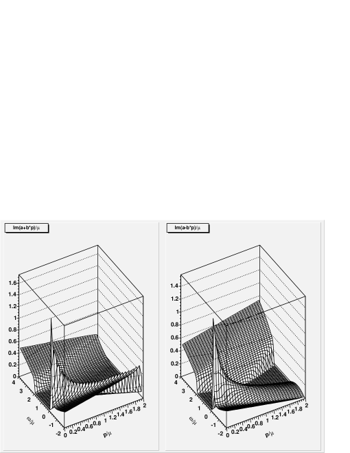
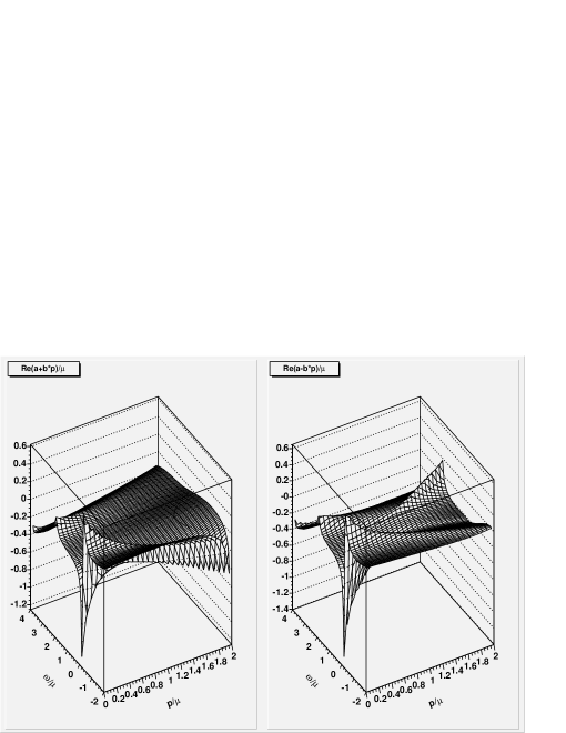
Figure 5: The imaginary parts of the self-energy for massless superconducting fermions (left panel) and antifermions (right panel), at $T=0$, for $\phi_{+}=0.25\,\mu$ and $\phi_{-}=0$.

Figure 6: The real parts of the self-energy for massless superconducting fermions (left panel) and antifermions (right panel), at $T=0$, for $\phi_{+}=0.25\,\mu$ and $\phi_{-}=0$.

Again, the shape of the imaginary and real parts reflects the different energy domains in Fig. 14, which are slightly different from those in Fig. 13. Apart from this, the overall shape is rather similar to that of the corresponding imaginary and real parts for normal-conducting fermions, cf. Figs. 2 and 2. Note, though, that the peaks are somewhat broader and flatter. This means that the damping of quasiparticles is larger than in the normal-conducting case.

III.2 Dispersion relation

We now compute the dispersion relation for superconducting fermions. As usual, it is advantageous to distinguish particles and charge-conjugate particles by introducing the Nambu-Gor’kov basis. The propagator for quasiparticles and charge-conjugate quasiparticles then reads, cf. Eq. (136) of Ref. Rischke:2003mt ,

$${\cal G}^{\pm}=\bigg{(}[G^{\pm}_{0}]^{-1}+\Sigma^{\pm}-\Phi^{\mp}\left\{[G^{\mp}_{0}]^{-1}+\Sigma^{\mp}\right\}^{-1}\Phi^{\pm}\bigg{)}^{-1}\;.$$ (22)

Here, the inverse free propagator for particles and charge-conjugate particles is

$$[G^{\pm}_{0}]^{-1}(P)=\gamma_{0}\sum\limits_{e=\pm}[p_{0}\pm(\mu-ep)]\Lambda^{\pm e}_{\vec{p}}\;.$$ (23)

Note that $G^{+}_{0}$ is identical with $G_{0}$ of Sec. II. Also, if we set $\Sigma^{\pm}\equiv 0$, ${\cal G}^{+}$ becomes identical with ${\cal G}_{0}$ in Eq. (17). Furthermore, the self-energy for particles, $\Sigma^{+}$, is the one we computed above, cf. Eq. (18). In the following, we only need its decomposition in terms of projections onto positive and negative energies,

$$\Sigma^{+}(P)=\gamma_{0}\sum_{e=\pm}\Sigma_{e}(P)\,\Lambda^{e}_{\vec{p}}\;.$$ (24)

The self-energy for charge-conjugate particles, $\Sigma^{-}$, can then be computed from $\Sigma^{+}$ via Rischke:2003mt

$$\Sigma^{-}(P)\equiv C\big{[}\Sigma^{+}(-P)\big{]}^{T}C^{-1}=-\gamma_{0}\sum_{e=\pm}\Sigma_{e}(-P)\,\Lambda^{-e}_{\vec{p}}\;,$$ (25)

where $C=i\gamma^{2}\gamma_{0}$ is the charge-conjugation matrix, and where we have used the identity $C\gamma_{\mu}C^{-1}=-\gamma_{\mu}^{T}$. Finally, $\Phi^{+}$ is the order parameter for condensation. If condensation occurs in the even-parity channel Pisarski:1999av ,

$$\Phi^{+}(P)=\sum\limits_{e=\pm}\phi_{e}(P)\,\Lambda^{e}_{\vec{p}}\,\gamma_{5}\;.$$ (26)

The charge-conjugate order parameter $\Phi^{-}$ is defined as

$$\Phi^{-}(P)\equiv\gamma_{0}\,\left[\Phi^{+}(P)\right]^{\dagger}\,\gamma_{0}=-\sum_{e=\pm}[\phi_{e}(P)]^{*}\,\Lambda^{-e}_{\vec{p}}\,\gamma_{5}\;.$$ (27)

The dispersion relation is given by the poles of the propagator (22). Inserting Eqs. (23) – (27) into Eq. (22), we obtain

$${\cal G}^{\pm}(P)=\left\{[G_{0}^{\mp}]^{-1}(P)+\Sigma^{\mp}(P)\right\}\sum\limits_{e=\pm}\Lambda^{\mp e}_{\vec{p}}\bigg{[}\bigg{(}p_{0}+\mu-ep+\Sigma_{e}(P)\bigg{)}\bigg{(}p_{0}-\mu+ep-\Sigma_{e}(-P)\bigg{)}-|\phi_{e}(P)|^{2}\bigg{]}^{-1}\;.$$ (28)

In order to see which poles belong to solutions for positive or negative energy, respectively, we perform the following projection of the quasiparticle propagator (28),

$${\cal G}^{\pm}_{e}(P)\equiv\frac{1}{2}\,{\rm Tr}\left[{\cal G}^{\pm}(P)\,\gamma_{0}\Lambda_{\vec{p}}^{e}\right]\;.$$ (29)

This gives

$${\cal G}^{+}_{+}(P) = \frac{p_{0}-\mu+p-\Sigma_{+}(-P)}{[p_{0}+\mu-p+\Sigma_{+}(P)][p_{0}-\mu+p-\Sigma_{+}(-P)]-|\phi_{+}(P)|^{2}}\;,$$ (30a)

$${\cal G}^{+}_{-}(P) = \frac{1}{p_{0}+\mu+p+\Sigma_{-}(P)}\;,$$ (30b)

$${\cal G}^{-}_{+}(P) = \frac{1}{p_{0}-\mu-p-\Sigma_{-}(-P)}\;,$$ (30c)

$${\cal G}^{-}_{-}(P) = \frac{p_{0}+\mu-p+\Sigma_{+}(P)}{[p_{0}+\mu-p+\Sigma_{+}(P)][p_{0}-\mu+p-\Sigma_{+}(-P)]-|\phi_{+}(P)|^{2}}\;.$$ (30d)

Since we have set $\phi_{-}=0$, there is a cancellation of terms between numerator and denominator in the propagators ${\cal G}_{-}^{+}$ and ${\cal G}_{+}^{-}$. This leads to a reduction in the number of poles.

Figure 7: Dispersion relations for superconducting fermions with positive energy for $T=0$, $g^{2}/(4\pi)=1$. The thin lines are the excitation branches for quasiparticles and quasiparticle-holes when setting $\Sigma^{+}=0$.

Figure 8: Dispersion relation for superconducting fermions with negative energy for $T=0$, $g^{2}/(4\pi)=1$. The thin lines are the excitation branches of normal antiparticles and antiparticle-holes.

After analytic continuation $p_{0}+\mu\rightarrow\omega+i\eta$, we obtain from the poles of ${\cal G}_{+}^{+}$ and ${\cal G}_{-}^{-}$ (these propagators have the same poles) the dispersion relation for particle, hole, antiplasmino, and antiplasmino-hole excitations (remember that the latter belong to the positive-energy part of the spectrum, and remember also that charge-conjugate anti-particles correspond to positive-energy solutions). These dispersion relations are shown in Fig. 8 for a value of the coupling constant $g^{2}/(4\pi)=1$. For comparison, the thin lines in this figure show the excitation branches of quasiparticles when setting $\Sigma^{+}\equiv 0$, i.e., the poles of the propagator (17) for the upper choice of signs. As seen in the normal-conducting case, Fig. 3, there were additional collective excitations in the space-like domain. We also find the corresponding excitations (plus their hole counterparts) in the superconducting case. These excitations do not have an appreciable spectral density (see below), they are strongly damped. The gap in the excitation spectrum is clearly visible. However, compared to the gap $2\,\phi_{+}=0.5\,\mu$ in the case $\Sigma^{+}=0$ (thin lines), it is shifted with respect to the Fermi surface $p=\mu$ to smaller values of momentum. This effective shift of the Fermi surface is well-known from Fermi-liquid theory and decreases with the coupling constant $g$.

From the poles of ${\cal G}^{+}_{-}$ we obtain the dispersion relation of antiparticle and plasmino excitations (as well as that of the additional excitation), while the poles of ${\cal G}^{-}_{+}$ correspond to plasmino-hole and antiparticle-hole excitations (as well as to the additional excitation in the hole sector). These dispersion relations are shown in Fig. 8. For comparison, we show the excitation branches of normal antiparticles and antiparticle-holes. As in the normal-conducting case, plasmino excitations as well as the additional strongly damped ones exist only in a region of momenta smaller than the Fermi momentum. The size of this region shrinks with decreasing values of the coupling constant.

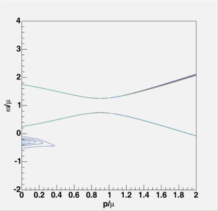
Figure 9: The spectral density $\rho_{+}^{+}$ for superconducting fermions, $T=0$, $g^{2}/(4\pi)=1$, $\phi_{+}=0.25\,\mu$, and $\phi_{-}=0$.

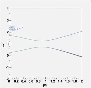
Figure 10: The spectral density $\rho_{-}^{-}$ for superconducting fermions, $T=0$, $g^{2}/(4\pi)=1$, $\phi_{+}=0.25\,\mu$, and $\phi_{-}=0$.

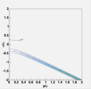
Figure 11: The spectral density $\rho^{+}_{-}$ for superconducting fermions, $T=0$, $g^{2}/(4\pi)=1$, $\phi_{+}=0.25\,\mu$, and $\phi_{-}=0$.

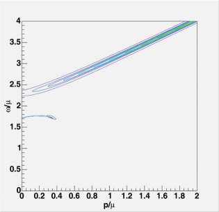
Figure 12: The spectral density $\rho^{-}_{+}$ for superconducting fermions, $T=0$, $g^{2}/(4\pi)=1$, $\phi_{+}=0.25\,\mu$, and $\phi_{-}=0$.

III.3 Spectral density

The spectral densities corresponding to the propagators (30) are computed via

$$\rho^{\pm}_{e}(\omega,p)=-\frac{1}{\pi}\,{\rm Im}\,{\cal G}^{\pm}_{e}(\omega,p)\;,$$ (31)

$e=\pm$. For the explicit calculation, see Appendix C.

In Fig.  12 we show a contour plot of $\rho^{+}_{+}$. For small momenta, the particle and hole branches are undamped, since in this region the imaginary part of the self-energy vanishes. Consequently, the spectral density is a delta function. For larger momenta, due to a non-zero imaginary part of $\Sigma_{+}$ the spectral density broadens on both the particle and the hole branch, however, for the particle branch this broadening is less pronounced than for the hole branch. One also observes the antiplasmino branch which is strongly damped by a non-zero imaginary part of the self-energy. Although the antiplasmino-hole branch corresponds to a pole of ${\cal G}^{+}_{+}$, it does not have appreciable spectral strength in $\rho^{+}_{+}$, due to a numerical cancellation of terms in the numerator of the expression for $\rho^{+}_{+}$, cf. Eq. (58).

In Fig. 12 we show the spectral density $\rho^{-}_{-}$. The spectral strength on the particle and hole branch is comparable to that for $\rho^{+}_{+}$. However, in contrast to that spectral density, now the antiplasmino-hole branch is clearly visible and the antiplasmino branch is suppressed due to a numerical cancellation of terms, cf. Eq. (61).

In Figs. 12 and 12 we show the spectral densities $\rho^{+}_{-}$ and $\rho^{-}_{+}$, respectively. We clearly distinguish the plasmino and antiparticle branches, as well as the corresponding hole excitations. The antiparticle and antiparticle-hole branches are strongly damped because of the non-vanishing imaginary part of the self-energy in this region of the energy-momentum plane. Note that results similar to ours have been obtained in Ref. Nickel:2006mm , applying the Maximum Entropy Method (MEM) to extract the spectral functions from Dyson-Schwinger equations.

IV Summary

In this work, we have studied the fermionic excitation spectrum in normal- and superconducting systems. For the sake of simplicity, we have taken the fermions to be massless and we have considered only the most simple case of an interaction mediated by massless scalar bosons. Moreover, we restricted our consideration to zero temperature. In normal-conducting, relativistic fermionic systems, there exist additional collective excitations, the so-called plasminos. These have opposite chirality compared to the usual particle excitations.

The goal of the present work was to investigate whether such excitations also exist in superconducting systems. In order to answer this question, we have first computed the one-loop fermion self-energy. Using this self-energy, we have determined the resulting dispersion relation from the poles of the full fermion propagator. We do indeed find plasmino excitations in superconducting systems.

In addition, we have also identified collective excitations which, at least for normal-conducting systems, lie in the space-like region of the energy-momentum plane. Both the plasmino and these additional collective excitations exist only in a region of low energies and momenta. We then calculated the spectral density and found that the additional collective excitations are strongly damped and do not carry appreciable spectral weight.

Appendix A Imaginary and real part of the self-energy of normal-conducting fermions

The imaginary and real part of the self-energy, see Eqs. (8) and (9), respectively, can be computed analytically. One distinguishes different regions in the energy-momentum plane as shown in Fig. 13. In these regions, the functions $\hbox{Im}\,a(\omega,p)$ and $\hbox{Im}\,b(\omega,p)$ assume the following values, see Ref. Blaizot:1993bb :

Figure 13: The different domains in the energy-momentum plane, which occur in the computation of the imaginary part of the self-energy.

$${\bf Ib:}\hskip 14.22636pt\hbox{Im}\,a(\omega,p) = \frac{g^{2}}{32\pi}\omega\;,$$ (32)

$$\hbox{Im}\,b(\omega,p) = -\frac{g^{2}}{32\pi}\;,\vspace*{1.0cm}$$ (33)

$${\bf Ia:}\hskip 14.22636pt\hbox{Im}\,a(\omega,p) = -\frac{g^{2}}{32\pi}\frac{1}{4p}(2\mu-\omega-p)(2\mu+\omega+p)\;,$$ (34)

$$\hbox{Im}\,b(\omega,p) = -\frac{g^{2}}{32\pi}\frac{1}{2p^{3}}(2\mu-\omega-p)\left[\omega^{2}-p^{2}-\frac{\omega}{2}(2\mu+\omega+p)\right]\;,\vspace*{1.0cm}$$ (35)

$${\bf II:}\hskip 14.22636pt\hbox{Im}\,a(\omega,p) = \frac{g^{2}}{32\pi}\frac{1}{4p}(2\mu-\omega-p)(2\mu+\omega+p)\;,$$ (36)

$$\hbox{Im}\,b(\omega,p) = \frac{g^{2}}{32\pi}\frac{1}{2p^{3}}(2\mu-\omega-p)\left[\omega^{2}-p^{2}-\frac{\omega}{2}(2\mu+\omega+p)\right]\;,\vspace*{1.0cm}$$ (37)

$${\bf III:}\hskip 14.22636pt\hbox{Im}\,a(\omega,p) = -\frac{g^{2}}{32\pi}\omega\;,$$ (38)

$$\hbox{Im}\,b(\omega,p) = \frac{g^{2}}{32\pi}\;,\vspace*{1.0cm}$$ (39)

$${\bf IV:}\hskip 14.22636pt\hbox{Im}\,a(\omega,p) = \hbox{Im}\,b(\omega,p)=0\;.$$ (40)

The real part of the self-energy is the sum of a vacuum and a matter contribution. After renormalization one obtains at the renormalization scale $\mu$ the result:

$$\hbox{Re}\,a(\omega,\vec{p}) = -\frac{g^{2}}{32\pi^{2}}\Biggl{\{}\mu+\frac{(2\mu-\omega-p)(2\mu+\omega+p)}{4p}\ln\Bigg{|}\frac{\omega+p}{\omega+p-2\mu}\Bigg{|}$$ (41)

$$\hskip 46.94704pt-\,\frac{(2\mu-\omega+p)(2\mu+\omega-p)}{4p}\ln\Bigg{|}\frac{\omega-p}{\omega-p-2\mu}\Bigg{|}+\omega\ln\Bigg{|}\frac{\omega^{2}-p^{2}}{\mu^{2}}\Bigg{|}\Biggr{\}}$$

$$\hbox{Re}\,b(\omega,\vec{p}) = -\frac{g^{2}}{16\pi^{2}}\Biggl{\{}\frac{\mu^{2}}{p^{2}}-\frac{\omega\mu}{2p^{2}}$$ (42)

$$\hskip 42.67912pt+\frac{(2\mu-\omega-p)}{4p^{3}}\left[\omega^{2}-p^{2}-\frac{\omega}{2}(2\mu+\omega+p)\right]\ln\Bigg{|}\frac{\omega+p}{\omega+p-2\mu}\Bigg{|}$$

$$\hskip 42.67912pt-\frac{(2\mu-\omega+p)}{4p^{3}}\left[\omega^{2}-p^{2}-\frac{\omega}{2}(2\mu+\omega-p)\right]\ln\Bigg{|}\frac{\omega-p}{\omega-p-2\mu}\Bigg{|}$$

$$\hskip 42.67912pt-\frac{1}{2}\ln\Bigg{|}\frac{\omega^{2}-p^{2}}{\mu^{2}}\Bigg{|}\Biggr{\}}\;.$$

Comparing this to Eq. (B6) of Ref. Blaizot:1993bb , we obtain an additional term $-\omega\mu/(2p^{2})$ in Eq. (42).

Appendix B Imaginary part of the self-energy of superconducting fermions

Superconductivity is a consequence of the formation of Cooper pairs at the Fermi surface, i.e., it involves particles, but not antiparticles. Therefore, it is permissible to set the antiparticle gap function to zero, $\phi_{-}(P)=0$. In the following, we abbreviate the particle gap function as $\phi_{+}(P)\equiv\phi$. The fact that particles have a gap but antiparticles do not forces us to compute particle and antiparticle contributions to the imaginary part of the self-energy (21) separately. We therefore split the latter into two parts. Using the projection (7), we obtain

$${\rm Im}\,\Sigma_{\pm}(\omega,p) = \sum_{e=\pm}{\rm Im}\,\Sigma_{\pm}^{(e)}(\omega,p)\;,$$ (43)

$${\rm Im}\,\Sigma_{\pm}^{(e)}(\omega,p) = {\rm Im}\,a^{(e)}(\omega,p)\pm p\,{\rm Im}\,b^{(e)}(\omega,p)\;,$$ (44)

$${\rm Im}\,a^{(e)}(\omega,p) = \pi\,g^{2}\,\int\frac{d^{3}\vec{k}}{(2\pi)^{3}}\frac{1}{8E_{b}}\,\left[\left(1-\frac{\mu-ek}{\epsilon_{e}}\right)\delta(p_{0}-\epsilon_{e}-E_{b})+\left(1+\frac{\mu-ek}{\epsilon_{e}}\right)\delta(p_{0}+\epsilon_{e}+E_{b})\right]\;,$$ (45)

$$p\,{\rm Im}\,b^{(e)}(\omega,p) = -\,e\pi\,g^{2}\,\int\frac{d^{3}\vec{k}}{(2\pi)^{3}}\frac{\hat{p}\cdot\hat{k}}{8E_{b}}\,\left[\left(1-\frac{\mu-ek}{\epsilon_{e}}\right)\delta(p_{0}-\epsilon_{e}-E_{b})+\left(1+\frac{\mu-ek}{\epsilon_{e}}\right)\delta(p_{0}+\epsilon_{e}+E_{b})\right]\;.$$ (46)

As in the case of normal-conducting fermions, we encounter different regions in the energy-momentum plane when computing the functions ${\rm Im}\,a^{(e)}(\omega,p)$, ${\rm Im}\,b^{(e)}(\omega,p)$. For the negative-energy contribution $(e=-)$ to the self-energy (21), these regions look the same as in Fig. 13, because we have set the antiparticle gap to zero. However, for the positive-energy contribution $(e=+)$, they are of slightly different shape due to the non-zero value for the particle gap $\phi$. We show these regions in Fig. 14.

In the following, we list the functions ${\rm Im}\,a^{(\pm)}(\omega,p)$, ${\rm Im}\,b^{(\pm)}(\omega,p)$ in the different domains of Fig. 14.

$$\textrm{\bf Ib:}\;\;\;{\rm Im}\,a^{(+)} = \frac{g^{2}}{32\pi}\omega\left[1-\frac{\phi^{2}}{2\omega p}\ln\left(\frac{\omega+p-2\mu}{\omega-p-2\mu}\right)\right]\;,$$ (47)

$${\rm Im}\,b^{(+)} = -\frac{g^{2}}{32\pi}\left\{1-\frac{\phi^{2}}{p^{2}}\left[1-\frac{\omega-2\mu}{2p}\ln\left(\frac{\omega+p-2\mu}{\omega-p-2\mu}\right)\right]\right\}\;,$$ (48)

$$\textrm{\bf Ia:}\;\;\;{\rm Im}\,a^{(+)} = -\frac{g^{2}}{32\pi}\frac{1}{4p}\left\{\left(2\mu-\omega-p\right)\left(2\mu+\omega+p\right)+\phi^{2}\left[\frac{4\mu}{\omega-p}+\frac{\phi^{2}}{(\omega-p)^{2}}+2\ln\left(\frac{(\omega-p)(\omega+p-2\mu)}{\phi^{2}}\right)\right]\right\}\;,\;\;\;\;\;\;\;\;$$ (49)

$${\rm Im}\,b^{(+)} = -\frac{g^{2}}{32\pi}\frac{1}{2p^{3}}\left\{\left(2\mu-\omega-p\right)\left[\omega^{2}-p^{2}-\frac{\omega}{2}\left(2\mu+\omega+p\right)\right]\right.$$ (50)

$$\hskip 56.9055pt+\frac{\phi^{2}}{\omega-p}\left[-2\mu p+\frac{\phi^{2}}{2}\frac{\omega-2p}{\omega-p}\right]\left.+\phi^{2}\left(\omega-2\mu\right)\ln\left(\frac{(\omega-p)(\omega+p-2\mu)}{\phi^{2}}\right)\right\}\;,$$

$$\textrm{\bf II:}\;\;\;{\rm Im}\,a^{(+)} = \frac{g^{2}}{32\pi}\frac{1}{4p}\left\{\left(2\mu-\omega-p\right)\left(2\mu+\omega+p\right)+\phi^{2}\left[\frac{4\mu}{\omega-p}+\frac{\phi^{2}}{(\omega-p)^{2}}+2\ln\left(\frac{(p-\omega)(2\mu-\omega-p)}{\phi^{2}}\right)\right]\right\}\;,\;\;\;\;\;\;$$ (51)

$${\rm Im}\,b^{(+)} = \frac{g^{2}}{32\pi}\frac{1}{2p^{3}}\left\{\left(2\mu-\omega-p\right)\left[\omega^{2}-p^{2}-\frac{\omega}{2}\left(2\mu+\omega+p\right)\right]\right.$$ (52)

$$\hskip 45.52458pt+\frac{\phi^{2}}{\omega-p}\left[-2\mu p+\frac{\phi^{2}}{2}\frac{\omega-2p}{\omega-p}\right]\left.+\phi^{2}\left(\omega-2\mu\right)\ln\left(\frac{(p-\omega)(2\mu-\omega-p)}{\phi^{2}}\right)\right\}\;,\;\;\;\;\;\;$$

$$\textrm{\bf III:}\;\;\;{\rm Im}\,a^{(+)} = -\frac{g^{2}}{32\pi}\phi^{2}\left[\frac{2\mu}{p^{2}-\omega^{2}}-\phi^{2}\frac{\omega}{(p^{2}-\omega^{2})^{2}}-\frac{1}{2p}\ln\left(\frac{\omega-p}{\omega+p}\right)\right]\;,$$ (53)

$${\rm Im}\,b^{(+)} = \frac{g^{2}\phi^{2}}{32\pi p^{2}}\left[1-\frac{2\mu\omega}{\omega^{2}-p^{2}}-\frac{\phi^{2}p^{2}}{(\omega^{2}-p^{2})^{2}}+\frac{2\mu-\omega}{2p}\ln\left(\frac{\omega+p}{\omega-p}\right)\right]\;,\;\;\;\;\;\;$$ (54)

$$\textrm{\bf IV:}\;\;\;{\rm Im}\,a^{(+)} = {\rm Im}\,b^{(+)}=0\;.$$ (55)

Figure 14: The different domains in the energy-momentum plane, which occur in the computation of the positive-energy contribution to the self-energy of superconducting fermions, shown for an exemplary value $\phi=0.25\,\mu$.

The negative-energy contribution to the self-energy vanishes except in region III of Fig. 13, where we find

$${\bf III:} \textrm{Im}\,a^{(-)}=-\frac{g^{2}}{32\pi}\omega$$ (57)

$$\textrm{Im}\,b^{(-)}=\frac{g^{2}}{32\pi}\;.$$

Appendix C Spectral density of superconducting fermions

The spectral densities for superconducting fermions are proportional to $\delta$-functions in the region of the energy-momentum plane, where the imaginary part of the self-energy is zero. In this case, they can be computed from an equation analogous to Eq. (14). On the other hand, if the imaginary part is non-zero, they can be computed via

$$\rho^{+}_{+}(\omega,p) = \frac{1}{\pi}\frac{1}{A^{2}+B^{2}}\Big{\{}\big{[}\omega-2\mu+p-{\rm Re}\Sigma_{+}(\mu-\omega,-\vec{p}\,)\big{]}\,B+{\rm Im}\Sigma_{+}(\mu-\omega,-\vec{p}\,)\,A\Big{\}}\,,$$ (58)

$$\rho^{+}_{-}(\omega,p) = \frac{1}{\pi}\frac{{\rm Im}\Sigma_{-}(\omega-\mu,\vec{p}\,)}{\left[\omega+p+{\rm Re}\Sigma_{-}(\omega-\mu,\vec{p}\,)\right]^{2}+\left[{\rm Im}\Sigma_{-}(\omega-\mu,\vec{p}\,)\right]^{2}}\,,$$ (59)

$$\rho^{-}_{+}(\omega,p) =- \frac{1}{\pi}\frac{{\rm Im}\Sigma_{-}(\mu-\omega,-\vec{p}\,)}{\left[\omega-2\mu-p-{\rm Re}\Sigma_{-}(\mu-\omega,-\vec{p}\,)\right]^{2}+\left[{\rm Im}\Sigma_{-}(\mu-\omega,-\vec{p}\,)\right]^{2}}\,,$$ (60)

$$\rho^{-}_{-}(\omega,p) = \frac{1}{\pi}\frac{1}{A^{2}+B^{2}}\Big{\{}\big{[}\omega-p+{\rm Re}\Sigma_{+}(\omega-\mu,\vec{p}\,)\big{]}\,B-{\rm Im}\Sigma_{+}(\omega-\mu,\vec{p}\,)\,A\Big{\}}\,,$$ (61)

where we have abbreviated

$$A = \left(\omega-\mu\right)^{2}-\big{(}\mu-p\big{)}^{2}+\big{(}\omega-2\mu+p\big{)}{\rm Re}\Sigma_{+}(\omega-\mu,\vec{p}\,)+\big{(}p-\omega\big{)}{\rm Re}\Sigma_{+}(\mu-\omega,-\vec{p}\,)$$ (62)

$$-{\rm Re}\Sigma_{+}(\omega-\mu,\vec{p}\,){\rm Re}\Sigma_{+}(\mu-\omega,-\vec{p}\,)+{\rm Im}\Sigma_{+}(\omega-\mu,\vec{p}\,){\rm Im}\Sigma_{+}(\mu-\omega,-\vec{p}\,)-\phi^{2}\,,\;\;\;\;\;$$

$$B = \big{(}\omega-2\mu+p\big{)}{\rm Im}\Sigma_{+}(\omega-\mu,\vec{p}\,)+\big{(}p-\omega\big{)}{\rm Im}\Sigma_{+}(\mu-\omega,-\vec{p}\,)$$ (63)

$$-{\rm Im}\Sigma_{+}(\omega-\mu,\vec{p}\,){\rm Re}\Sigma_{+}(\mu-\omega,-\vec{p}\,)-{\rm Re}\Sigma_{+}(\omega-\mu,\vec{p}\,){\rm Im}\Sigma_{+}(\mu-\omega,-\vec{p}\,).$$

References

- (1) V. V. Klimov, Sov. J. Nucl. Phys. 33 (1981) 934 [Yad. Fiz. 33 (1981) 1734]; Sov. Phys. JETP 55 (1982) 199 [Zh. Eksp. Teor. Fiz. 82 (1982) 336].
- (2) H. A. Weldon, Phys. Rev. D 26 (1982) 2789.
- (3) H. A. Weldon, Phys. Rev. D 40 (1989) 2410; Phys. Rev. D 61 (2000) 036003.
- (4) R. D. Pisarski, Nucl. Phys. A 498 (1989) 423C.
- (5) E. Braaten and R. D. Pisarski, Phys. Rev. D 42 (1990) 2156; Nucl. Phys. B 337 (1990) 569; Phys. Rev. Lett. 64 (1990) 1338; Phys. Rev. D 46 (1992) 1829; Phys. Rev. D 45 (1992) 1827.
- (6) E. Braaten and T. C. Yuan, Phys. Rev. Lett. 66 (1991) 2183.
- (7) E. Braaten, Astrophys. J. 392 (1992) 70.
- (8) G. Baym, J. P. Blaizot, and B. Svetitsky, Phys. Rev. D 46 (1992) 4043.
- (9) J. P. Blaizot and J. Y. Ollitrault, Phys. Rev. D 48 (1993) 1390.
- (10) R. D. Pisarski, Phys. Rev. D 47 (1993) 5589.
- (11) J. P. Blaizot, Nucl. Phys. A 606 (1996) 347.
- (12) M. H. Thoma and C. T. Traxler, Phys. Rev. D 56 (1997) 198.
- (13) A. Schaefer and M. H. Thoma, Phys. Lett. B 451 (1999) 195.
- (14) A. Peshier, K. Schertler, and M. H. Thoma, Annals Phys. 266 (1998) 162.
- (15) A. Peshier and M. H. Thoma, Phys. Rev. Lett. 84 (2000) 841.
- (16) M. G. Mustafa and M. H. Thoma, Pramana 60 (2003) 711.
- (17) S. Y. Wang, Phys. Rev. D 70 (2004) 065011.
- (18) M. Kitazawa, T. Kunihiro, and Y. Nemoto, Phys. Lett. B 631 (2005) 157.
- (19) M. Le Bellac, Thermal Field Theory (Cambridge University Press, Cambridge, 2000).
- (20) D. Bailin and A. Love, Phys. Rept. 107 (1984) 325; M. G. Alford, K. Rajagopal, and F. Wilczek, Phys. Lett. B 422 (1998) 247; R. Rapp, T. Schäfer, E. V. Shuryak, and M. Velkovsky, Phys. Rev. Lett. 81 (1998) 53; K. Rajagopal and F. Wilczek, arXiv:hep-ph/0011333; M. G. Alford, Ann. Rev. Nucl. Part. Sci. 51 (2001) 131;
- (21) D. H. Rischke, Prog. Part. Nucl. Phys. 52 (2004) 197.
- (22) J. I. Kapusta, Finite-temperature field theory (Cambridge University Press, Cambridge, 1993).
- (23) A. L. Fetter and J. D. Walecka, Quantum Theory of many-particle systems (McGraw-Hill Book Company, New York, 1971).
- (24) R. D. Pisarski and D. H. Rischke, Phys. Rev. D 61 (2000) 074017.
- (25) R. D. Pisarski and D. H. Rischke, Phys. Rev. D 60 (1999) 094013.
- (26) T. D. Fugleberg, Phys. Rev. D 67 (2003) 034013.
- (27) D. Nickel, [arXiv:hep-ph/0607224].