Antibound States and Halo Formation in the Gamow Shell Model

Abstract

The open quantum system formulation of the nuclear shell model, the so-called Gamow Shell Model (GSM), is a multi-configurational SM that employs a single-particle basis given by the Berggren ensemble consisting of Gamow states and the non-resonant continuum of scattering states. The GSM is of particular importance for weakly bound/unbound nuclear states where both many-body correlations and the coupling to decay channels are essential. In this context, we investigate the role of $\ell$=0 antibound (virtual) neutron single-particle states in the shell model description of loosely bound wave functions, such as the ground state wave function of a halo nucleus ¹¹Li.

I Introduction

The theoretical description of strongly correlated open quantum systems (OQS), such as the weakly bound/unbound atomic nuclei or atomic clusters, requires the rigorous treatment of both the many-body correlations and the continuum of positive-energy scattering states and decay channels (Dob98) ; (Oko03) . A major theoretical challenge is to consistently describe many-body states close to particle-emission thresholds where novel properties appear, such as, e.g., unusual radial features of halo states or threshold anomalies in the wave functions and associated observables. These features cannot be described in the closed quantum system (CQS) framework of a standard shell model (SM) which usually employs the single-particle (s.p.) basis of ${\cal L}^{2}$-functions of the harmonic oscillator. Representation of halo states in such a basis is not convenient. Moreover, the resonance and scattering states do not belong to the space of ${\cal L}^{2}$-functions.

The solution of the configuration interaction problem in the presence of continuum states (the so-called Continuum Shell Model) has been advanced recently in the OQS formulation of the nuclear SM, such as the Shell Model Embedded in the Continuum karim ; (Rot06) (real-energy continuum SM) and the Gamow Shell Model (GSM) (Mic02) ; (Mic03) ; (Bet02) ; (Bet03) ; (Mic04v1) ; (Rot06a) ; (Bet04) ; (Bet05) ; (Hag05) ; (Hag06) (SM in the complex $k$-plane). A variant of the real-energy continuum SM, based on the Feshbach projection formalism and phenomenological continuum-coupling, has been proposed in Ref. (Vol05) .

In the GSM, the multi-configurational SM is formulated in the rigged Hilbert space (Rig1) ; (Rig2) with a s.p. basis given by the Berggren ensemble (Ber68) ; (Ber93) consisting of Gamow (resonant or Siegert) states and the non-resonant continuum of scattering states. In general, resonant states correspond to the poles of the scattering matrix ($S$-matrix). These are the generalized eigenstates of the time-independent Schrödinger equation, which are regular at the origin and satisfy purely outgoing boundary conditions. The s.p. Berggren basis is generated by a finite-depth potential, and the many-body states are expanded in Slater determinants spanned by resonant and non-resonant s.p. basis states (Mic02) ; (Bet02) . The configuration mixing induced by the GSM Hamiltonian assures a simultaneous treatment of continuum effects and inter-nucleon correlations. Consequently, the GSM, which is a natural generalization of the SM for OQS, gives a natural description of many-body loosely bound and resonant states. In general, among different poles of the one-body $S$-matrix, one takes into account bound and decaying s.p. states to define the subset of resonant states in the Berggren ensemble. These poles, together with associated non-resonant continuum states, define the valence space. The actual selection of resonant states depends on the physical problem and on the convergence properties of resulting many-body GSM states.

An important question concerning the GSM deals with the inclusion of antibound (virtual) states in the Berggren ensemble. Antibound states have real and negative energy eigenvalues that are located in the second Riemann sheet of the complex energy plane (the corresponding momentum lies on the negative imaginary axis) (New66) ; (Nus72) ; (Tay72) ; (Dom81) . Contrary to bound states, the radial wave functions of virtual states increase exponentially at large distances. As often discussed in the literature, it is difficult to give a clear physical interpretation to virtual states. Strictly speaking, as the second energy sheet is considered unphysical and unaccessible through direct experiments, a virtual state is not a state but a feature of the system. If the virtual state has a sufficiently small energy, its presence has an appreciable influence on the behavior of the scattering cross section at low energies. Classic examples include the low-energy $1S_{0}$ nucleon-nucleon scattering characterized by a large and negative scattering length (Tay72) , scattering of slow electrons on molecules (Dub77) ; (Mor82) ; (Mor92) , and $eep$ Coulomb system (Tol97) . Related to this is an increased localization of real-energy scattering states just above threshold (Mig71) .

Coming back to nuclear structure, it was argued that the neutron-unbound ¹⁰Li nucleus sustains a low-lying $1s_{1/2}$ antibound state very close to the one-neutron (1n) emission threshold (Tho94) as a result of the inversion of $0p_{1/2}$ and $1s_{1/2}$ shells (Bro98) . Although many theoretical calculations predict the $0p_{1/2}-1s_{1/2}$ shell inversion, the phenomenon still remains a matter of debate Wur96 ; Des97 . Experimentally, several groups have reported evidence of the $\ell=0$ strength at the 1n-threshold in ¹⁰Li Shi97 ; Zin97 ; Shi98 ; You94 ; Kob93 ; (Zin95) ; however, no evidence of a weakly bound $1s_{1/2}$ state has been found. Since, experimentally, the n$+^{9}$Li has a large and negative scattering length, this may indicate the presence of the antibound $1s_{1/2}$ state in ¹⁰Li close to the 1n-threshold, though the presence of a low-lying $0p_{1/2}$ state cannot be ruled out (Boh97) .

The GSM calculations that explicitly consider the antibound $1s_{1/2}$ s.p. state (Bet04) ; (Bet05) were performed recently for the g.s. of ¹¹Li. The authors argued that the presence of an antibound state was important for the formation of a neutron halo. They have also noted that the bound state wave function of ¹¹Li could be expanded in terms of the real-energy, non-resonant $\ell$=0 continuum, i.e., without explicit inclusion of the antibound state. Moreover, a destructive interference between the $1s_{1/2}$ antibound s.p. state and the associated complex-energy, non-resonant $s_{1/2}$ background was noticed.

This work addresses the question of the $\ell$=0 virtual state for the description of a neutron halo by studying several complementary Berggren basis expansions and performing GSM calculations for ¹¹Li in different s.p. bases. In Sec. II, the one-body Berggren completeness relations with and without the $s_{1/2}$ antibound state are compared in the $\ell$=0 channel. Section III describes the g.s. of ¹¹Li in the schematic two-particle model using different s.p. Berggren ensembles, with and without the explicit inclusion of the antibound s.p. state $1s_{1/2}$. The comparison of convergence properties of the corresponding GSM calculations with the number of $s_{1/2}$ scattering states is made for the g.s. energy of ¹¹Li. A summary of results is given in Sec. IV.

II Completeness relations involving antibound $s_{1/2}$ states

One-body Berggren completeness relations with bound and resonant states have already been extensively studied for neutrons (Ber68) ; (Ber93) ; (BerLin93) ; (Lin93) ; (Mic03) and protons (Mic04v1) ; (Akram) . The standard Berggren completeness relation consists of a discrete sum over bound and resonant states, and an integral over non-resonant scattering states from the contour $L_{b}^{+}$ (see Fig. 1):

$$\sum_{n\in(b,d)}|u_{n}\rangle\langle u_{n}|+\int_{L_{b}^{+}}|u(k)\rangle\langle u(k)|\;dk=1,$$ (1)

where a discrete sum runs over all bound $(b)$ and resonant decaying $(d)$ states lying above the complex contour $L_{b}^{+}$. The continuous part takes into account the non-resonant scattering states lying on the contour. In the particular case of the $\ell$=0 neutron partial wave, there are no $s_{1/2}$ resonances due to the absence of both Coulomb and centrifugal barriers. Consequently, a real-$k$ contour would have been sufficient to describe the $s_{1/2}$ neutron channel. However, to investigate the convergence of imaginary part components of the expanded wave functions, we take the complex-$k$ contour $L_{b}^{+}$ close to the real-$k$ axis.

In this work, we shall perform detailed studies of the Berggren expansion in a more general case when an $\ell$=0 antibound s.p. state is included in the basis.

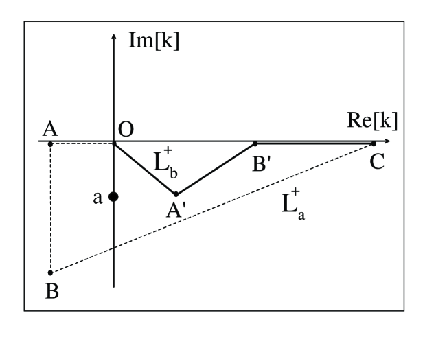
Figure 1: Contours in the complex-$k$ plane used in the Berggren completeness relations for the $s_{1/2}$ (Sec. II and Sec. III) and $p_{1/2}$ (Sec. III) partial waves. The $L^{+}_{a}$ contour (OABC) is only used in the $s_{1/2}$ channel; it allows wielding the antibound state $1s_{1/2}$ (marked as ‘a’). The $L^{+}_{b}$ contour (OA’B’C) is employed for $s_{1/2}$ and $p_{1/2}$ channels and permits expansions of bound and resonant states only.

In this case, the Berggren completeness relation takes the form (Lin93) ; (Bet04) :

$$\sum_{n\in(a,b,d)}|u_{n}\rangle\langle u_{n}|+\int_{L_{a}^{+}}|u(k)\rangle\langle u(k)|\;dk=1,$$ (2)

where the sum also includes antibound $(a)$ states lying above the complex contour $L_{a}^{+}$ (see Fig. 1). It is to be noted that, as discussed in Ref. (Lin93) , the contour $L_{a}^{+}$ is obtained by deforming continuously the contour $L_{b}^{+}$ placed in the fourth quadrant of the complex-$k$ plane so that it encompasses the antibound states of interest. In the unlikely situation that bound states of energies higher than antibound states $(a)$ are present, they must be excluded from the sum (2).

Bound states can be expanded with either of the completeness relations (1) or (2) , whereas antibound states can only be expressed through the more general completeness relation (2). Indeed, only those poles of the $S$-matrix which are situated above the contour can be expanded using the Berggren basis (Ber68) ; (Lin93) . The contour in the non-resonant continuum is usually discretized with a finite number of points in order to construct the Hamiltonian matrix (see Ref. (Mic03) for details).

In this study, the s.p. states entering the completeness relations (2) and (1) have been generated using an auxiliary Woods-Saxon (WS) Hamiltonian:

$$\hat{h} = \frac{\hat{p}^{2}}{2m}-\frac{V_{0}}{1+\exp\left(\frac{r-R_{0}}{d}\right)},$$ (3)

where $m$ is the reduced mass of a neutron with respect to the ⁹Li core, $d$=0.65 fm, and $R_{0}$=2.7 fm. The depth of the WS potential, $V_{0}$=50.5, 52.5, and 60.5 MeV, was adjusted to yield the $1s_{1/2}$ eigenstate respectively antibound at $-$0.002955 MeV, loosely bound at $-$0.0329 MeV, and well bound at $-$1.0372 MeV. The corresponding WS potentials are denoted as $WS_{1}$, $WS_{2}$, and $WS_{3}$ in the following.

In order to test Berggren completeness relations (2) and (1), we expand the $1s_{1/2}$ eigenstate of a given WS potential in the basis generated by another WS potential (WS⁽⁰⁾) of different depth:

$$|1s_{1/2}\rangle=\sum_{n}c_{n}|u_{n}\rangle+\int_{L^{+}}c(k)|u(k)\rangle\;dk$$ (4)

where $n$ is running either over bound and antibound $|u_{n}\rangle$ basis states in (2) or over bound $|u_{n}\rangle$ basis states in (1), and $L^{+}$ is $L_{a}^{+}$ or $L_{b}^{+}$, respectively. All the combinations of potentials studied are listed in Table 1. The contours $L_{a}^{+}$ and $L_{b}^{+}$ used in this section are defined by vertices (all in fm^-1): $[O=(0.0,0.0);A=(-0.01,0);B=(-0.01,-i0.02);C=(3.5,0.0)]$ and $[O=(0.0,0.0);A^{\prime}=(0.1,-i0.01);B^{\prime}=(1.5,0.0);C=(3.5,0.0)]$, respectively.

Table 1: Set of different WS potentials and $1s_{1/2}$ states used in numerical tests of the Berggren completeness relation. The Berggren ensemble generated by a potential WS⁽⁰⁾ (second column) consists of the $0s_{1/2}$ bound s.p. state, the contour in the non-resonant continuum (third column), and - possibly - the $1s_{1/2}$ s.p. state (fourth column). ‘No pole’ denotes a situation where the virtual $1s_{1/2}$ state is not included in the basis. In all the cases, the expansion has been carried out for the loosely bound $1s_{1/2}$ s.p. state of $WS_{2}$.

Case	WS(0)	Contour	$1s_{1/2}$ (WS(0))
(i)	$WS_{1}$	$L_{a}^{+}$	Antibound
(ii)	$WS_{1}$	$L_{b}^{+}$	No pole
(iii)	$WS_{3}$	$L_{b}^{+}$	Well bound

To assess the quality of the Berggren expansion, we calculate the rms deviation from the exact $1s_{1/2}$ halo wave function $u_{WS_{2}}(r)$ of $WS_{2}$ obtained by a direct integration of the Schrödinger equation. The rms deviation is calculated separately for the real and imaginary parts,

$$\mbox{rms}(\mbox{Re}[u]) = \sqrt{\frac{1}{N}\sum_{i=1}^{N}\mbox{Re}^{2}[u_{WS_{2}}(r_{i})-u_{{\rm WS}^{(0)}}(r_{i})]},$$ (5)

$$\mbox{rms}(\mbox{Im}[u]) = \sqrt{\frac{1}{N}\sum_{i=1}^{N}\mbox{Im}^{2}[u_{{\rm WS}^{(0)}}(r_{i})]},$$ (6)

for $N$=512 equidistant points on the real $r$-axis in the interval from $r$=0 to $r$=15 fm. In Eqs. (5) and (6) $u_{{\rm WS}^{(0)}}(r)$ is the $1s_{1/2}$ halo wave function of $WS_{2}$ expanded in the basis WS⁽⁰⁾ of Table 1.

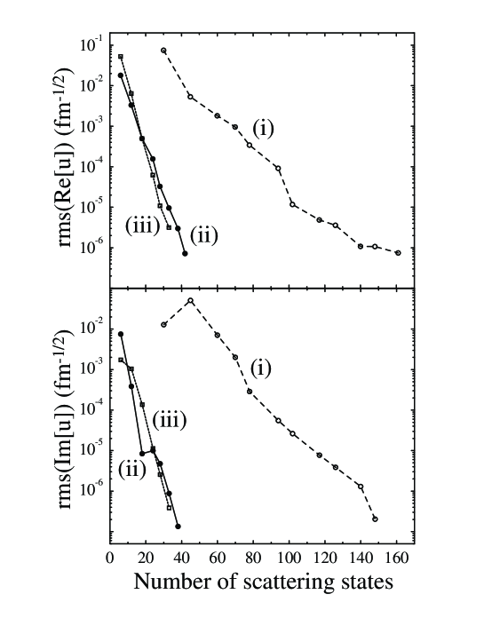
Figure 2: Real and imaginary parts of the rms deviations (5, 6) for the $1s_{1/2}$ halo wave function expanded in different Berggren bases as a function of the number of $s_{1/2}$ scattering wave functions on $L^{+}$. Cases (i)-(iii) of Table 1 are marked by dashed, solid, and dotted lines, respectively.

The calculated rms deviations (5) and (6) are shown in Fig. 2. One clearly sees that the Berggren basis containing an antibound state (case (i) in Table 1) is less efficient in expanding a loosely bound $1s_{1/2}$ state. The number of discretized scattering states in case (i) must be two-to-four times bigger than that in cases (ii) and (iii) in order to attain the same precision for the real part of the wave function. For the imaginary part, the difference is even more pronounced.

Without an antibound state in the basis, 40 to 50 non-resonant scattering states are enough to obtain the precision of order $10^{-6}$ for the calculated $s_{1/2}$ wave function, whereas 150 non-resonant scattering states are necessary to reach the same precision with this state included. In cases (ii) and (iii), one finds similar rms deviations, because the $s_{1/2}$ basis wave functions are in both cases either bound or close to the real (positive) $k$-axis; hence their contributions add up constructively. On the contrary, in case (i), the virtual state with exponentially increasing wave function interferes destructively with non-resonant scattering states in order to produce the halo state.

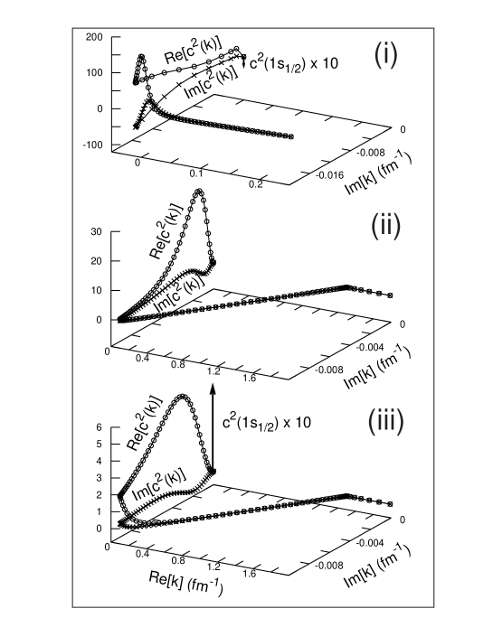
Figure 3: Real (circles) and imaginary (crosses) parts of the squared expansion amplitudes $c_{n}^{2}$ and $c^{2}(k)$ (4) corresponding to the Berggren bases (i-iii) of Table 1 in the complex $k$-plane for the $1s_{1/2}$ halo wave function. The amplitude $c^{2}_{0s_{1/2}}$ is practically negligible. In cases (i) and (iii), the amplitude $c_{1s_{1/2}}^{2}$ (magnified by a factor of 10) is represented by an arrow placed arbitrarily at $k$ = 0.

To illustrate this effect, Fig. 3 shows the distribution of squared amplitudes $c_{n}^{2}$ and $c^{2}(k)$ (4). By construction, the sum $\displaystyle\sum_{n}c_{n}^{2}+\int c^{2}(k)dk$ is always normalized to one. As the contribution from the $0s_{1/2}$ basis state is practically negligible, the set of $c_{n}^{2}$ reduces to the single real amplitude $c^{2}_{1s_{1/2}}$. In case (i), the non-resonant amplitudes $c^{2}(k)$ are much larger than their antibound counterpart $c_{1s_{1/2}}^{2}$, whereas in case (iii) the bound $1s_{1/2}$ pole carries half of the halo wave function. Case (ii) lies between these two extremes, as the halo state is built entirely from the non-resonant continuum but in an essentially coherent way (cf. Refs. (Bet04) ; (Mig71) ).

The results displayed in Fig. 3 demonstrate that the inclusion of the antibound pole in the basis enormously enhances the role of the non-resonant continuum which has to efface the incorrect asymptotics of an antibound pole in order to create a bound state with decaying asymptotics. This behavior is opposite to what is found when including a narrow resonant state in the Berggren ensemble. Such a state always concentrates a fairly large part of the expanded wave function (Mic03) ; (Mic04v1) .

III Contribution of antibound states to the two-body halo states: example of ¹¹Li

In order to assess the influence of antibound states on many-body halo states, we shall employ a schematic model (Bet04) ; (Bet05) of two valence particles, coupled to $J^{\pi}$=$0^{+}$, moving outside the inert core. In particular, we shall view the g.s. of ¹¹Li in terms of two neutrons in $s$ and $p$ angular momentum states coupled to the ⁹Li core. Our aim is not to exactly reproduce the structure of ¹¹Li but to learn how antibound s.p. states enter a two-body halo wave function.

The nuclear Hamiltonian is given by a WS potential representing a ⁹Li core, to which a Surface Gaussian Interaction (SGI) (Mic04v1) is added, modeling the residual interaction between the two valence nucleons:

$$\hat{H} = \sum_{i}\left[\frac{\hat{p}_{i}^{2}}{2m}-V_{0}\cdot f(r_{i})-4\;V_{so}\left(\vec{l_{i}}\cdot\vec{s_{i}}\right)\frac{1}{r_{i}}\left|\frac{df(r_{i})}{dr}\right|\right]$$ (7)

$$+ \sum_{i<j}V_{\rm SGI}\cdot\exp\left(-\left[\frac{\vec{r_{i}}-\vec{r_{j}}}{\mu}\right]^{2}\right)\cdot\delta(|\vec{r_{i}}|+|\vec{r_{j}}|-2R_{\rm SGI}).$$

Here, we employ the set of WS parameters $WS_{1}$ of Sec. II, and $V_{so}$=21.915 MeV is the strength of the spin-orbit potential. For these parameters, the $1s_{1/2}$ state is antibound and the $0p_{1/2}$ state is a resonance with the energy $E$=0.24 MeV and the width $\Gamma$=118 keV, in fair agreement with experimental data (Tho94) ; (Boh97) . The range of the residual SGI interaction is $\mu$=1  fm, $R_{\rm SGI}$=4.4 fm, and $V_{\rm SGI}$=$-1196$ MeV fm³. These parameters have been adjusted to reproduce the binding energy of ¹¹Li with respect to ⁹Li ($E_{B}$=–0.295 MeV), and a nearly 50% weight of the $s^{2}$ component, as suggested by the data (Tho94) .

The valence space consists of $s_{1/2}$, $p_{3/2}$, and $p_{1/2}$ neutron wave functions, from which the $0s_{1/2}$ and $0p_{3/2}$ bound states have been removed as they are part of the ⁹Li core. The $p_{3/2}$ s.p. space contains the $0p_{3/2}$ bound state pole and the real-energy $p_{3/2}$ contour with $k_{\rm max}$=2 fm^-1. The $p_{1/2}$ space consists of the $0p_{1/2}$ resonant pole and the $p_{1/2}$ contour of an $L_{b}^{+}$ type (see Fig. 1) defined by the vertices (all in fm^-1): $[O=(0.0,0.0);A^{\prime}=(0.1,-i0.1);B^{\prime}=(1.0,0.0);C=(2.0,0.0)]$. The $s_{1/2}$ space contains either a scattering component ($L_{b}^{+}$) or the $1s_{1/2}$ antibound pole to which the $s_{1/2}$ contour of an $L_{a}^{+}$-type is added. The contours $L_{a}^{+}$ and $L_{b}^{+}$ in the $s_{1/2}$ channel are defined by the vertices (all in fm^-1): $[O=(0.0,0.0);A=(-0.01,0);B=(-0.01,-i0.04);C=(2.0,0.0)]$ and $[O=(0.0,0.0);A^{\prime}=(0.1,-i0.01);B^{\prime}=(1.0,0.0);C=(2.0,0.0)]$, respectively. The $p_{3/2}$ and $p_{1/2}$ contours are discretized with 30 and 32 points, respectively. Each point represents one shell in GSM calculations. For this level of contour discretization and the momentum cut-off, the theoretical error on energies is about 1 keV for the real part and 0.01 keV for the imaginary part.

Table 2: Energy $E$ (in MeV) and width $\Gamma$ (in keV) of the ¹¹Li g.s. as a function of the number $N_{s_{1/2}}$ of the non-resonant scattering shells in the discretized $s_{1/2}$ continuum. The values of $E/\Gamma[L_{a}^{+}]$ (second and fourth columns) are calculated with the $s_{1/2}$ space consisting of the $1s_{1/2}$ antibound state and the associated $L_{a}^{+}$ $s_{1/2}$ contour. The values of $E/\Gamma[L_{b}^{+}]$ (third and fifth columns) are obtained with the $s_{1/2}$ space consisting of the $L_{b}^{+}$ $s_{1/2}$ contour only. See Fig. 1 for the definition of different contours.

$N_{s_{1/2}}$	$E[L_{a}^{+}]$	$E[L_{b}^{+}]$	$\Gamma[L_{a}^{+}]$	$\Gamma[L_{b}^{+}]$
10	–0.314	–0.291	65.274	–3.644
20	–0.292	–0.295	2.307	0.025
30	–0.294	–0.295	0.876	–0.003
40	–0.294	–0.295	–0.425	–0.007
50	–0.295	–0.295	0.075	–0.009
60	–0.295	–0.295	–0.005	–0.009

The convergence of the ¹¹Li g.s. energy as a function of the number of $s_{1/2}$ non-resonant scattering shells is shown in Table 2. The number of $s_{1/2}$ shells on each segment of the contours $L_{a}^{+}$ and $L_{b}^{+}$ is chosen so as to minimize a spurious width of the g.s. It is seen that the energy converges much faster when the antibound state is not present in the s.p. basis. In this case, the calculated g.s. energy of ¹¹Li attains a precision of 0.1 keV with 20 shells included, whereas as many as 50 shells are necessary to obtain the same level of precision if the antibound pole is present.

It is instructive to inspect the g.s. wave function of ¹¹Li expressed in different Berggren bases. Table 3 compares the GSM results obtained in the Berggren basis including the $1s_{1/2}$ antibound pole and $s_{1/2}$ non-resonant scattering states from the $L_{a}^{+}$ contour (case (i) of Table 1) with those obtained using the contour $L_{b}^{+}$ for the $s_{1/2}$ part (case (ii)). (The $p_{3/2}$ and $p_{1/2}$ spaces are defined as above.) To determine precisely the valence neutron configurations, 60 shells were taken along each of the scattering contours: $s_{1/2}$, $p_{1/2}$, and $p_{3/2}$. The expansion amplitudes of the $p$ components are identical in both cases and tote up to about 49%. As expected, important cancellations appear in case (i). Here, about 50% of the sum of squared amplitudes for configurations with two neutrons in $s_{1/2}$ non-resonant scattering states is cancelled by contributions from configurations involving one neutron in a scattering state and another one in the $1s_{1/2}$ antibound state. The antibound-antibound configuration $(1s_{1/2})^{2}$ contributes only $\sim$10%. In case (ii), however, all scattering two-neutron configurations add up coherently.

Table 3: Real and imaginary parts of squared amplitudes of the GSM configurations involving neutrons in $s_{1/2}$ orbits in the g.s. of ¹¹Li. The GSM calculations were performed using two Berggren bases: (a) including the $1s_{1/2}$ antibound pole state and the non-resonant scattering states $s_{1/2}$ along $L_{a}^{+}$ (second and fourth columns), and (b) including the non-resonant scattering states $s_{1/2}$ along $L_{b}^{+}$ (third and fifth columns). For the definition of contours, see Fig. 1.

Configuration	Re$[c^{2}]\{L_{a}^{+}\}$	Re$[c^{2}]\{L_{b}^{+}\}$	Im$[c^{2}]\{L_{a}^{+}\}$	Im$[c^{2}]\{L_{b}^{+}\}$
$(1s_{1/2})^{2}$	0.0990	–	–9.6033$\cdot 10^{-6}$	–
($1s_{1/2}$ $s_{1/2}$)	–0.5887	–	2.3369$\cdot 10^{-5}$	–
$(s_{1/2})^{2}$	1.0034	0.5137	–8.0720$\cdot 10^{-6}$	–1.4650$\cdot 10^{-5}$

IV Conclusions

The GSM has proven to be a powerful approach for the microscopic description of loosely bound and resonant states. The fact that the underlying Berggren basis directly incorporates one-particle continuum and the proper treatment of many-body correlations through configuration mixing makes it a perfect tool for a theoretical description of loosely bound many-body states such as nuclear halos.

In this study, we investigated the importance of including the virtual $\ell$=0 state in the s.p. basis for a modeling of one-body and two-body neutron halos. This question has experimental relevance: the data seem to suggest that the presence of the $s_{1/2}$ antibound state in ¹⁰Li is correlated with the appearance of the two-neutron halo in ¹¹Li.

Our calculation suggests that neither conceptual nor numerical gain is achieved if the antibound states are directly considered in the Berggren ensemble. In both one- and two-particle cases, it is always more advantageous to use a s.p. basis which contains non-resonant scattering states and, possibly, a bound $s_{1/2}$ pole. As the halo wave function has a decaying character at large distances due to the exponentially increasing asymptotics of the virtual state, its inclusion in the basis always induces strong negative interference with the scattering states. Therefore, adding antibound states to the basis is not beneficial, as more discretized scattering $s_{1/2}$ states are necessary to reach a required precision without providing any new information about the many-body wave function.

The use of antibound states in a Berggren basis can only be justified if the many-body state has a virtual character. This is certainly not the case for bound states, including halos. For instance, the g.s. halo in ¹¹Li is well described by using the Berggren basis solely involving the $s_{1/2}$ non-resonant scattering continuum and choosing the integration contour close to the real-$k$ axis. While the presence of an antibound state does require an increased density of discretized states around $k$=0, this can be handled efficiently by employing the density matrix renormalization group approach (Rot06a) . The resulting procedure yields much better numerical precision by suppressing the cancellations and leaving all the physical properties unchanged. Hence, the use of antibound states in GSM becomes questionable, as it worsens spurious effects due to continuum discretization.

- (1) J. Dobaczewski and W. Nazarewicz, Phil. Trans. R. Soc. Lond. A 356, 2007 (1998).
- (2) J. Okołowicz, M. Płoszajczak, and I. Rotter, Phys. Rep. 374, 271 (2003).
- (3) K. Bennaceur, F. Nowacki, J. Okołowicz, and M. Płoszajczak, Nucl. Phys. A 651, 289 (1999).
- (4) J. Rotureau, J. Okołowicz, and M. Płoszajczak, Nucl. Phys. A 767, 13 (2006).
- (5) N. Michel, W. Nazarewicz, M. Płoszajczak, and K. Bennaceur, Phys. Rev. Lett. 89, 042502 (2002).
- (6) N. Michel, W. Nazarewicz, M. Płoszajczak, and J. Okołowicz, Phys. Rev. C 67, 054311 (2003).
- (7) N. Michel, W. Nazarewicz, and M. Płoszajczak, Phys. Rev. C 70, 064313 (2004).
- (8) J. Rotureau, N. Michel, W. Nazarewicz, M. Płoszajczak, and J. Dukelsky, Phys. Rev. Lett, in press (2006); arXiv:nucl-th/0603021.
- (9) R. Id Betan, R. J. Liotta, N. Sandulescu, and T. Vertse, Phys. Rev. Lett. 89, 042501 (2002).
- (10) R. Id Betan, R. J. Liotta, N. Sandulescu, and T. Vertse, Phys. Rev. C 67, 014322 (2003).
- (11) R. Id. Betan, R. J. Liotta, N. Sandulescu, and T. Vertse, Phys. Lett. B 584, 48 (2004).
- (12) R. Id Betan, R. J. Liotta, N. Sandulescu, T. Vertse, and R. Wyss, Phys. Rev. C 72, 054322 (2005).
- (13) G. Hagen, M. Hjorth-Jensen, and J.S. Vaagen, Phys. Rev. C 71, 044314 (2005).
- (14) G. Hagen, M. Hjorth-Jensen, and N. Michel, Phys. Rev. C 73, 064307 (2006).
- (15) A. Volya and V. Zelevinsky, Phys. Rev. Lett. 94, 052501 (2005).
- (16) R. de la Madrid and M. Gadella, Am. J. Phys. 70, 626 (2002).
- (17) O. Civitarese and M. Gadella, Phys. Rep. 396, 41 (2004).
- (18) T. Berggren, Nucl. Phys. A 109, 265 (1968).
- (19) T. Berggren and P. Lind, Phys. Rev. C 47, 768 (1993).
- (20) R.G. Newton, Scattering Theory of Waves and Particles (McGraw-Hill, New York, 1966).
- (21) H.M. Nussenzveig, Causality and Dispersion Relations (Academic, New York, 1972).
- (22) J.R. Taylor, Scattering Theory (Wiley, New York, 1972).
- (23) W. Domcke, J. Phys. B 14, 4889 (1981).
- (24) L. Dubé and A. Herzenberg, Phys. Rev. Lett. 38, 820 (1977).
- (25) M.A. Morrison, Phys. Rev. A 25, 1445 (1982).
- (26) L.A. Morgan, Phys. Rev. Lett. 80, 1873 (1998).
- (27) O.I. Tolstikhin, V.N. Ostrovsky, and H. Nakamura, Phys. Rev. Lett. 79, 2026 (1997).
- (28) A.B. Migdal, A.M. Perelomov, and V.S. Popov, Yad. Fiz. 14, 874 (1971) (in Russian); Sov. J. Nucl. Phys 14, 488 (1972).
- (29) I.J. Thompson and M.V. Zhukov, Phys. Rev. C 49, 1904 (1994).
- (30) B.A. Brown, in Proceedings of the International School on Heavy Ion Physics, 4th Course: Exotic Nuclei, edited by R.A. Broglia and P.G. Hansen (World Scientific, Singapore, 1998), p.1.
- (31) J. Wurzer and H.M. Hofmann, Z. Phys. A 354, 135 (1996).
- (32) P. Descouvemont, Nucl. Phys. A 626, 647 (1997).
- (33) S. Shimoura et al., Nucl. Phys. A 616, 208c (1997).
- (34) M. Zinser et al., Nucl. Phys. A 619, 151 (1997).
- (35) S. Shimoura et al., Nucl. Phys. A 630, 387c (1998).
- (36) B.M. Young et al., Phys. Rev. C 49, 279,(1994).
- (37) T. Kobayashi, in Proceedings of Radioactive Nuclear Beams III, edited by D.J. Morrisey (Editions Frontiers, Gif-sur-Yvette, France, 1993) p. 169.
- (38) M. Zinser et al., Phys. Rev. Lett. 75, 1719 (1995).
- (39) H.G. Bohlen et al., Nucl. Phys. A 616, 254c (1997).
- (40) T. Berggren and P. Lind, Phys. Rev. C 47, 768 (1993).
- (41) P. Lind, Phys. Rev. C 47, 1903 (1993).
- (42) A.M. Mukhamedzhanov and M. Akin, arXiv:nucl-th/0602006.