Low-momentum interactions
with smooth cutoffs

Abstract

Nucleon-nucleon potentials evolved to low momentum, which show great promise in few- and many-body calculations, have generally been formulated with a sharp cutoff on relative momenta. However, a sharp cutoff has technical disadvantages and can cause convergence problems at the 10–100 keV level in the deuteron and triton. This motivates using smooth momentum-space regulators as an alternative. We generate low-momentum interactions with smooth cutoffs both through energy-independent renormalization group methods and using a multi-step process based on the Bloch-Horowitz approach. We find greatly improved convergence for calculations of the deuteron and triton binding energies in a harmonic oscillator basis compared to results with a sharp cutoff. Even a slight evolution of chiral effective field theory interactions to lower momenta is beneficial. The renormalization group preserves the long-range part of the interaction, and consequently the renormalization of long-range operators, such as the quadrupole moment, the radius and $\langle 1/r\rangle$, is small. This demonstrates that low-energy observables in the deuteron are reproduced without short-range correlations in the wave function.

1 Introduction

Internucleon potentials with variable momentum cutoffs, known generically as “$V_{{\rm low}\,k}$,” show great promise for few- and many-body calculations [1, 2, 3, 4, 5, 6, 7]. Changing the cutoff leaves observables unchanged by construction, but shifts contributions between the potential and the sums over intermediate states in loop integrals. These shifts can weaken or largely eliminate sources of non-perturbative behavior such as strong short-range repulsion or the tensor force [8]. An additional bonus is that the corresponding three-nucleon interactions become perturbative at lower cutoffs [4]. As a result, it is found in practice that few- and many-body calculations can be greatly simplified or converge more rapidly by lowering the cutoff. This has been observed with few-body variational methods [9, 10], the coupled-cluster approach [11], and for nuclear matter [5].

Low-momentum nucleon-nucleon interactions were originally derived and constructed in energy-independent form using model-space methods (such as Lee-Suzuki [1, 2] or Okubo [12]) applied in momentum space. These approaches define orthogonal subspaces with projection operators $P$ and $Q$, such that $P+Q=1$ and $PQ=QP=0$. In momentum space, the latter condition implies a sharp cutoff $\Lambda$ in (relative) momentum, so that $P$-space integrals run from 0 to $\Lambda$, while $Q$-space integrals run from $\Lambda$ to $\infty$ (or to a large “bare” cutoff). Subsequently, this $V_{{\rm low}\,k}$ construction was shown to be equivalent to a Renormalization Group (RG) treatment, derived by requiring cutoff independence of the half- or fully-on-shell $T$ matrix [3]. With a sharp cutoff, the equations take a particularly simple form and two-body observables are preserved for all momenta up to the cutoff.

However, a sharp cutoff also leads to cusp-like behavior for the interaction (close to the cutoff) in some channels and for the deuteron wave function, which becomes increasingly evident as the cutoff is lowered below $2\,\text{fm}^{-1}$. In some applications, this leads to slow convergence, for example at the 10–100 keV level in few-body calculations using harmonic oscillator bases (see Fig. 1). The reduction of the repulsive short-range interaction simultaneously reduces short-range correlations in the wave functions, which means that variational calculations can be effective with much simpler trial ansätze [9]. One would expect that such calculations for the deuteron and the triton, which are particularly low-energy bound states, should show improvement for cutoffs well below $2\,\text{fm}^{-1}$, but instead a degradation was observed in Ref. [9]. This result was attributed to the use of sharp cutoffs and a preliminary study [10] showed that these problems are alleviated by using a smooth-cutoff low-momentum interaction. In this paper, we verify this conclusion and explore in detail the construction and application of $V_{{\rm low}\,k}$ interactions with smooth cutoffs.

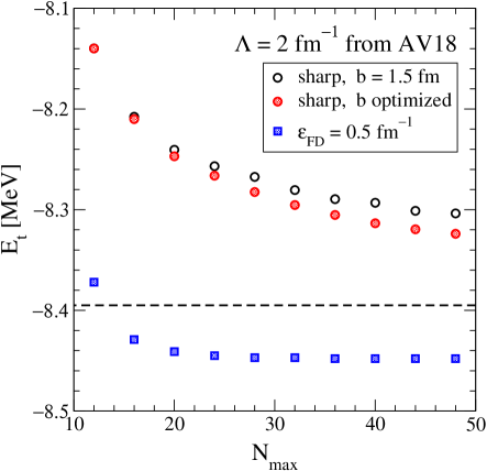
Figure 1: The triton binding energy $E_{t}$ calculated from a direct diagonalization in a harmonic oscillator basis of the low-momentum Hamiltonian derived from the Argonne $v_{18}$ potential [13] with cutoff $\Lambda=2\,\mbox{fm}^{-1}$, as a function of the size of the oscillator space ($N_{\rm max}\,\hbar\omega$ excitations). The open circles are calculated with a sharp cutoff for a fixed oscillator parameter $b$ while the filled ones correspond to optimizing $b$ at each $N_{\rm max}$. The dashed line indicates the exact Faddeev result using the sharp-cutoff interaction [4], and shows the slow convergence of the diagonalization at the 100 kev level. The squares are for a smooth Fermi-Dirac regulator, Eq. (32), that solves the convergence problem.

While smooth cutoffs seem incompatible with methods requiring $PQ=0$, it is not a conceptual problem for the RG approach. Indeed, there is an appreciable literature on smooth-cutoff regulators for applications of the functional or exact RG [14]. The functional RG keeps invariant the full generating functional, which translates into preserving all matrix elements of the inter-nucleon $T$ matrix. While this straightforwardly leads to RG equations, it also implies an energy-dependent interaction, which is undesirable for practical few- and many-body calculations. We resolve this conflict in Sect. 2 by constructing a low-momentum, energy-independent interaction with smooth cutoffs in three steps:

1. Evolve a large-cutoff potential to a lower, smooth cutoff while preserving the full off-shell $T$ matrix. This generates an energy-dependent low-momentum interaction.

2. Convert the energy dependence to momentum dependence, which results in a non-hermitian smooth-cutoff interaction.

3. Perform a similarity transformation to hermitize the low-momentum interaction.

Along with the possibility of many different functional forms for the smooth regulators, various hermitization schemes are possible, which reflects the general freedom in low-energy effective theories [15].

The freedom in defining low-energy potentials has consequences in practical calculations. This is already evident in Fig. 1, where the (converged) triton binding energy for a sharp cutoff is 50 keV less than for a particular Fermi-Dirac regulator. The difference reflects the different contribution from the (neglected) short-range three-body force. Just as changing a cutoff with a sharp regulator moves one along a Tjon line [4], we expect that changing the form of the regulator and the hermitization scheme at fixed cutoff also does. Thus, each combination of regulator (specified by one or more “sharpness” parameters) and hermitization scheme will have different corresponding three-body (and higher many-body) interactions.

In Sect. 3, we derive alternative energy-independent RG equations that are generalizations from sharp cutoffs. This approach has the advantage of a one-step construction, but accurate solutions of the resulting RG equations for low-momentum cutoffs are technically more challenging. The low-momentum interactions with smooth cutoffs, with different regulator types and different hermitization schemes, are applied in the two-body sector and to calculations of the triton in Sect. 4. We test the convergence properties and document the distortions of various combinations. In most cases we derive the low-momentum interactions starting from chiral effective field theory (EFT) potentials at N³LO [16, 17], but also use the Argonne $v_{18}$ potential [13] for comparison. We summarize our conclusions in Sect. 5 and give an outlook for future applications.

2 Smooth cutoff interactions via an energy-dependent RG

Our goal is to construct a smooth cutoff version of the energy-independent and hermitian low-momentum interaction $V_{{\rm low}\,k}$. In this section, we describe a three-step method that utilizes an energy-dependent RG equation to lower the cutoff, followed by two transformations that remove the energy dependence and the resulting non-hermiticity in the interaction. In the next section, we derive an equivalent method that uses a hermitian and energy-independent RG equation to construct the low-momentum interaction in one step.

First, we derive the RG equation for an energy-dependent low-momentum interaction $V_{\rm eff}(E)$, which is cut off by smooth regulators. It is convenient and efficient for numerical calculations to define the partial-wave interaction $V_{\rm eff}$ and the corresponding $T_{\rm eff}$ matrix in terms of a reduced potential $v$ and a reduced $t$ matrix as

$$V_{\rm eff}(k^{\prime},k;E) = f(k^{\prime})\,v(k^{\prime},k;E)\,f(k)\,,$$ (1)

$$T_{\rm eff}(k^{\prime},k;E) = f(k^{\prime})\,t(k^{\prime},k;E)\,f(k)\,,$$ (2)

where $f(k)$ is a smooth cutoff function satisfying

$$f(k)\stackrel{{\scriptstyle k\ll\Lambda}}{{\longrightarrow}}1\qquad\text{and}\qquad f(k)\stackrel{{\scriptstyle k\gg\Lambda}}{{\longrightarrow}}0\,.$$ (3)

The regulator functions are the same in each partial wave and possible choices are discussed in Sect. 4.

Given the low-momentum interaction $V_{\rm eff}(E)$, the reduced fully-off-shell $t$ matrix satisfies the Lippmann-Schwinger equation,

$$t(k^{\prime},k;E)=v(k^{\prime},k;E)+\frac{2}{\pi}\int_{0}^{\infty}p^{2}dp\,\frac{v(k^{\prime},p;E)\,f^{2}(p)\,t(p,k;E)}{E-p^{2}}\,,$$ (4)

where we use units with $\hbar=c=m=1$ and a principal value integral is implicit here and in the following. Note that the smooth cutoff is on the loop momentum but not on external momenta, and that $v$ and $f$ are cutoff dependent. We impose that the fully-off-shell $t(k^{\prime},k;E)$ is independent of the cutoff, $dt(k^{\prime},k;E)/d\Lambda=0$. This leads to an energy-dependent RG equation for the change in the reduced low-momentum interaction $v(k^{\prime},k;E)$ as the cutoff is lowered. In operator form, we have $t=v\,(1+G^{\Lambda}_{0}\,t)$ and thus $v=t\,(1+G^{\Lambda}_{0}\,t)^{-1}$. With $dU^{-1}=-U^{-1}\,dU\,U^{-1}$, we obtain (see also Ref. [18])

$$\frac{dv}{d\Lambda}=-t\,(1+G^{\Lambda}_{0}\,t)^{-1}\,\frac{dG^{\Lambda}_{0}}{d\Lambda}\,t\,(1+G^{\Lambda}_{0}\,t)^{-1}=-v\,\frac{dG^{\Lambda}_{0}}{d\Lambda}\,v\,.$$ (5)

Restoring the momentum and energy arguments, the energy-dependent RG equation reads

$$\frac{d}{d\Lambda}\,v(k^{\prime},k;E)=\frac{2}{\pi}\int_{0}^{\infty}p^{2}dp\,\frac{v(k^{\prime},p;E)\,\frac{d}{d\Lambda}[f^{2}(p)]\,v(p,k;E)}{p^{2}-E}\,.$$ (6)

For the implementation, we discretize the momentum space on a set of Gaussian mesh-points, which results in coupled RG equations that can be numerically integrated using standard methods. It is convenient to define discretized plane-wave states as $|\bar{k}\rangle\equiv k\sqrt{2w_{k}/\pi}\,|k\rangle$, where $w_{k}$ are the Gauss-Legendre weights. The new basis states are normalized as $\langle\bar{k}|\bar{p}\rangle=\delta_{k,p}$. Taking matrix elements of $v(E)$ between the discretized plane-wave states gives $v_{k^{\prime},k;E}\equiv\frac{2}{\pi}\,k^{\prime}k\sqrt{w_{k^{\prime}}w_{k}}\,v(k^{\prime},k;E)$, and Eq. (6) takes the simple matrix form

$$\frac{d}{d\Lambda}\,v_{k^{\prime},k;E}=\sum\limits_{p}\,v_{k^{\prime},p;E}\>\frac{\frac{d}{d\Lambda}[f^{2}_{p}]}{p^{2}-E}\>v_{p,k;E}\,.$$ (7)

Here and in the following, subscripts denote discrete momentum labels. In addition, it is convenient to convert the principal value integration to a normal integration using the standard principal-value subtraction method [19].

If we take a nucleon-nucleon (NN) potential model $V_{\rm NN}$ as the large-cutoff initial condition and numerically integrate the RG equation, the resulting energy-dependent $v(k^{\prime},k;E)$ preserves the fully-off-shell $T_{\rm NN}$ for all external momenta and energies, $t(k^{\prime},k;E)=T_{\rm NN}(k^{\prime},k;E)$. Therefore, $V_{\rm eff}(k^{\prime},k;E)=f(k^{\prime})\,v(k^{\prime},k;E)\,f(k)$ preserves the low momentum fully-off-shell $T_{\rm NN}$ matrix up to factors of the smooth cutoff function, $T_{\rm eff}(k^{\prime},k;E)=f(k^{\prime})\,T_{\rm NN}(k^{\prime},k;E)\,f(k)$.

In the second step, we convert the energy dependence of $V_{\rm eff}(E)$ to momentum dependence by using a method similar to field redefinitions. For this purpose, we introduce an energy-independent (but non-hermitian) $V_{{\rm low}\,k}(k^{\prime},k)$ that reproduces the half-on-shell $T_{\rm eff}$ matrix (and hence wave functions) as $V_{\rm eff}(k^{\prime},k;E)$,

$$\langle k^{\prime}|T_{\rm eff}(p^{2})|p\rangle=\langle k^{\prime}|V_{\rm eff}(p^{2})|\chi_{p}\rangle\equiv\langle k^{\prime}|V_{{\rm low}\,k}|\chi_{p}\rangle\,,$$ (8)

where $|\chi_{p}\rangle$ are the eigenstates of the energy-dependent Hamiltonian $H_{\rm eff}(p^{2})=T+V_{\rm eff}(p^{2})$ with relative kinetic energy $T$. Using the completeness of the interacting eigenstates, this leads to

$$V_{{\rm low}\,k}(k^{\prime},k)=\int_{0}^{\infty}p^{2}dp\>\frac{2}{\pi}\int_{0}^{\infty}p^{\prime 2}dp^{\prime}\,V_{\rm eff}(k^{\prime},p^{\prime};p^{2})\,\chi_{p}(p^{\prime})\,\widetilde{\chi}_{p}^{*}(k)\,.$$ (9)

The energy dependence of $H_{\rm eff}(p^{2})$ necessitates the use of bi-orthogonal complement vectors $\langle\widetilde{\chi}_{p}|$ in the completeness relation, $\int p^{2}dp\,|\chi_{p}\rangle\langle\widetilde{\chi}_{p}|=\leavevmode\hbox{\small 1\normalsize\kern-3.30002pt1}$. If bound states are present, the integral over the continuous scattering states includes a summation over bound states as well.

For the numerical solution of Eq. (9), we first obtain the eigenstates of the energy-dependent $H_{\rm eff}$ by self-consistently diagonalizing the discretized eigenvalue equation

$$\sum_{k}\bigl{(}\delta_{k^{\prime}k}\,k^{2}+V^{\rm eff}_{k^{\prime},k;E_{p}}\bigr{)}\chi_{k,p}=E_{p}\,\chi_{k^{\prime},p}\,.$$ (10)

Next, the discretized bi-orthogonal complement vectors are obtained from the matrix equation $\sum_{p}\chi_{k,p}\,\widetilde{\chi}_{k^{\prime},p}=\delta_{k,k^{\prime}}$. Finally, Eq. (9) is evaluated by simple matrix multiplication

$$V^{{\rm low}\,k}_{k^{\prime},k}=\sum\limits_{p,p^{\prime}}\,V^{\rm eff}_{k^{\prime},p^{\prime};E_{p}}\,\chi_{p^{\prime},p}\,\widetilde{\chi}_{k,p}\,.$$ (11)

This procedure is straightforward in practice. The only subtlety arises when the discretization of the defining equations for the bi-orthogonal complement vectors is such that some of the $|\chi_{p}\rangle$ vectors appear to be linearly dependent. In this case, singular-value-decomposition methods are helpful to solve the singular system of equations by setting to zero the problematic small singular values when taking the inverse of the $\chi_{k,p}$ matrix [19]. The resulting energy-independent $V_{{\rm low}\,k}$ is non-hermitian, and is identical to the solution of the energy-independent RG equation derived from half-on-shell $t$ matrix equivalence in the next section.

The method can be improved further by integrating the energy-dependent RG equation, Eq. (6), formally instead of a numerical integration. That is, using $dv^{-1}=-v^{-1}\,dv\,v^{-1}=dG^{\Lambda}_{0}$, we obtain $v^{-1}-V_{\rm NN}^{-1}=G^{\Lambda}_{0}-G_{0}$, and we recover the Bloch-Horowitz equation generalized to a smooth cutoff,

$$v(k^{\prime},k;E)=V_{\rm NN}(k^{\prime},k)+\frac{2}{\pi}\int_{0}^{\infty}p^{2}dp\,\frac{V_{\rm NN}(k^{\prime},p)\,[1-f^{2}(p)]\,v(p,k;E)}{E-p^{2}}\,.$$ (12)

Converting the RG equation to this integral equation and solving by matrix methods speeds up the calculation considerably and reduces the accumulation of numerical errors.

Finally, we note that the initial energy-dependent RG equation is not needed if one starts directly from the smooth-cutoff generalization of the Bloch-Horowitz equation. For this purpose, we separate the free two-nucleon propagator into a smooth-cutoff low-momentum $G^{\Lambda}_{0}$ and a high-momentum part $\overline{G^{\Lambda}_{0}}$. The Lippmann-Schwinger equation then reads $T_{\rm NN}(E)=V_{\rm NN}+V_{\rm NN}\,(G^{\Lambda}_{0}(E)+\overline{G^{\Lambda}_{0}}(E))\,T_{\rm NN}(E)$, and a rearrangement gives the fully-off-shell $T_{\rm NN}(E)$ matrix with only low-momentum propagators,

$$T_{\rm NN}(E)=v(E)+v(E)\,G^{\Lambda}_{0}(E)\,T_{\rm NN}(E)\,,$$ (13)

where $v(E)$ is the solution to the smooth-cutoff Bloch-Horowitz equation, Eq. (12).

2.1 Hermitian low-momentum interactions

In the third step, we remove the non-hermiticity of $V_{{\rm low}\,k}$ by a similarity transformation that orthogonalizes the set of eigenvectors $\{|\chi_{p}\rangle\}$ of the non-hermitian Hamiltonian $H_{{\rm low}\,k}=T+V_{{\rm low}\,k}$. Following Holt et al. [20], we define a transformation $Z$ by

$$Z|\chi_{p}\rangle=\,|\xi_{p}\rangle\qquad\text{and}\qquad\langle\xi_{p}|\xi_{p^{\prime}}\rangle=\delta_{pp^{\prime}}\,,$$ (14)

where the Kronecker delta normalization implies the discretization procedure of the previous section has been carried out. The hermitian low-momentum interaction is then given by

$$\overline{V}_{{\rm low}\,k}=Z\,H_{{\rm low}\,k}\,Z^{-1}-T\,.$$ (15)

There is not a unique choice for the transformation $Z$, which is a reflection of the general freedom in low-energy effective theories. In Ref. [20], it was shown how several common hermitization methods correspond to different choices for $Z$. For example, within the Lee-Suzuki framework [21, 22] for deriving effective interactions (which implies a sharp cutoff corresponding to orthogonal $PQ=0$ projection operators), the eigenstates of the non-hermitian $V_{{\rm low}\,k}$ obey

$$\langle\chi_{p}|P+\omega^{\dagger}\omega|\chi_{p^{\prime}}\rangle=\delta_{pp^{\prime}}\,,$$ (16)

where $\omega=Q\omega P$ is the wave operator that parameterizes the Lee-Suzuki decoupling transformation. Identifying $Z^{\dagger}Z=P+\omega^{\dagger}\omega$ defines a class of valid transformations for $Z$. For example, setting $Z=\sqrt{P+\omega^{\dagger}\omega}$ corresponds to the hermitization procedure of Okubo [23] and Okamoto and Suzuki [24]. Alternatively, one can perform a Cholesky factorization of the symmetric and positive-definite operator $LL^{\dagger}=P+\omega^{\dagger}\omega$, where $L$ is the lower-triangular Cholesky matrix. Then, $Z=L^{\dagger}$ corresponds to the hermitization method of Andreozzi [25]. Another method discussed by Holt et al. is a Gram-Schmidt orthogonalization to construct the set of $\{|\xi_{p}\rangle\}$ directly from $\{|\chi_{p}\rangle\}$. This allows $Z$ to be calculated directly from Eq. (14). Even within the Gram-Schmidt method, $Z$ is not unique, due to the freedom in choosing the starting vector. All hermitization methods result in low-momentum interactions $\overline{V}_{{\rm low}\,k}$ that preserve the low-momentum fully-on-shell $T_{\rm NN}$ matrix, up to factors of the regulator function $T_{{\rm low}\,k}(k,k;k^{2})=f^{2}(k)\,T_{\rm NN}(k,k;k^{2})$, and the deuteron binding energy. The corresponding three-body interactions will differ, however, as discussed below.

The Gram-Schmidt method can be applied directly to the smooth-cutoff $V_{{\rm low}\,k}$. As in Ref. [20], the orthogonal basis $\{|\xi_{p}\rangle\}$ is constructed via

$$|\xi_{1}\rangle = Z_{11}|\chi_{1}\rangle$$

$$|\xi_{2}\rangle = Z_{21}|\chi_{1}\rangle+Z_{22}|\chi_{2}\rangle$$ (17)

$$|\xi_{3}\rangle = Z_{31}|\chi_{1}\rangle+Z_{32}|\chi_{2}\rangle+Z_{33}|\chi_{3}\rangle$$

$$\vdots$$

where the $Z_{pp^{\prime}}$ are determined sequentially so that $\langle\xi_{p}^{\prime}|\xi_{p}\rangle=\delta_{pp^{\prime}}$. We have chosen to take the eigenstate of $H_{{\rm low}\,k}$ with lowest energy as the starting vector, although any other linear combination could have been used. In practice, the modified Gram-Schmidt algorithm with re-orthogonalization of Ref. [26] is utilized to guard against round-off errors. The transformation $Z$ corresponding to the Gram-Schmidt hermitization is then given by

$$Z=\sum_{p}|\xi_{p}\rangle\,\langle\widetilde{\chi}_{p}|\qquad\text{and}\qquad Z^{-1}=\sum_{p}|\chi_{p}\rangle\,\langle\xi_{p}|\,.$$ (18)

In contrast to the Gram-Schmidt method, the other hermitization schemes are formulated in terms of the Lee-Suzuki wave-operator $\omega$, which apparently relies on the use of orthogonal projection operators $PQ=0$ corresponding to sharp cutoffs. In order to generalize the Okubo and Andreozzi hermitization schemes to smooth cutoffs, it is necessary to eliminate all references to $\omega$. This is easily done by noting that the bi-orthogonal complement vectors are defined through $\langle\widetilde{\chi}_{p}|\chi_{p^{\prime}}\rangle=\delta_{pp^{\prime}}$. For a sharp cutoff, Eq. (16) implies $|\widetilde{\chi}_{p}\rangle=(P+\omega^{\dagger}\omega)|\chi_{p}\rangle$, and thus

$$P+\omega^{\dagger}\omega=\sum_{p}|\widetilde{\chi}_{p}\rangle\,\langle\widetilde{\chi}_{p}|\,.$$ (19)

For smooth cutoffs, the obvious generalization is to construct the operator $\sum_{p}|\widetilde{\chi}_{p}\rangle\,\langle\widetilde{\chi}_{p}|$ and decompose it as

$$Z^{\dagger}Z=\sum_{p}|\widetilde{\chi}_{p}\rangle\,\langle\widetilde{\chi}_{p}|\,.$$ (20)

As for sharp cutoffs, the generalized Okubo transformation corresponds to $Z=\sqrt{\sum_{p}|\widetilde{\chi}_{p}\rangle\,\langle\widetilde{\chi}_{p}|}$, where the square root is taken in the eigenbasis of the positive-definite operator $\sum_{p}|\widetilde{\chi}_{p}\rangle\,\langle\widetilde{\chi}_{p}|$. Similarly, the Andreozzi hermitization can be obtained from performing the appropriate Cholesky decomposition.

3 Energy-independent RG using smooth cutoffs

In this section, we generalize the energy-independent RG equation of Ref. [3] to smooth cutoffs. For energy-independent interactions, the reduced half-on-shell $t$ matrix obeys a Lippmann-Schwinger equation with loop integrals smoothly cut off by $f^{2}(p)$,

$$t(k^{\prime},k;k^{2})=v(k^{\prime},k)+\frac{2}{\pi}\int_{0}^{\infty}p^{2}dp\,\frac{v(k^{\prime},p)\,f^{2}(p)\,t(p,k;k^{2})}{k^{2}-p^{2}}\,,$$ (21)

where the energy-independent low-momentum interaction $V_{{\rm low}\,k}$ and the corresponding half-on-shell $T_{{\rm low}\,k}$ matrix are given by

$$V_{{\rm low}\,k}(k^{\prime},k) = f(k^{\prime})\,v(k^{\prime},k)\,f(k)\,,$$ (22)

$$T_{{\rm low}\,k}(k^{\prime},k;k^{2}) = f(k^{\prime})\,t(k^{\prime},k;k^{2})\,f(k)\,.$$ (23)

We again note that the smooth cutoff regulator is on the loop momentum but not on external momenta.

Analogous to the derivation for a sharp cutoff [3], we impose that the reduced half-on-shell $t$ matrix is independent of the cutoff, $dt(k^{\prime},k;k^{2})/d\Lambda=0$. This choice preserves the on-shell $t$ matrix while also maintaining energy independence. The result is

$$0=\frac{2}{\pi}\int_{0}^{\infty}p^{2}dp\,\frac{dv(k^{\prime},p)}{d\Lambda}\biggl{[}\frac{\pi\,\delta(p-k)}{2k^{2}}+\frac{f^{2}(p)\,t(p,k;k^{2})}{k^{2}-p^{2}}\biggr{]}\\[5.69054pt] -\frac{2}{\pi}\int_{0}^{\infty}p^{2}dp\,\frac{v(k^{\prime},p)\,\frac{d}{d\Lambda}[f^{2}(p)]\,t(p,k;k^{2})}{p^{2}-k^{2}}\,.$$ (24)

Next, we express the term in the square brackets in Eq. (24) by the exact scattering state $|\chi_{k}\rangle$ of $V_{{\rm low}\,k}$. From $V_{{\rm low}\,k}|\chi_{k}\rangle=V_{{\rm low}\,k}|k\rangle+V_{{\rm low}\,k}\,G_{0}(k^{2})\,T_{{\rm low}\,k}|k\rangle$, it follows that $\langle p|\chi_{k}\rangle=\langle p|k\rangle+[f(p)\,t(p,k;k^{2})\,f(k)]/(k^{2}-p^{2})$. We can therefore write Eq. (24) as

$$\frac{2}{\pi}\int_{0}^{\infty}p^{2}dp\,\frac{dv(k^{\prime},p)}{d\Lambda}\frac{f(p)}{f(k)}\,\chi_{k}(p)=\frac{2}{\pi}\int_{0}^{\infty}p^{2}dp\>2\,\frac{df(p)}{d\Lambda}\,\frac{v(k^{\prime},p)\,f(p)\,t(p,k;k^{2})}{p^{2}-k^{2}}\,,$$ (25)

or equivalently

$$\frac{2}{\pi}\int_{0}^{\infty}p^{2}dp\,\frac{dv(k^{\prime},p)}{d\Lambda}\,f(p)\,\chi_{k}(p) =\frac{2}{\pi}\int_{0}^{\infty}p^{2}dp\>2\frac{df(p)}{d\Lambda}\,\frac{v(k^{\prime},p)}{p^{2}-k^{2}}\,\langle p|V_{{\rm low}\,k}|\chi_{k}\rangle$$

$$=\frac{2}{\pi}\int_{0}^{\infty}p^{2}dp\>2\frac{df(p)}{d\Lambda}\,v(k^{\prime},p)\,\langle p|V_{{\rm low}\,k}\,G(p^{2})|\chi_{k}\rangle,$$ (26)

where $G(E)=(E-H_{{\rm low}\,k})^{-1}$ is the interacting two-nucleon Green’s function. Using the completeness relation, $\int k^{2}dk\,\widetilde{\chi}^{*}_{k}(p^{\prime})\,\chi_{k}(p)=\frac{\pi}{2}\delta(p-p^{\prime})/p^{2}$ and $V_{{\rm low}\,k}\,G(E)=T_{{\rm low}\,k}(E)\,G_{0}(E)$, we have

$$\frac{d}{d\Lambda}\,v(k^{\prime},k)=\frac{2}{\pi}\int_{0}^{\infty}p^{2}dp\,\frac{v(k^{\prime},p)\,\frac{d}{d\Lambda}[f^{2}(p)]\,t(p,k;p^{2})}{p^{2}-k^{2}}\,,$$ (27)

which describes the evolution of the reduced low-momentum interaction with the cutoff.

If we take an energy-independent NN potential as large-cutoff initial condition and numerically integrate the RG equation, then the resulting $v$ preserves the half-on-shell $T_{\rm NN}$ matrix for all external momenta, $t(k^{\prime},k;k^{2})=T_{\rm NN}(k^{\prime},k;k^{2})$. Therefore, $V_{{\rm low}\,k}(k^{\prime},k)=f(k^{\prime})\,v(k^{\prime},k)\,f(k)$ preserves the low-momentum half-on-shell $T_{\rm NN}$ matrix up to factors of the smooth cutoff function. In the limit $f(p)\rightarrow\theta(\Lambda-p)$ and thus $d[f(p)^{2}]/d\Lambda\rightarrow\delta(\Lambda-p)$, we recover the RG equation for a sharp cutoff [3]

$$\frac{d}{d\Lambda}V_{{\rm low}\,k}(k^{\prime},k)=\frac{2}{\pi}\frac{V_{{\rm low}\,k}(k^{\prime},\Lambda)\,T_{{\rm low}\,k}(\Lambda,k;\Lambda^{2})}{1-(k/\Lambda)^{2}}\,.$$ (28)

Finally, we can use the Okubo transformation to hermitize $V_{{\rm low}\,k}$. In order to generalize the hermitization to smooth cutoffs, we consider the sharp-cutoff Okubo transformation under an infinitesimal change of the cutoff. In this case, one can show that the RG equation for the hermitian $\overline{V}_{{\rm low}\,k}$ is given by a symmetrized version of Eq. (28),

$$\frac{d}{d\Lambda}\overline{V}_{{\rm low}\,k}(k^{\prime},k)=\frac{1}{\pi}\biggl{[}\frac{\overline{V}_{{\rm low}\,k}(k^{\prime},\Lambda)\,\overline{T}_{{\rm low}\,k}(\Lambda,k;\Lambda^{2})}{1-(k/\Lambda)^{2}}\\[5.69054pt] +\frac{\overline{T}_{{\rm low}\,k}(k^{\prime},\Lambda;\Lambda^{2})\,\overline{V}_{{\rm low}\,k}(\Lambda,k)}{1-(k^{\prime}/\Lambda)^{2}}\biggr{]}\,.$$ (29)

A simple generalization of the Okubo transformation to smooth cutoffs is therefore obtained by symmetrizing the smooth-cutoff RG equation, Eq. (27), to obtain

$$\frac{d}{d\Lambda}\,\overline{v}(k^{\prime},k)=\frac{1}{\pi}\int_{0}^{\infty}p^{2}dp\,\biggl{[}\frac{\overline{v}(k^{\prime},p)\frac{d}{d\Lambda}[f^{2}(p)]\,\overline{t}(p,k;p^{2})}{p^{2}-k^{2}}\\[5.69054pt] +\frac{\overline{t}(k^{\prime},p;p^{2})\,\frac{d}{d\Lambda}[f^{2}(p)]\,\overline{v}(p,k)}{p^{2}-k^{\prime 2}}\biggr{]}\,.$$ (30)

As in the previous section, the hermitian low-momentum interaction $\overline{V}_{{\rm low}\,k}$ preserves the low-momentum fully-on-shell $T_{\rm NN}$ matrix, up to factors of the regulator function $T_{{\rm low}\,k}(k,k;k^{2})=f^{2}(k)\,T_{\rm NN}(k,k;k^{2})$, and the deuteron binding energy. The freedom in the hermitization method can be expressed as an auxiliary condition $dt(k^{\prime},k;k^{2})/d\Lambda=(k^{2}-k^{\prime 2})\,\Phi(k^{\prime},k)$, where $\Phi(k^{\prime},k)$ is a function with $\lim_{k\to k^{\prime}}(k^{2}-k^{\prime 2})\,\Phi(k^{\prime},k)=0$. The above RG equation derived from the Okubo transformation makes a particular choice for $\Phi(k^{\prime},k)$.

The numerical solution of the energy-independent RG equation is complicated by the $t$ matrix calculation involved in each step. The computational overhead slows down the ODE solver significantly. In addition, the RG equation involves two-dimensional interpolations and principal-value integrals over narrowly peaked functions. Therefore, it is easy to introduce small errors at each step that can accumulate as the cutoff is lowered. Finally, some potential models exhibit spurious resonances (at order GeV energies and momenta) [27] and these need to be subtracted before solving the energy-independent RG equation for these potentials. Because of these difficulties, we have exclusively used the three-step method from Sect. 2 to generate the results presented in the next section.

4 Results

In this section, we apply the formalism discussed in Sect. 2 to derive hermitian, low-momentum interactions with smooth cutoffs. Electromagnetic contributions are included in the evolution to low momenta. Since all of the following results are for the hermitian $V_{{\rm low}\,k}$, we drop the overbar hereafter. In selecting a smooth regulator function satisfying the conditions of Eq. (3), there is obviously much freedom, which parallels the freedom of field redefinitions in low-energy effective theories and the functional RG [28]. However, there are trade-offs in the choice. A smoother cutoff will dampen more the artifacts of a theta-function regulator but will distort more the phase shifts for momenta near the cutoff.

We present results for two choices for $f(k)$, each with a range of parameters. These are the exponential form used in current chiral EFT potentials [16, 17] with integer $n$ determining the smoothness,

$$f(k)=e^{-(k^{2}/\Lambda^{2})^{n}}\,,$$ (31)

and a Fermi-Dirac form with a sharper cutoff achieved with smaller $\epsilon$,

$$f(k)=\frac{1}{1+e^{(k^{2}-\Lambda^{2})/\epsilon^{2}}}\,.$$ (32)

It may be interesting in the future to explore other choices for the regulator function, but the general features and advantages are covered by the above choices. Other possible regulators (used in different applications, e.g., see Ref. [14]) include a power law form with integer $n$,

$$f(k)=\frac{1}{1+(k^{2}/\Lambda^{2})^{n}}\,,$$ (33)

a hyperbolic tangent form with an $\epsilon$ parameter that plays a similar role as in the Fermi-Dirac function,

$$f(k)=\frac{1}{2}\left[1+\tanh\left(\frac{\Lambda^{2}-k^{2}}{\Lambda k\epsilon}\right)\right]\,,$$ (34)

a complementary error function with $\epsilon$ parameter,

$$f(k)=\frac{1}{2}\,{\rm erfc}\left(\frac{k-\Lambda}{\epsilon}\right)\,,$$ (35)

and a Strutinsky averaging with $\epsilon$ parameter,

$$f(k)=\frac{1}{2}\left[{\rm erf}\left(\frac{\Lambda^{2}+k^{2}}{\epsilon^{2}}\right)+{\rm erf}\left(\frac{\Lambda^{2}-k^{2}}{\epsilon^{2}}\right)\right]\,.$$ (36)

In each case, the function and its derivatives are continuous, and the parameter $n$ or $\epsilon$ controls the smoothness.

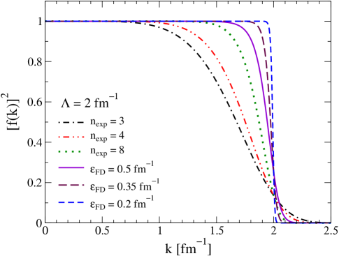
Figure 2: Plots of the exponential and Fermi-Dirac regulators squared as a function of momentum $k$ for $\Lambda=2\,\mbox{fm}^{-1}$ and a range of parameters $n$ and $\epsilon$.

In Fig. 2, the quantity $[f(k)]^{2}$ is plotted against $k$ for fixed cutoff $\Lambda=2\,\mbox{fm}^{-1}$ using some candidate parameterizations of the exponential and Fermi-Dirac forms. While a sharp cutoff (for which $f(k)=\theta(\Lambda-k)$) preserves the on-shell $T$ matrix up to the cutoff, the $T$ matrix for a smooth cutoff is multiplied by $[f(k)]^{2}$, leading to distortions in the phase shifts near the cutoff. The exponential regulator (“exp”) from Eq. (31) with $n=3$ corresponds to what is used in N³LO chiral potentials [16, 17]; it is evident that this regulator applied in the present context will significantly distort the phase shifts for momenta well below $\Lambda$. As $n$ is increased, the regulator gets sharper; for numerical reasons, $n=10$ is probably the practical upper limit. The Fermi-Dirac form (“FD”) interpolates smoothly between sharp and smooth as a function of the $\epsilon$ parameter. It causes less distortion for lower momenta than the exponential regulator.

The effects of different regulators on $V_{{\rm low}\,k}$ potentials with the same starting (“bare”) potential and the same cutoff are illustrated in Fig. 3. In channels where the potential is close to zero at $\Lambda$, such as the ³S₁ partial wave, the differences between sharp and smooth are slight, particularly as the regulator gets sharper ($n_{\rm exp}$ is smoother than $\epsilon_{\rm FD}=0.5\,\mbox{fm}^{-1}$; see Fig. 2). However, the difference in other channels can be striking, as seen in Fig. 3 for the ³D₂ partial wave. The observed cusp-like behavior is due to reproducing the phase shifts for momenta up to the cutoff. The existence of sharp regulator artifacts is not a problem in principle, as the potential is not an observable, but in practice it can lead to convergence problems at the 10–100 keV level in the deuteron and triton.

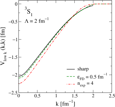
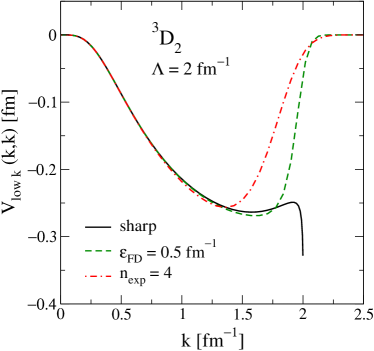
Figure 3: Diagonal matrix elements $V_{{\rm low}\,k}(k,k)$ for $\Lambda=2\,\mbox{fm}^{-1}$, derived from the N³LO chiral potential of Ref. [16] with a sharp and two smooth regulators.

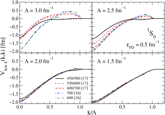
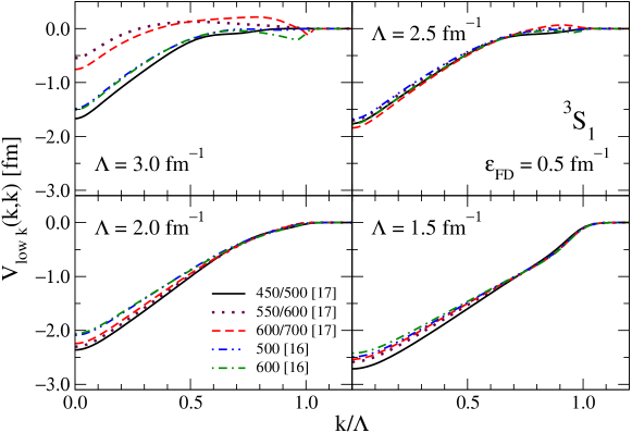
Figure 4: The “collapse” of $V_{{\rm low}\,k}$ interactions derived from N³LO chiral potentials with a Fermi-Dirac regulator ($\epsilon_{\rm FD}=0.5\,\mbox{fm}^{-1}$) as the cutoff is lowered in the ¹S₀ and ³S₁ channels. The diagonal matrix elements $V_{{\rm low}\,k}(k,k)$ are shown, but as in Ref. [2], we find similar results for the off-diagonal matrix elements. The different lines correspond to different starting potentials with the corresponding cutoffs, $\Lambda$ [16] or $\Lambda/\widetilde{\Lambda}$ [17], in MeV given in the legends. For Ref. [17], $\widetilde{\Lambda}$ is the spectral function cutoff.

One of the striking properties of $V_{{\rm low}\,k}$ with a sharp cutoff is the “collapse” of different high-precision NN potentials to almost the same low-momentum potential as the cutoff is lowered below $3\,\mbox{fm}^{-1}$ [2]. This behavior is expected as a consequence of the same long-range pion-exchange interaction together with phase shift equivalence of the potentials up to $k\approx 2.1\,\text{fm}^{-1}$. Therefore, it is not surprising that it remains a property of $V_{{\rm low}\,k}$ interactions derived with smooth regulators, as shown in Fig. 4 for a set of chiral potentials with different initial (“bare”) cutoffs. Note that the low-momentum interactions from different starting potentials are close but not identical. The differences will be paralleled by differences in the corresponding short-range three-body interactions.

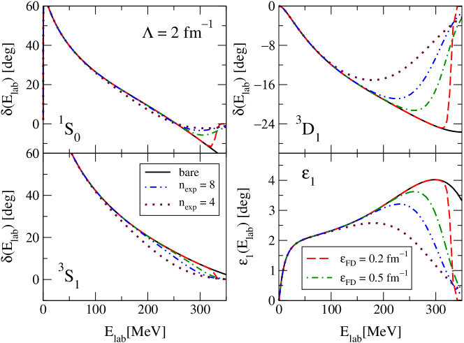
Figure 5: The effects of different regulators on the initial phase shifts $\delta$ and the mixing parameter $\varepsilon_{1}$ as a function of laboratory energy $E_{\rm lab}$ is shown for selected channels. The phase shifts are calculated using the N³LO chiral potential from Ref. [16].

Low-momentum interactions with smooth cutoffs reproduce the initial phase shifts up to factors of the regulator function. The error in phase shifts due to the regulator alone is illustrated in Fig. 5 for some representative two-body phase shifts as a function of laboratory energy. In particular, for each energy, the on-shell T-matrix from a bare potential (in this case the N³LO chiral potential from Ref. [16]) is multiplied by $[f(k)]^{2}$ using the momentum $k$ corresponding to that energy. This corresponds to the distortion that would be present if numerical errors in constructing $V_{{\rm low}\,k}$ were negligible. The latter are documented next and are small. We have no universal rule for deciding whether a distortion is acceptable; it depends on how it propagates to the observable in question. For example, for the low-energy bound-state of the deuteron, none of the distortions in Fig. 5 is important. The distortion is analogous to the error band from a chiral EFT truncation (but we have not formulated a corresponding power counting rule). Therefore, we expect that there is no concern if the distortion is comparable to the EFT truncation error. In addition, for low-energy properties, the error incurred here can be absorbed by the short-range part of the corresponding three-body interactions. Consequently, the propagation of phase-shift errors to many-body observables can only be studied after including three-nucleon forces. It is evident, however, that $n_{\rm exp}=8$ and $\epsilon_{\rm FD}=0.5$ only distort minimally. We will show below that these are also good choices for convergence. In future applications, the regulator effects can be tested by varying the parameters determining the smoothness.

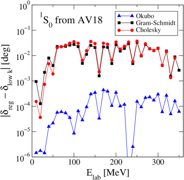
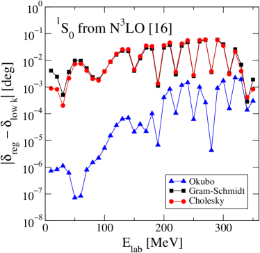
Figure 6: Errors in phase shifts relative to regulated bare phase shifts for three hermitization methods using the exponential regulator with $\Lambda=2\,\mbox{fm}^{-1}$. The potentials used on the left were derived from Argonne $v_{18}$ [13] with $n_{\rm exp}=4$ and those used on the right were derived from the N³LO chiral potential from Ref. [16] with $n_{\rm exp}=8$.

Phase shifts can also differ from those calculated from the input (“bare”) potential because of numerical errors in generating the low-momentum interaction. In Fig. 6, the effects of numerical errors on the phase shifts for different hermitization methods (but fixed regulator) are isolated by plotting the difference of the calculated low-momentum phase shifts and the distorted bare phase shifts. We conclude that the Okubo hermitization is numerically more robust than the Gram-Schmidt or Cholesky methods, with errors in the phase shifts of order $10^{-4}$ degrees below 200 MeV and then varying up to $10^{-3}$ degrees depending on the regulator and the initial potential. Consequently, we use the Okubo hermitization in the following unless otherwise specified. For fixed hermitization but different regulators, we have found that relatively smooth cutoffs (e.g., $\epsilon_{\rm FD}=0.5\,\mbox{fm}^{-1}$) achieve $10^{-4}$ degree accuracy with a moderate (of order 50) Gauss points, but sharper cutoffs (e.g., $\epsilon_{\rm FD}=0.2\,\mbox{fm}^{-1}$) have errors for energies above $E_{\rm lab}=200\,\mbox{MeV}$ that can grow as large as $10^{-1}$ degrees. Greater accuracy can be obtained with a more carefully prescribed distribution of points.

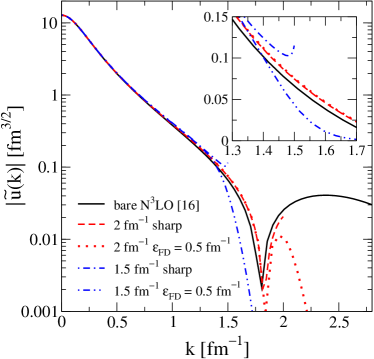
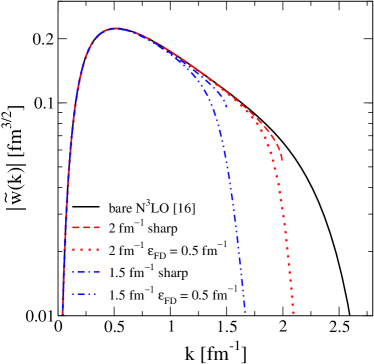
Figure 7: S–state and D–state components of the deuteron wave function in momentum space ($\widetilde{u}(k)$ and $\widetilde{w}(k)$ respectively) for the bare N³LO chiral potential from Ref. [16] and those derived using smooth and sharp cutoffs at $\Lambda=2.0\,\mbox{fm}^{-1}$ and $1.5\,\mbox{fm}^{-1}$.

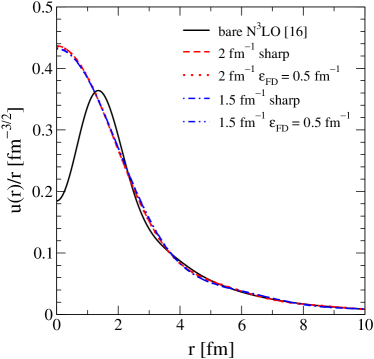
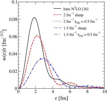
Figure 8: Deuteron wave functions in coordinate space for smooth and sharp cutoffs as in Fig. 7.

The deuteron wave functions for smooth and sharp cutoffs are contrasted in momentum space in Fig. 7 and in coordinate space in Fig. 8. We follow the notation of Ref. [29], with S–wave and D–wave components denoted in coordinate space by $u$ and $w$ respectively, and with tildes in momentum space. They are normalized as $\int_{0}^{\infty}dr\,[u(r)^{2}+w(r)^{2}]=1$ and $\int_{0}^{\infty}dk\,k^{2}\,[\widetilde{u}(k)^{2}+\widetilde{w}(k)^{2}]=1$. The sharp-cutoff wave functions develop cusp-like structure in momentum space below $2\,\mbox{fm}^{-1}$ (see inset in Fig. 7), which are removed by the Fermi-Dirac (or any other smooth) regulator. The different momentum-space behavior is evident in the coordinate-space wave functions as smaller amplitudes in the large-distance oscillations with increasing smoothing (for the S–state component this is visible only under additional magnification). Note that the “wound” in the N³LO coordinate-space wave function is removed by running down the cutoff (we plot $u(r)/r$ to make the suppression near the origin more explicit). This feature of the wave functions leads to more perturbative behavior in nuclear matter [5] as well as in few-body systems [8, 10].

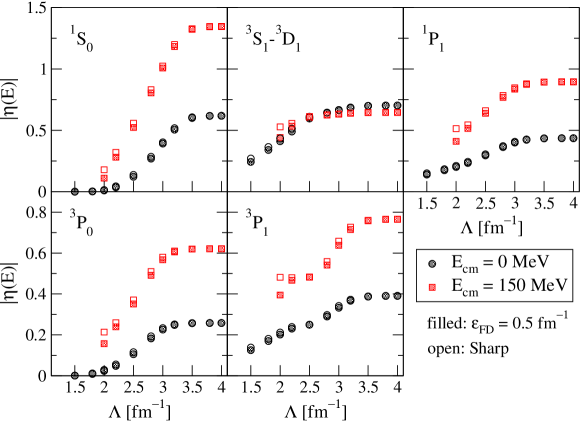
Figure 9: The largest repulsive Weinberg eigenvalues at two energies as a function of cutoff for selected partial waves. The $V_{{\rm low}\,k}$ interactions are derived from the N³LO chiral potential of Ref. [16].

The “perturbativeness” of $V_{{\rm low}\,k}$ interactions with sharp cutoffs was examined in Ref. [8] using Weinberg eigenvalues as a diagnostic. For details on the Weinberg analysis we refer the reader to Refs. [8, 30]. In Fig. 9, we show the largest repulsive Weinberg eigenvalues as a function of the cutoff for selected channels, using the N³LO chiral potential from Ref. [16], which is constructed with a cutoff of 500 MeV. Although this is already a fairly soft potential, we still observe the characteristic decrease with low-momentum cutoff starting as high as $3.5\,\mbox{fm}^{-1}$ (rather than at $2.5\,\mbox{fm}^{-1}$, as one might naively expect). This translates into weaker correlations in many-body wave functions (and therefore better convergence). The rate of decrease is largely independent of the smoothness of the cutoff.

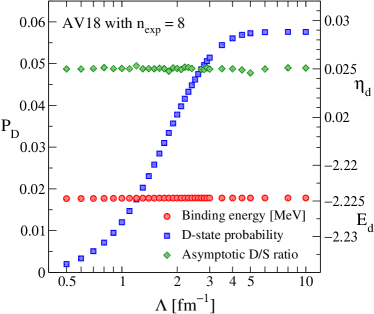
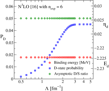
Figure 10: D–state probability $P_{\rm D}$ (left axis), binding energy $E_{d}$ (lower right axis), and asymptotic D/S ratio $\eta_{d}$ (upper right axis) of the deuteron as a function of the cutoff, starting from the Argonne $v_{18}$ [13] (left) and the N³LO chiral potential of Ref. [16] (right) with different smooth regulators.

Various deuteron properties are shown in Fig. 10 as a function of the cutoff using potentials derived from the Argonne $v_{18}$ potential [13] with exponential regulator $n_{\rm exp}=8$ on the left, and from the N³LO chiral potential of Ref. [16] with exponential regulator $n_{\rm exp}=6$ on the right. Plotted on the left axis is the D–state probability $P_{D}$, defined as

$$P_{D}\equiv\int_{0}^{\infty}\!dr\,w(r)^{2}=\int_{0}^{\infty}\!dk\,k^{2}\,\widetilde{w}(k)^{2}\,.$$ (37)

The cutoff dependence reflects the fact that $P_{\rm D}$ is not an observable [31, 32]. The D–state probability evolves with the short-range part of the potential and, in particular, the short-range tensor interaction decreases as the cutoff is lowered. This decrease is desirable to reduce correlations in many-body wave functions [5]. The qualitative change in $P_{\rm D}$ is the same for other regulators and hermitization schemes (the Gram-Schmidt procedure is used in Fig. 10).

In contrast to the D–state probability, the deuteron binding energy $E_{d}$ and the asymptotic D/S ratio $\eta_{d}$ are observables and thus cutoff independent (up to numerical tolerances), as shown by the right axes in Fig. 10. The asymptotic D/S ratio is calculated here by an extrapolation of the ratio of the deuteron wave function D– to S–state components to the deuteron pole at $k^{2}=-mE_{d}$ [31], rather than the conventional approach of extrapolating the ³S₁–³D₁ mixing angle $\varepsilon_{1}$. That is, we evaluate $-\widetilde{w}(k^{2})/\widetilde{u}(k^{2})$ on the Gauss mesh for positive $k^{2}$, and then make a (near-linear) extrapolation to $k^{2}=-mE_{d}$. The constancy of $\eta_{d}$ in Fig. 10 directly refutes the claim of Ref. [33] that this quantity cannot be reproduced using low-momentum interactions.

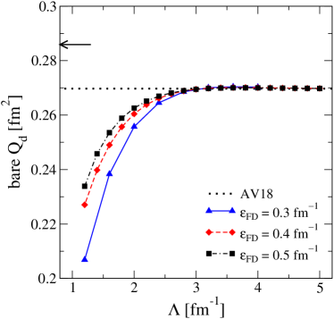
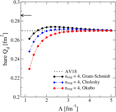
Figure 11: The quadrupole moment of the deuteron $Q_{d}$ calculated with the bare operator as a function of the cutoff for different smoothness regulators (left) and for different hermitization schemes (right). The low-momentum interactions are derived from the Argonne $v_{18}$ potential [13], and the experimental quadrupole moment is indicated with an arrow.

Matrix elements of operators that are dominated by distance scales larger than the inverse cutoff are to a good approximation preserved as the cutoff is lowered. We investigate the evolution of operators by studying the expectation values in the deuteron of the bare quadrupole moment, rms radius and $1/r$ operators. The relevant formulas are [29]

$$Q_{d} =\frac{1}{20}\int_{0}^{\infty}\!dr\,r^{2}\,w(r)\,(\sqrt{8}\,u(r)-w(r))$$

$$=-\frac{1}{20}\int_{0}^{\infty}\!dk\,\biggl{[}\sqrt{8}\,\biggl{(}k^{2}\,\frac{d\widetilde{u}(k)}{dk}\frac{d\widetilde{w}(k)}{dk}+3k\,\widetilde{w}(k)\frac{d\widetilde{u}(k)}{dk}\biggr{)}$$

$$\hskip 170.71652pt+k^{2}\biggl{(}\frac{d\widetilde{w}(k)}{dk}\biggr{)}^{2}+6\,\widetilde{w}(k)^{2}\biggr{]}\,,$$ (38)

$$r_{d} =\frac{1}{2}\biggl{[}\int_{0}^{\infty}\!dr\,r^{2}\,(u(r)^{2}+w(r)^{2})\biggr{]}^{1/2}$$

$$=\frac{1}{2}\biggl{[}\int_{0}^{\infty}\!dk\,\biggl{\{}\biggl{(}k\,\frac{d\widetilde{u}(k)}{dk}\biggr{)}^{2}+\biggl{(}k\,\frac{d\widetilde{w}(k)}{dk}\biggr{)}^{2}+6\,\widetilde{w}(k)^{2}\biggr{\}}\biggr{]}^{1/2}\,,$$ (39)

and

$$\langle 1/r\rangle=\int_{0}^{\infty}\!dr\,\frac{1}{r}\,[u(r)^{2}+w(r)^{2}]\,.$$ (40)

(We note that the momentum-space expressions for $Q_{d}$ and $r_{d}$ show that these are only well-defined for a smooth cutoff [29].) These operators are dominated by the long-range part of the interaction, and therefore we expect that the expectation values change only for low cutoffs. This is verified in Fig. 11, where we show the deuteron quadrupole moment $Q_{d}$ as a function of the cutoff for different smoothness regulators (left) and for different hermitization schemes (right), and in Figs. 12 and 13, where the rms radius $r_{d}$ and the matrix element of $1/r$ are plotted as a function of $\Lambda$.

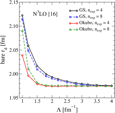
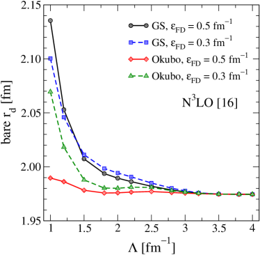
Figure 12: The rms radius $r_{d}$ of the deuteron calculated with the bare operator as a function of the cutoff for different regulators and hermitization schemes. The low-momentum interactions are derived using the N³LO chiral potential from Ref. [16].

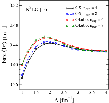
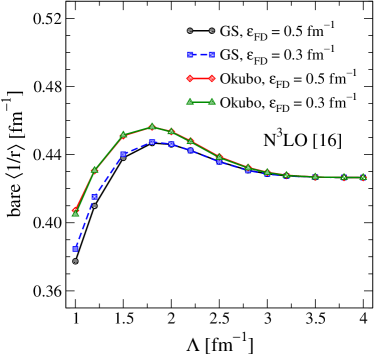
Figure 13: The matrix element of $1/r$ in the deuteron calculated with the bare operator as a function of the cutoff for different regulators and hermitization schemes. The low-momentum interactions are derived using the N³LO chiral potential from Ref. [16].

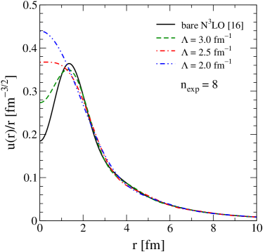
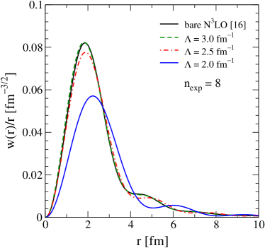
Figure 14: Deuteron wave functions in coordinate space for low-momentum interactions at several different cutoffs using an exponential regulator with $n_{\rm exp}=8$. The initial interaction is the N³LO chiral potential from Ref. [16].

We emphasize that the bare quadrupole moment by itself does not correspond to an experimental observable. To correctly reproduce the experimental moment (indicated in Fig. 11 by an arrow), one needs the corresponding operators. We find that the change of the quadrupole moment is of the same magnitude as the difference between the bare and experimental quadrupole moments for cutoffs down to $1.5$–$2\,\mbox{fm}^{-1}$. From the deuteron wave functions shown in Fig. 14, we conclude that low-energy observables in the deuteron are reproduced without short-range correlations in the wave function. Similar observations hold for the expectation values of the rms radius $r_{d}$ and of the $1/r$ operator.

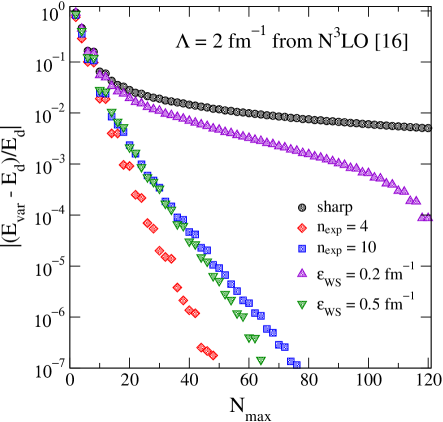
Figure 15: The relative error in the deuteron binding energy $E_{d}$ as a function of the size of the oscillator space for sharp cutoff and various smooth regulators.

The key motivation for smooth cutoffs was to remedy the slow convergence at the 10 keV level in the deuteron and at the 100 keV level in the triton, when calculated in a harmonic oscillator basis. In Fig. 15, the relative error in the binding energy of the deuteron (with respect to the converged result) is shown as a function of the size of the oscillator space ($N_{\rm max}\,\hbar\omega$ excitations) for a range of regulators. The slow convergence is evident for the sharp cutoff, where the error is below the percent level only for the largest space. The Fermi-Dirac regulator with $\epsilon=0.2\,\text{fm}^{-1}$, which is still very sharp (see Fig. 2), gives improved errors but still requires large spaces. Increasing $\epsilon$ from $0.2\,\text{fm}^{-1}$ to $0.5\,\text{fm}^{-1}$ steadily decreases the error until it improves rapidly with the space size, while still only minimally distorting phase shifts. Very similar relative errors are obtained for the exponential regulator with $n=8$ (not shown) or $n=10$. Lowering $n$ to $4$ reduces the error still further, but at the cost of a potentially significant distortion of the phase shifts.

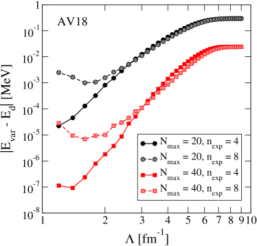
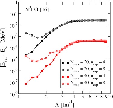
Figure 16: The absolute error in the deuteron binding energy $E_{d}$ calculated from low-momentum interactions derived using the Argonne $v_{18}$ potential [13] (left) and the N³LO chiral potential from Ref. [16] (right) as a function of the cutoff. We show results for two oscillator spaces and for two different exponential regulators.

The absolute error in the deuteron binding energy is shown in Fig. 16 as a function of the cutoff for low-momentum interactions derived from the Argonne $v_{18}$ [13] and the N³LO chiral potential from Ref. [16]. In all cases, the reproduction of the binding energy improves with decreasing cutoff until the limits of numerical accuracy are reached. This is in contrast to the observed degradation below $2\,\mbox{fm}^{-1}$ for a sharp cutoff [9]. The improvement for the N³LO potential starts just below $4\,\mbox{fm}^{-1}$ (even though the EFT cutoff is 500 MeV or $2.5\,\mbox{fm}^{-1}$) and is quite significant by $2\,\mbox{fm}^{-1}$.

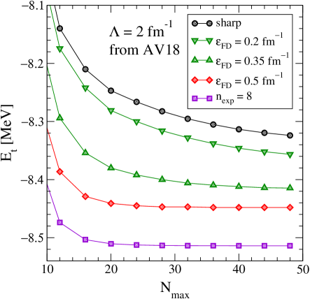
Figure 17: The triton binding energy $E_{t}$ as a function of the size of the oscillator space, for different smoothness regulators starting from the the Argonne $v_{18}$ potential [13].

The convergence is also greatly improved for the triton. In Fig. 17, the triton binding energy is plotted as a function of the size of the oscillator space. For efficiency, convergence for the smallest possible space is desirable, as the computational cost grows rapidly with $N_{\rm max}$ and for larger systems. Convergence at the keV level is achieved by all exponential regulators with $n\geqslant 4$ ($n_{\rm exp}=8$ is shown) soon after $N_{\rm max}=20$. The consequence in moving from sharp to increasingly smooth regulators is seen from the Fermi-Dirac regulators, where $\epsilon=0.5\,\text{fm}^{-1}$ yields very satisfactory results. The difference between converged results for the triton is a measure of the differences in the short-range three-body force with the different regulators.

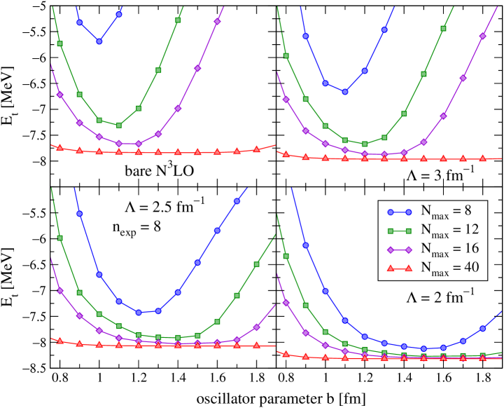
Figure 18: Dependence of the triton binding energy $E_{t}$ as a function of oscillator parameter $b$ for the bare N³LO chiral potential of Ref. [16] (upper left) and evolved to low momenta $\Lambda=3.0,2.5$ and $2.0\,\mbox{fm}^{-1}$ with exponential regulator $n_{\rm exp}=8$. Results are presented for three smaller spaces $N_{\rm max}=8,12$ and $16$, along with the converged $N_{\rm max}=40$ energy.

The dramatically improved convergence of lower cutoffs compared to even the soft N³LO chiral potential is demonstrated in Fig. 18. Note that the phase shifts would be essentially undistorted at $\Lambda=2.5\,\mbox{fm}^{-1}$. In addition, when we evolve the potential to low cutoffs, the dependence on the oscillator parameter $b$ becomes flatter for a given $N_{\rm max}$, and for $\Lambda=2.0\,\mbox{fm}^{-1}$ the minimum is unchanged as the space is enlarged. The sharp-cutoff $V_{{\rm low}\,k}$ also shows a flatter dependence on the oscillator parameter compared to the initial N³LO chiral potential and converges rapidly to the 100 keV level, but then converges slowly (the convergence for the N³LO chiral potential is very similar to that shown for the Argonne $v_{18}$ potential in Fig. 17).

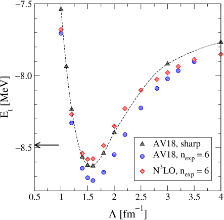
Figure 19: The triton binding energy $E_{t}$ as a function of the cutoff starting from the Argonne $v_{18}$ potential [13] with a sharp cutoff (taken from the Faddeev calculations of Ref. [4]) and with an exponential regulator. We also show results for the N³LO chiral potential of Ref. [16] with the same exponential regulator.

In Fig. 19, the triton binding energy as a function of the cutoff is shown with the exponential regulator $n_{\rm exp}=6$ calculated from the Argonne $v_{18}$ [13] and using the N³LO chiral potential of Ref. [16]. For comparison, we also show the Faddeev results from Ref. [4], which use a sharp cutoff. The triton binding energy is cutoff dependent because we have not included the corresponding three-body interactions. Therefore, the difference to the experimental binding energy (shown with an arrow) is the total three-body contribution. The pattern of running is very similar in the three cases, although the values for a given regulator naturally vary. While it is possible to choose a cutoff so that the experimental triton binding energy is reproduced by only the two-body interaction, the total three-body contribution will not vanish in other systems (e.g., the alpha particle [4] or nuclear matter [5]).

5 Summary and Conclusions

In this paper, low-momentum “$V_{{\rm low}\,k}$” interactions with smooth cutoffs were constructed and tested for several different types of regulators and hermitization schemes. Problems seen in previous work with variational calculations that were attributed to artifacts from a sharp cutoff are resolved by smooth regulators. In particular, convergence for the energy of the deuteron and triton in a harmonic oscillator basis is greatly improved. We have checked that this conclusion also holds for other variational trial wave functions not shown here. We expect this improved convergence to carry over to other few- and many-body systems.

The regulators introduced here are specified not only by the cutoff on relative momenta but by a parameter that determines the smoothness. Our conclusions for the optimal regulator are provisional, because this work has been restricted to convergence rates in the deuteron and the triton. However, based on the observed convergence it appears that a similar degree of smoothness is optimal for different regulators. This is achieved with $n\approx 8$ for the exponential regulator or $\epsilon\approx 0.5\,\text{fm}^{-1}$ for the Fermi-Dirac regulator. Going to smoother regulators maintains the same rapid convergence but will increase distortions of the phase shifts. Whether or not this is an issue depends on the application, but we expect that the latter is not a problem for low-energy observables.

Given the regulator freedom that exists in generating low-momentum interactions for a given cutoff $\Lambda$, it is clearly a misnomer to speak of “the” $V_{{\rm low}\,k}$ potential. We emphasize in particular that the consistent three-body (and higher many-body) interactions corresponding to the smooth two-body interaction will differ in each case. More precisely, since the long-distance (pion-exchange) parts of the interaction are preserved by the RG (until the cutoff is comparable to the pion mass), the short-distance part of the three-body interaction is modified. Cutoff and regulator independence with two-body interactions alone should not be a criterion for the applicability of low-momentum interactions to nuclear structure. (Note that this perspective differs markedly from that expressed in Ref. [34], which discussed the application of low-momentum potentials with sharp cutoffs to few-nucleon systems.) Rather, the three-body variations for different regulators allow us to extend the powerful test of cutoff independence for observables to include independence of the regulator. However, without a consistent three-body interaction, few- and many-body calculations are largely meaningless (except for considerations of convergence). Therefore, a high priority for the near term is to develop the machinery to quickly fit approximate three-body interactions for a given regulator.

The methods described here apply equally to low-momentum interactions derived from conventional nucleon-nucleon potentials and to those derived from chiral EFT potentials. The latter has the advantage of a systematic organization of many-body forces and operators. While chiral EFT potentials already start from lower cutoffs than conventional NN interactions, we find significant added advantages for few- and many-body calculations by starting with chiral potentials fit at a larger cutoff and running them down to a lower cutoff [5, 8].

Field redefinitions in EFT reshuffle higher-order terms so that the truncation error is different but of the same order. That is, if the EFT is specified to NLO, then N²LO terms will differ after a field redefinition but the expected truncation error is still N²LO. The RG transformations discussed here preserve the error as the cutoff is lowered by generating all necessary higher-order short-range operators through the evolution. This is particularly advantageous when the running is rapid and the separation of scales is not large, as in the nuclear case (when the tensor force is active). At present, only the two-body interaction is evolved while the three-body interaction is fit for each cutoff using the N²LO form [4]. While there are solid indications that this is a reasonable procedure [4], the evolution of consistent chiral three-body interactions to lower momenta is a major goal. In addition, the smooth regulators discussed here may have advantages for constructing chiral EFT potentials with low cutoffs. As is apparent from Fig. 2, the exponential regulator with $n\approx 8$ and the Fermi-Dirac regulator with $\epsilon\approx 0.5\,\text{fm}^{-1}$ lead to weaker distortions than the conventional exponential regulator with $n=3$ in the N³LO chiral potentials [16, 17], and thus smaller errors have to be absorbed by the counterterms.

There are immediate applications that can be made using the low-momentum interactions with smooth cutoffs developed here. Variational calculations using hyperspherical harmonics [35], the No-Core Shell Model [36] and the Coupled-Cluster approach [37] should benefit from the improved convergence. Tests for all of these are in progress.

References

- [1] S.K. Bogner, T.T.S. Kuo, A. Schwenk, D.R. Entem and R. Machleidt, Phys. Lett. B 576 (2003) 265.
- [2] S.K. Bogner, T.T.S. Kuo and A. Schwenk, Phys. Rept. 386 (2003) 1.
- [3] S.K. Bogner, A. Schwenk, T.T.S. Kuo and G.E. Brown, nucl-th/0111042.
- [4] A. Nogga, S.K. Bogner and A. Schwenk, Phys. Rev. C70 (2004) 061002(R).
- [5] S.K. Bogner, A. Schwenk, R.J. Furnstahl and A. Nogga, Nucl. Phys. A763 (2005) 59.
- [6] S.K. Bogner, T.T.S. Kuo, L. Coraggio, A. Covello and N. Itaco, Phys. Rev. C65 (2002) 051301(R).
- [7] A. Schwenk and A.P. Zuker, nucl-th/0501038.
- [8] S.K. Bogner, R.J. Furnstahl, S. Ramanan and A. Schwenk, Nucl. Phys. A773 (2006) 203.
- [9] S.K. Bogner and R.J. Furnstahl, Phys. Lett. B632 (2006) 501.
- [10] S.K. Bogner and R.J. Furnstahl, Phys. Lett. B639 (2006) 237.
- [11] D.J. Dean, G. Hagen, T. Papenbrock, A. Schwenk and A. Nogga, in preparation.
- [12] E. Epelbaoum, W. Glöckle, A. Krüger and U.G. Meißner, Nucl. Phys. A645 (1999) 413.
- [13] R.B. Wiringa, V.G.J. Stoks and R. Schiavilla, Phys. Rev. C51 (1995) 38.
- [14] S.-B. Liao, J. Polonyi and M. Strickland, Nucl. Phys. B567 (2000) 493, and references therein.
- [15] G.P. Lepage, “How to Renormalize the Schrödinger Equation”, Lectures given at 9th Jorge Andre Swieca Summer School: Particles and Fields, Sao Paulo, Brazil, February, 1997, nucl-th/9706029.
- [16] D.R. Entem and R. Machleidt, Phys. Rev. C68 (2003) 041001(R).
- [17] E. Epelbaum, W. Glöckle and U.G. Meißner, Nucl. Phys. A747 (2005) 362.
- [18] M.C. Birse, J.A. McGovern and K.G. Richardson, Phys. Lett. B464 (1999) 169.
- [19] W.H. Press, S.A. Teukolsky, W.T. Vetterling and B.P. Flannery, Numerical Recipes in C, Cambridge University Press, 1992.
- [20] J.D. Holt, T.T.S. Kuo, G.E. Brown, Phys. Rev. C69 (2004) 034329.
- [21] S.Y. Lee and K. Suzuki, Phys. Lett. B91 (1980) 173.
- [22] K. Suzuki and S.Y. Lee, Prog. Theor. Phys. 64 (1980) 2091.
- [23] S. Okubo, Prog. Theor. Phys. 12 (1954) 603.
- [24] K. Suzuki and R. Okamoto, Prog. Theor. Phys. 70 (183) 439.
- [25] F. Andreozzi, Phys. Rev. C54 (2004) 684.
- [26] L. Giraud, J. Langou and M. Rozloznik, Computer and Mathematics with Applications 50 (2005) 1069.
- [27] K. Hebeler, private communication.
- [28] J.I. Latorre and T.R. Morris, Int. J. Mod. Phys. A16 (2001) 2071.
- [29] E. Epelbaum, W. Glöckle and U.G. Meißner, Nucl. Phys. A671 (2000) 295.
- [30] S. Weinberg, Phys. Rev. 131 (1963) 440.
- [31] R.D. Amado, Phys. Rev. C19 (1979) 1473.
- [32] J.L. Friar, Phys. Rev. C20 (1979) 325.
- [33] S.X. Nakamura, Prog. Theor. Phys. 114 (2005) 77.
- [34] S. Fujii, E. Epelbaum, H. Kamada, R. Okamoto, K. Suzuki and W. Glöckle, Phys. Rev. C70 (2004) 024003.
- [35] M. Viviani, L.E. Marcucci, S. Rosati, A. Kievsky and L. Girlanda, nucl-th/0512077.
- [36] P. Navratil, J.P. Vary and B.R. Barrett, Phys. Rev. C62 (2000) 054311.
- [37] M. Wloch, D.J. Dean, J.R. Gour, M. Hjorth-Jensen, K. Kowalski, T. Papenbrock and P. Piecuch, Phys. Rev. Lett. 94 (2005) 212501.