Two-level interacting boson models beyond the mean field

Abstract

The phase diagram of two-level boson Hamiltonians, including the Interacting Boson Model (IBM), is studied beyond the standard mean field approximation using the Holstein-Primakoff mapping. The limitations of the usual intrinsic state (mean field) formalism concerning finite-size effects are pointed out. The analytic results are compared to numerics obtained from exact diagonalizations. Excitation energies and occupation numbers are studied in different model space regions (Casten triangle for IBM) and especially at the critical points.

I Introduction

The concepts of phase transition and critical points are defined, strictly speaking for macroscopic systems. However, it has been recently suggested that precursors of phase transitions can be observed in finite-size mesoscopic systems Iachello and Zamfir (2004). In Nuclear Physics the different nuclear shapes and the phase transitions between them are conveniently studied within the Interacting Boson Model (IBM) Iachello and Arima (1987). This was early recognized after the introduction of the model Dieperink et al. (1980); Feng et al. (81); Dukelsky et al. (1984); Frank (1989); López-Moreno and Castaños (1996) but has been studied thoroughly in the last few years Cejnar and Jolie (2000); Jolie et al. (2002); Cejnar et al. (2003); Arias et al. (2003a, b); Rowe (2004); Turner and Rowe (2005); Rosensteel and Rowe (2005); Rowe and Thiamova (2005); Cejnar et al. (2005); Heinze et al. (2006) after the introduction of the concept of critical point symmetries Iachello (2000, 2001, 2003). Since the IBM is formulated from the beginning in terms of creation and annihilation boson operators, its geometric interpretation in terms of shape variables is usually done by introducing a boson condensate with two shape parameters, $\beta$ and $\gamma$ (order parameters) Ginocchio and Kirson (1980); Dieperink et al. (1980). The parameter $\beta$ is related to the axial deformation of the system, while $\gamma$ measures the deviation from axial symmetry. The equilibrium shape of the system is obtained by minimizing the expectation value of the Hamiltonian in the intrinsic state. Shape phase transitions are studied theoretically using one (or a few) control parameter(s) in the Hamiltonian. These control parameters drive the system in different phases characterized by order parameters and allows one to study in a simple way phase transitions and critical points in Nuclear Physics.

The phase diagram of the IBM has been studied with several approaches Cejnar and Jolie (2000); Jolie et al. (2002); Cejnar et al. (2003); Arias et al. (2003a, b); Turner and Rowe (2005); Rowe and Thiamova (2005); Cejnar et al. (2005); Heinze et al. (2006) and it is well known that the dynamical symmetry associated to $U(5)$ corresponds to a spherical shape ($\beta=0$), the dynamical symmetry $SU(3)$ is associated to an axially deformed shape ($\gamma=0,\pi/3,~{}\beta\neq 0$) and the dynamical symmetry $O(6)$ is related to a $\gamma$-unstable deformed shape ($\beta\neq 0$ and $\gamma$-independent). These symmetry limits are usually represented as the vertices of a triangle (Casten triangle) Casten (1990). Phase transitions between these shapes have been widely studied and it is known that the phase transition from $U(5)$ to $O(6)$ is second order while any other transition within the Casten triangle from a spherical to a deformed shape is first order Jolie et al. (2002); Arias et al. (2003b). These studies have been performed, as mentioned above, by using the intrinsic state formalism. However, it is known that this approximate method is only correct at leading order in a $1/N$ expansion where $N$ is the number of bosons. In this paper, we present a method to go beyond this order and compute finite-size corrections to several spectroscopic observables. We stress that $1/N$ corrections obtained with the intrinsic state formalism (or Hartree-Bose method) are in general incorrect and give no information on the proper finite-size corrections.

The paper is organized as follows: first the model Hamiltonian is introduced in Sect. II. In Sect. III, the Holstein-Primakoff mapping Holstein and Primakoff (1940) is performed leading to a boson Hamiltonian in which we retain terms in orders $N$, $N^{1/2}$ and $N^{0}$. Then a Bogoliubov transformation is performed to diagonalize the Hamiltonian and to study both the symmetric (spherical) and the broken (deformed) phases. All this is done in general for two-level boson models in which the lowest level is a scalar ($s$) boson while the upper level is an arbitrary $L$ boson. The IBM corresponds to the particular case $L=2$ ($d_{\mu}$ bosons). In addition to the IBM, we present results for the case $L=0$ as an illustration of the general method. In Sect. IV we compare the analytical results with exact numerical diagonalizations for different paths along the Casten triangle. Finally, Sect. V is for the summary and conclusions.

II The Model

As it has been noted before Turner and Rowe (2005), the experimental exploration of the shape transition and critical points in nuclei is difficult due to the lack of a continuous control parameter. However, in theoretical studies this limitation is overcome by using a Hamiltonian written in terms of one or more control parameters that can vary continuously. In this work, we consider a two-level boson model in which the lowest level is characterized by a zero angular momentum ($s$-boson) while the upper level has an arbitrary angular momentum $L$. The Hamiltonian proposed is a generalization of the IBM consistent-Q formalism (CQF) Warner and Casten (1982), which depends on two control parameters $x$ and $\chi$

$$H=x\>n_{L}-\frac{1-x}{N}Q^{\chi}\cdot Q^{\chi},$$ (1)

where $n_{L}=\sum_{\mu}L^{\dagger}_{\mu}L_{\mu}$ is the operator for the number of bosons in the upper level, $N$ is the total number of bosons, the symbol $\cdot$ stands for the scalar product defined as $a\cdot b=\sum_{\mu=-L}^{+L}(-1)^{\mu}a_{\mu}b_{-\mu}$, and $Q^{\chi}$ is a multipole operator written as,

$$Q_{\mu}^{\chi}=(s^{\dagger}{\tilde{L}^{\phantom{\dagger}}}+L^{\dagger}{s^{\phantom{\dagger}}})^{(L)}_{\mu}+\chi[L^{\dagger}\times{\tilde{L}^{\phantom{\dagger}}}]^{(L)}_{\mu},$$ (2)

where ${\tilde{L}^{\phantom{\dagger}}}_{\mu}=(-1)^{\mu}{L^{\phantom{\dagger}}}_{-\mu}$. For $L=2$, ($d$-bosons) the Hamiltonian (1) is the well-known CQF Hamiltonian for IBM. Though it is not the most general IBM Hamiltonian, it captures the most important low energy properties of a wide range of nuclei Warner and Casten (1983); Chou et al. (1997); Fossion et al. (2002). In particular, it is general enough to describe different nuclear phases and quantum phase transitions, and it has been used for that purpose at the mean field level Jolie et al. (2002); Arias et al. (2003b); Cejnar et al. (2003).

The Hamiltonian (1) comprises different models depending on the value of $L$. For instance, for $L=1$ the Hamiltonian is appropriate for studying the phase diagram of the vibron model Iachello and Levine (1995) of interest in Molecular Physics.

III Mean field and beyond

The usual way of getting the phase diagram of the model (1) is to introduce shape variables. This can be done by considering the intrinsic state formalism, also called Hartree-Bose approximation, Ginocchio and Kirson (1980); Dieperink et al. (1980); Dieperink and Scholten (1980); Dukelsky et al. (1984). In this approach, the ground state is a variational state built out of a condensate of “dressed” bosons, that are independent bosons moving in the average nuclear field. For $L=2$, these bosons are defined as

$$\Gamma^{\dagger}_{c}=\frac{1}{\sqrt{1+\beta^{2}}}\left(s^{\dagger}+\beta\cos\gamma\,d^{\dagger}_{0}+\frac{1}{\sqrt{2}}\beta\sin\gamma\,(d^{\dagger}_{2}+d^{\dagger}_{-2})\right),$$ (3)

and the $N$ boson condensate is,

$$|c\rangle=\frac{1}{\sqrt{N!}}(\Gamma^{\dagger}_{c})^{N}|0\rangle.$$ (4)

The variational variables $\beta$ and $\gamma$ are the order parameters of the system and their equilibrium values are fixed by minimizing the expectation value of the energy. The expression of this energy can be found in many references Ginocchio and Kirson (1980); Dieperink et al. (1980); Dieperink and Scholten (1980); García-Ramos et al. (1998) and can be written schematically as follows,

$$E(N,~{}\beta,~{}\gamma,~{}x,~{}\chi)=NF^{(1)}(N,~{}\beta,~{}\gamma,~{}x,~{}\chi)+(N-1)F^{(2)}(N,~{}\beta,~{}\gamma,~{}x,~{}\chi),$$ (5)

where $F^{(1)}(N,~{}\beta,~{}\gamma,~{}x,~{}\chi)$ is the matrix element of the one-body operators divided by $N$ and $F^{(2)}(N,~{}\beta,~{}\gamma,~{}x,~{}\chi)$ is the matrix element of the two-body operators divided by $N-1$. Note that there is no $N^{2}$ dependence in the two-body operator due to the definition of the Hamiltonian. Actually, the only relevant contribution is the leading one (order $N$) since the next one ($N^{0}$ for instance) are incomplete as explained below.

For the standard IBM Hamiltonian ($L=2$), with an attractive quadrupole interaction, the nucleus always becomes axially deformed, either prolate ($\gamma=0$) for $\chi<0$ or oblate ($\gamma=\pi/3$) for $\chi>0$. As a consequence, the parameter $\gamma$ can be incorporated in the value of $\beta$. $\beta>0$ corresponds to $\gamma=0$ while negative $\beta$ implies $\gamma=\pi/3$. In the case $\chi=0$ the nucleus becomes $\gamma$ unstable, i. e., the energy is independent of $\gamma$.

In this framework, one-phonon excitations above the ground state are constructed by directly replacing in the ground state (4) a condesate boson by an excited boson (TDA method) or by including ground state fluctuations (RPA method) Dukelsky et al. (1984); Leviatan (1987); García-Ramos et al. (1998). For $L=2$, there are five excited phonons that are characterized by their angular momentum projection $K$ and can be labelled as: $\beta$-excitation with $K=0$, $\gamma$-excitations with $K=\pm 2$ and finally two $K=\pm 1$ excitations. It should be noted that not all the excited phonons are always physical, some of them become spurious, Goldstone bosons associated with broken symmetries. This is the case for axially deformed nuclei, the $K=\pm 1$ excitations are Goldstone, spurious bosons because the state constructed with this excitation corresponds to a $O(3)$ rotation of the whole system. In the case of $\gamma$ unstable nuclei, the $K=\pm 2$ excitations also become Goldstone bosons and are related with $O(5)$ rotations of the ground state. In the case of $L=0$ only a $K=0$ excitation exists and it is directly related, as we will see, with the $\beta$ band of the IBM Vidal et al. (2006).

The mean field description of the ground state energy just mentioned is only valid at order $N$. The first quantum corrections can be obtained within the RPA formalism. Alternatively, the Holstein-Primakoff expansion Holstein and Primakoff (1940) offers a simple and natural expansion in powers of $1/N$. The advantages of this transformation are: it is Hermitian, preserves the boson commutation relation, provides a correct expansion in powers of $N$ and its leading order coincides with the mean field contribution.

The Holstein-Primakoff expansion consist in eliminating the $s$-boson transforming the bilinear boson operators in the following way,

$$L^{\dagger}_{\mu}L_{\nu} = b^{\dagger}_{\mu}{b^{\phantom{\dagger}}}_{\nu},$$ (6)

$$L^{\dagger}_{\mu}{s^{\phantom{\dagger}}} = N^{1/2}b^{\dagger}_{\mu}(1-n_{b}/N)^{1/2}=(s^{\dagger}L_{\mu})^{\dagger},$$ (7)

$$s^{\dagger}{s^{\phantom{\dagger}}} = N-n_{b},$$ (8)

where the $b$-bosons satisfy $[{b^{\phantom{\dagger}}}_{\mu},b^{\dagger}_{\nu}]=\delta_{\mu,\nu}$. The mapping fulfils the commutation relations at each order in $N$ in the Taylor expansion of the square root.

We next introduce the $c$-bosons through a shift transformation

$$b^{\dagger}_{\mu}=\sqrt{N}\lambda^{*}_{\mu}+c^{\dagger}_{\mu},$$ (9)

where the $\lambda_{\mu}$’s are complex numbers which form a $(2L+1)$-dimensional vector. This shift allows for a macroscopic occupation number $n_{b}$. Thus, it allows to consider at the same time the spherical, setting $\lambda_{\mu}=0$ for all $\mu$, and the deformed phase, $\lambda_{\mu}\neq 0$. In this latter situation, we shall only consider the case $\lambda_{0}\neq 0$ without loss of generality. The Hamiltonian then reads,

$$H = N^{1}\lambda_{0}^{2}\left\{5x-4-4(x-1)\lambda_{0}^{2}+(x-1)\chi\alpha^{(L)}_{0,0}\lambda_{0}\left[4(1-\lambda_{0}^{2})^{1/2}+\chi\alpha^{(L)}_{0,0}\lambda_{0}\right]\right\}+$$ (10)

$$N^{1/2}\lambda_{0}\left(c^{\dagger}_{0}+{c^{\phantom{\dagger}}}_{0}\right)\left\{5x-4-8\lambda_{0}^{2}(x-1)+2(x-1)\chi\alpha^{(L)}_{0,0}\lambda_{0}\left[{-4\lambda_{0}^{2}+3\over(1-\lambda_{0}^{2})^{1/2}}+\chi\alpha^{(L)}_{0,0}\lambda_{0}\right]\right\}+$$

$$N^{0}\Bigg{\{}\left[3x-2-6\lambda_{0}^{2}(x-1)\right]n_{c}+(x-1)\left[(2L+1)-(2L+3)\lambda_{0}^{2}+\left(1-\lambda_{0}^{2}\right)\left(P^{\dagger}_{c}+{P^{\phantom{\dagger}}}_{c}\right)-4\lambda_{0}^{2}\left({c^{\dagger}_{0}}^{2}+2c^{\dagger}_{0}{c^{\phantom{\dagger}}}_{0}+{c^{\phantom{\dagger}}}_{0}^{2}\right)\right]+$$

$$2\chi(x-1)\Bigg{\{}\lambda_{0}(1-\lambda_{0}^{2})^{1/2}\Bigg{[}\sum_{\mu=-L}^{+L}\alpha^{(L)}_{0,\mu}+2c^{\dagger}_{\mu}{c^{\phantom{\dagger}}}_{\mu}\left[(-1)^{\mu}\alpha^{(L)}_{\mu,-\mu}+\alpha^{(L)}_{0,\mu}\right]+(-1)^{\mu}\alpha^{(L)}_{\mu,0}\left(c^{\dagger}_{\mu}c^{\dagger}_{-\mu}+{c^{\phantom{\dagger}}}_{\mu}{c^{\phantom{\dagger}}}_{-\mu}\right)\Bigg{]}$$

$$-{\lambda_{0}^{3}\alpha^{(L)}_{0,0}\over 2(1-\lambda_{0}^{2})^{1/2}}\Bigg{[}2+3\left({c^{\dagger}_{0}}^{2}+2c^{\dagger}_{0}{c^{\phantom{\dagger}}}_{0}+{c^{\phantom{\dagger}}}_{0}^{2}\right)+2n_{c}\Bigg{]}-{\lambda_{0}^{5}\alpha^{(L)}_{0,0}\over 4(1-\lambda_{0}^{2})^{3/2}}\left(1+{c^{\dagger}_{0}}^{2}+2c^{\dagger}_{0}{c^{\phantom{\dagger}}}_{0}+{c^{\phantom{\dagger}}}_{0}^{2}\right)\Bigg{\}}+$$

$$+\chi^{2}(x-1)\lambda_{0}^{2}\Bigg{\{}1+\sum_{\mu=-L}^{+L}2c^{\dagger}_{\mu}{c^{\phantom{\dagger}}}_{\mu}\left[(-1)^{\mu}\alpha^{(L)}_{0,0}\alpha^{(L)}_{\mu,-\mu}+{\alpha^{(L)}_{0,\mu}}^{2}\right]+(-1)^{\mu}{\alpha^{(L)}_{0,\mu}}^{2}\left(c^{\dagger}_{\mu}c^{\dagger}_{-\mu}+{c^{\phantom{\dagger}}}_{\mu}{c^{\phantom{\dagger}}}_{-\mu}\right)\Bigg{\}}\Bigg{\}}+O(1/\sqrt{N}),$$

$$= H_{1}+H_{1/2}+H_{0}+O(1/\sqrt{N}),$$ (11)

where $\alpha^{(L)}_{\mu,\nu}=\langle L,\mu;L\nu|L,\mu+\nu\rangle$ and $P^{\dagger}_{c}=c^{\dagger}\cdot c^{\dagger}=({P^{\phantom{\dagger}}}_{c})^{\dagger}$.

The term of order $N$ $(H_{1})$ is exactly the mean-field energy. Setting $\lambda=\beta/{\sqrt{1+\beta^{2}}}$ one gets,

$$E(N,~{}\beta,~{}x,~{}y)=N{\beta^{2}\over(1+\beta^{2})^{2}}\Big{[}5x-4+x\beta^{2}+\beta y(x-1)(4+\beta y)\Big{]},$$ (12)

where $y=\chi\alpha^{(L)}_{0,0}$. In the case of $L=2$, equation (12) reduces to the IBM ground state energy. Note that $H_{1}$ only depends on $L$ through the Clebsch-Gordan coefficient $\langle L,\mu;L\nu|L,\mu+\nu\rangle$ although this dependence can be absorbed in the parameter $y$.

Figure 1: Qualitative phase diagram for the Hamiltonian (1) and $L=2$. The insets show typical energy surfaces versus the deformation parameter $\beta$ in each of the phases and at the phase borders. The control variables of the diagram are defined as $\rho=1-x$ and $\phi=\frac{2\pi}{3\sqrt{7}}~{}(\frac{\sqrt{7}}{2}+\chi)$.

$H_{1}$ provides the mean field energy and therefore the equilibrium values of the order parameter. In Fig. 1 is depicted the phase diagram corresponding to $H_{1}$. For given parameters $x$ and $\chi(y)$, the first step consists in minimizing $H_{1}$ with respect to $\beta(\lambda)$ getting the equilibrium value $\beta_{0}(\lambda_{0})$. The study of these minima have been shown in several publications Feng et al. (81); López-Moreno and Castaños (1996), but for completeness we summarize here the main features:

• $\beta=0$ is always a stationary point. For $x<4/5$, $\beta=0$ is a maximum while for $x>4/5$ becomes a minimum. In the case of $x=4/5$, $\beta=0$ is an inflection point. $x=4/5$ is the point in which a minimum at $\beta=0$ starts to develop and defines the antispinodal line.

• For $\chi\neq 0~{}(y\neq 0)$ there exists a region, where two minima, one spherical and one deformed, coexist. This region is defined by the point where the $\beta=0$ minimum appears (antispinodal point) and the point where the $\beta\neq 0$ minimum appears (spinodal point). The spinodal line is defined by the implicit equation:

  $$\frac{3\,x}{3\,x-4}=\frac{\cal A}{\cal B}\left(1-\left(1+\frac{\cal B}{\cal A}\right)^{\frac{3}{2}}\right)$$ (13)

  where ${\cal A}=(4-3\,x+2\,(x-1)\,y^{2})^{2}$ and ${\cal B}=36\,y^{2}\,(x-1)^{2}$. In the $SU(3)$ case, $\chi=-\sqrt{7}/2$, provides $x\simeq 0.820361$.

• In the coexistence region, the critical point is defined as the situation in which both minima (spherical and deformed) are degenerate. At the critical point the two degenerated minima are at $\beta_{0}=0$ and $\beta_{0}=\alpha_{0,0}^{(L)}\chi/2$ ($\beta_{0}=y/2$) and their energy is equal to zero. The critical point line can be calculated to be

  $$x_{c}=\frac{4+y^{2}}{5+y^{2}}=\frac{4+\chi^{2}\langle L,0;L0|L,0\rangle^{2}}{5+\chi^{2}\langle L,0;L0|L,0\rangle^{2}}.$$ (14)

  In the case of $L=2$:

  $$x_{c}=\frac{4+\frac{2}{7}\chi^{2}}{5+\frac{2}{7}\chi^{2}},$$ (15)

  being in the $SU(3)$ limit ($\chi=-\sqrt{7}/2$) $x_{c}=9/11$.

• According to the previous analysis, for $\chi\neq 0~{}(y\neq 0)$ there appears a first-order phase transition, while for $\chi=0(y=0)$, there is an isolated point of second-order phase transition at $x=4/5$. In this last case, antispinodal, spinodal and critical points collapse in a single point.

The substitution of $\beta_{0}(\lambda_{0}$) in the Hamiltonian (11) implies that the term of order $N^{1/2}$ vanishes because it is proportional to the derivative of $H_{1}$ with respect to $\lambda$. More precisely, one has that $\partial H_{1}/\partial\lambda=2H_{1/2}$. The first quantum corrections comes from the $N^{0}$ term which is a simple quadratic form in the $c$ boson operators. It cans thus be diagonalized through a Bogoliubov transformation. This transformation depends on the phase, spherical or deformed and in the next subsections both will be treated separately.

III.1 Bogoliubov transformation in the spherical phase

In the spherical phase $\beta=0$ ($\lambda_{\mu}=0$ for all $\mu$) and $x>4/5$. In this case, the Hamiltonian (11) reads as,

$$H=(3x-2)n_{c}+(x-1)\Big{[}(2L+1)+\big{(}P^{\dagger}_{c}+{P^{\phantom{\dagger}}}_{c}\big{)}\Big{]}+O(1/N),$$ (16)

which is straightforwardly diagonalized via a Bogoliubov transformation

$$c^{\dagger}_{\mu} = u_{\mu}\xi^{\dagger}_{\mu}+v_{\mu}\tilde{\xi}_{\mu}$$

$$\tilde{c}_{\mu} = u_{\mu}\tilde{\xi}_{\mu}+v_{\mu}\xi^{\dagger}_{\mu}$$ (17)

where the coefficients verify $u_{\mu}^{2}-v_{\mu}^{2}=1$, with $u_{\mu}=u_{-\mu}$ and $v_{\mu}=v_{-\mu}$. The phases of the coefficients are chosen so as to minimize the mean field energy, leading to

$$H={2L+1\over 2}\left[-x+\Xi(x)^{1/2}\right]+n_{\xi}\>\Xi(x)^{1/2}+O(1/N),$$ (18)

where we have introduced $\Xi(x)=x(5x-4)$ and $n_{\xi}$ is the number operator for $\xi$ bosons. Note that in the spherical phase the mean-field energy is equal to zero. In this phase, which is only defined for $4/5\leq x\leq 1$, the spectrum is, at this order, independent of $\chi~{}(y)$ and has a trivial dependence on $L$. As shown in Ref. Vidal et al. (2006) for $L=0$, one has to diagonalize $H$ at next order ($1/N$) to see the role played by this parameter.

In this phase there exists a $(2L+1)$ times degenerated phonon ($5$ in the IBM case), $\xi$. The Hamiltonian is completely harmonic and therefore the two-phonon excitation energy is exactly twice the one-phonon excitation energy.

Another observable of interest that can be calculated easily is the number of $L$ bosons in each state. For the calculation of such observable the Hellmann-Feynman theorem can be used. It establishes that the derivative of the eigenvalue of a given operator, e.g. the Hamiltonian, is equal to the expectation value of the derivative of this operator with the corresponding eigenfunction. This leads to:

$$\langle n_{L}\rangle=\frac{\partial}{\partial\theta}\Big{[}(1+\theta)\langle H\rangle\Big{]},$$ (19)

where $\theta=\frac{x}{1-x}$. In this case, the contribution from the mean field is zero and the first non vanishing contribution comes from the term proportional to $N^{0}$ in the energy. Therefore,

$$\langle n_{L}\rangle_{gs} = \frac{2L+1}{2}\left[\frac{3x-2}{\Xi(x)}-1\right]+O(1/N),$$ (20)

$$\langle n_{L}\rangle_{p\xi} = \langle n_{L}\rangle_{gs}+p\left[\frac{3x-2}{\Xi(x)}\right]+O(1/N),$$ (21)

where $\langle n_{L}\rangle_{gs}$ stands for the expectation value of the number of $L$ bosons in the ground state, $p$ is the number of excited $\xi$ bosons and $\langle n_{L}\rangle_{p\xi}$ stands for the expectation value of the number of $L$ bosons in the state with $p$ excited $\xi$ bosons. The $N^{0}$ correction is singular at $x=4/5$ as already noted in similar models Dusuel et al. (2005a, b).

Note that here, we have chosen $\beta_{0}$ as an order parameter but, one may have taken $\langle n_{L}\rangle_{gs}$ equivalently. Indeed, in the thermodynamical limit, this quantity is only nonvanishing in the deformed phase as we shall now see.

III.2 Bogoliubov transformation in the deformed phase

In the deformed phase where $\beta_{0}\neq 0$ ($\lambda_{0}\neq 0$), the situation is more complicated and strongly depends on $L$. In the following, we will discuss the two cases $L=0,2$ separately but we underline that the form (11) of the expanded Hamiltonian allows for the study of arbitrary $L$.

III.2.1 The case $L=0$

The case $L=0$ has recently attracted much attention because, at the mean field level, it reproduces exactly the IBM phase diagram (although, of course, it does not include $K=2$ excitations). In Ref. Vidal et al. (2006), we have computed the finite-size corrections up to $1/N$ order in the spherical phase. Here, we shall now treat the deformed phase at order $(1/N)^{0}$. At this order, for $L=0$, the Hamiltonian is easily diagonalized via a Bogoliubov transformation over the ${c^{\phantom{\dagger}}}$ scalar boson and one gets,

$$H=E(x,y,\beta_{0})+\frac{1}{2(1+\beta_{0}^{2})}\Big{[}-x+(7x-8)\beta_{0}^{2}+2(x-1)y\beta_{0}\big{(}-2-y\beta_{0}+2\beta_{0}^{2}\big{)}\Big{]}+\frac{\Phi(x,y,\beta_{0})^{1/2}}{2}+n_{\xi}\Phi(x,y,\beta_{0})^{1/2}+O(1/N),$$ (22)

where $E(x,y,\beta_{0})$ is given by Eq. (12),

$$\Phi(x,y,\beta_{0})=\frac{\Big{[}x-(3x-4)\beta_{0}^{2}+2(x-1)y\beta_{0}\big{(}2+y\beta_{0}-\beta_{0}^{2}\big{)}\Big{]}\Big{[}5x-4-(19x-20)\beta_{0}^{2}+2(x-1)y\beta_{0}\big{(}6+3y\beta_{0}-7\beta_{0}^{2}-\beta_{0}^{4}\big{)}\Big{]}}{(1+\beta_{0}^{2})^{2}}$$ (23)

and $y=\chi$. In this case, one has a single phonon excitation with $K=0$. For $\beta_{0}=0$, one recovers expression (18) setting $L=0$.

Regarding the expectation value for the number of $L$ bosons, it can be calculated as before through the Hellmann-Feynman theorem (see Eq. (19)). Note that in the deformed phase there is a contribution proportional to $N$ coming from the mean field energy. More precisely, one has

$$\langle n_{L}\rangle_{gs} = N\frac{\beta_{0}^{2}}{1+\beta_{0}^{2}}+(1-x)^{2}\frac{\partial}{\partial x}\left(\frac{1}{2(1+\beta_{0}^{2})(1-x)}\Big{[}-x+(7x-8)\beta_{0}^{2}\right.$$ (24)

$$+ \left.2(x-1)y\beta_{0}\big{(}-2-y\beta_{0}+2\beta_{0}^{2}\big{)}\Big{]}+\frac{\Phi(x,y,\beta_{0})^{1/2}}{2(1-x)}\right)$$

$$\langle n_{L}\rangle_{p\xi} = \langle n_{L}\rangle_{gs}+p(1-x)^{2}\frac{\partial}{\partial x}\left(\frac{\Phi(x,y,\beta_{0})^{1/2}}{1-x}\right),$$ (25)

where we have used the same notation as in Eqs. (20,21) and $p$ is the number of excited $\xi$ bosons.

III.2.2 The case $L=2$

In this section we will focus on the IBM case, i.e. $L=2$. For arbitrary $L\neq 0$, the Hamiltonian (11) must be diagonalized for each value of $\mu$ separately. Indeed, one has

$$H_{0}=C+\sum_{\mu=-2}^{+2}H_{\mu},$$ (26)

where $C$ is a constant and $H_{\mu}=H_{-\mu}$. As can be seen in Eq. (11), $H_{\mu}$ depends not only on $\mu$ but also on the angular momentum $L$ via the Clebsch-Gordan coefficients $\alpha^{(L)}_{\mu,\nu}$.

We diagonalize separately the modes $\mu=0$, $\mu=\pm 1$, and $\mu=\pm 2$ which correspond to the $\beta$ phonon ($K=0$), a Goldstone phonon ($K=1$ two-fold degenerate), and the $\gamma$ phonon ($K=2$ two-fold degenerate), respectively. After the diagonalization via a Bogoliubov transformation, the full diagonal Hamiltonian in the deformed phase reads,

$$H=E(x,y,\beta_{0})+\frac{1}{2(1+\beta_{0}^{2})}\Big{[}-5x+(19x-24)\beta_{0}^{2}+12(x-1)y\beta_{0}^{3}\Big{]}+\sum_{\mu=-2}^{+2}\frac{\Phi_{\mu}(x,y,\beta_{0})^{1/2}}{2}+n_{\xi_{\mu}}\Phi_{\mu}^{1/2}(x,y,\beta_{0})+O(1/N),$$ (27)

with

$$\Phi_{0}(x,y,\beta_{0}) = \frac{\Big{[}x-(3x-4)\beta_{0}^{2}+2(x-1)y\beta_{0}\big{(}2+y\beta_{0}-\beta_{0}^{2}\big{)}\Big{]}\Big{[}5x-4-(19x-20)\beta_{0}^{2}+2(x-1)y\beta_{0}\big{(}6+3y\beta_{0}-7\beta_{0}^{2}-\beta_{0}^{4}\big{)}\Big{]}}{\big{(}1+\beta_{0}^{2}\big{)}^{2}},$$

$$\Phi_{\pm 1}(x,y,\beta_{0}) = \frac{\Big{[}x-(3x-4)\beta_{0}^{2}+(x-1)y\beta_{0}\big{(}2+y\beta_{0}-2\beta_{0}^{2}\big{)}\Big{]}\Big{[}5x-4-(3x-4)\beta_{0}^{2}+2(x-1)y\beta_{0}\big{(}3+y\beta_{0}-\beta_{0}^{2}\big{)}\Big{]}}{\big{(}1+\beta_{0}^{2}\big{)}^{2}},$$ (29)

$$\Phi_{\pm 2}(x,y,\beta_{0}) = \frac{\Big{[}x-(3x-4)\beta_{0}^{2}-2(x-1)y\beta_{0}\big{(}2+y\beta_{0}+\beta_{0}^{2}\big{)}\Big{]}\Big{[}5x-4-(3x-4)\beta_{0}^{2}+2(x-1)y\beta_{0}\big{(}-6+y\beta_{0}-\beta_{0}^{2}\big{)}\Big{]}}{\big{(}1+\beta_{0}^{2}\big{)}^{2}},$$ (30)

where $y=-\sqrt{2/7}\chi$. For $\beta_{0}=0$, the symmetry between modes is restored [$\Phi_{\mu}(x,y,0)=\Xi(x)$] and one recovers the expression (18) with $L=2$.

For $\beta_{0}\neq 0$, the phonon excitations depend on $\mu$. The excitation for $\mu=0$ bosons, which corresponds to $\beta$ bosons, is the same as in the $L=0$ case, namely $\Phi_{0}(x,y,\beta_{0})=\Phi(x,y,\beta_{0})$. In addition, the excitation energy for $\mu=\pm 1$ modes vanishes since for $\beta_{0}\neq 0$, one has $\Phi_{\pm 1}(x,y,\beta_{0})\propto\tfrac{\partial E(x,y,\beta)}{\partial\beta}\big{|}_{\beta_{0}}=0$. This is in agreement with the fact that the $\mu=\pm 1$ excitation corresponds to a rotation of the ground state, i.e. to a Goldstone phonon. Finally, the $\mu=\pm 2$ excitation corresponds to a $\gamma$ excitation, which is two-fold degenerate.

For the calculation of the expectation value for the number of $d$ bosons we proceed as in the $L=0$ case and get:

$$\langle n_{L}\rangle_{gs} = N\frac{\beta_{0}^{2}}{1+\beta_{0}^{2}}+(1-x)^{2}\frac{\partial}{\partial x}\left(\frac{1}{2(1+\beta_{0}^{2})(1-x)}\Big{[}-5x+(19x-24)\beta_{0}^{2}\right.$$ (31)

$$+ \left.12(x-1)y\beta_{0}^{3}\Big{]}+\sum_{\mu=-2}^{\mu=+2}\frac{\Phi_{\mu}(x,y,\beta_{0})^{1/2}}{2(1-x)}\right)$$

$$\langle n_{L}\rangle_{p\xi_{\mu}} = \langle n_{L}\rangle_{gs}+p(1-x)^{2}\frac{\partial}{\partial x}\left(\frac{\Phi_{\mu}(x,y,\beta_{0})^{1/2}}{1-x}\right),$$ (32)

where, again, the same notation as in Eqs. (20,21) is used and $p$ corresponds to the number of $\xi_{\mu}$ excited bosons ($\beta$ or $\gamma$ bosons in the $L=2$ case).

IV Numerical results

In this section we compare the analytical results obtained in previous sections with numerical calculations. Note that for clarity only the firsts $0^{+}$ and $2^{+}$ states are plotted as members of the different bands.

IV.1 The case $L=0$

In this case, we perform the numerical calculations using the technique presented in reference García-Ramos et al. (2005); Vidal et al. (2006). It allows to easily deal with a large number of bosons, up to a few thousands. One can reach such a number of bosons due to the underline $O(5)$ symmetry which allows to use a seniority scheme reducing considerably the dimension of the matrices to be diagonalized.

In Fig. 2 we compare the analytical with the numerical excitation energies for a large number of bosons, $N=5000$ (all the following calculations for $L=0$ are performed for $N=5000$) and $\chi=-\sqrt{7}/2$. Note that single and two phonon excitations are equally well described. The left part of the figure corresponds to the deformed phase while the right part to the spherical one. In this case there appears a first order phase transition and at the critical point $x_{c}=9/11$ the ground state and the first excited state are degenerated, one corresponding to the spherical and the other to the deformed ground state.

In Fig. 3 we repeat the same comparison for the case $\chi=0$. In this case a second order phase transition appears. The energy of the first excited state becomes zero in the deformed and in the spherical phase at the critical point, $x_{c}=4/5$. At this point, regarding the analytical calculations, the deformed $\beta$-excitation transforms into the spherical one-phonon excitation. However, concerning the numerical results, the $0^{+}_{2}$ state, identified with the $\beta$ band in the deformed sector, transforms into the two-phonon excitation in the spherical sector.

Note that although in the spherical phase the $N^{0}$ correction is independent on $\chi~{}(y)$ there is a noticeable difference between Fig. 2 and Fig. 3 because for each $x$-value only the phase that corresponds to the lowest mean field energy is plotted. The spherical phase only becomes the most stable from $x>9/11$ on for $\chi=-\sqrt{7}/2$, while in the case $\chi=0$ it is from $x>4/5$ on. It should be noted too that in the deformed phase for $\chi=0$ there appear degenerate doublets of levels due to the extra parity symmetry in the Hamiltonian in this case. Thus, the $\beta$ band is connected to two and three phonon excitation in the spherical phase while the $\beta^{2}$ band is related to the four and five (not shown in Fig. 3) phonon excitation in the spherical phase.

Figure 2: (Color online) Behavior of one and two phonon excitation energies, in arbitrary units, for $L=0$ as a function of $x$ near the critical point for $\chi=-\sqrt{7}/2$. Lines are the analytical results and dots are the numerical calculations.

Figure 3: (Color online) Same as Fig. 2 but for $\chi=0$. The excited phonon in the deformed region ($x<4/5$) is the equivalent to the $\beta$ excitation in IBM. The lowest $0^{+}$ corresponds to $0^{+}_{2}$.

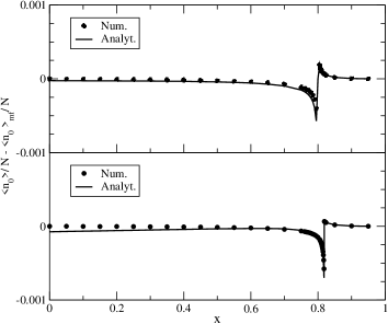
For the number of bosons, we compare the analytical formulae with the numerical results for the case of $\chi=-\sqrt{7}/2$ and $\chi=0$ in Fig. 4. In particular we are interested in the study of the $N^{0}$ corrections for the ground state, therefore we subtract the mean field contribution, $\langle n_{0}\rangle_{gs}^{mf}/N$, to both, analytical and numerical results. As expected we observe how the $N^{0}$ correction improve the description of $\langle n_{0}\rangle_{gs}$ specially near the critical point.

Figure 4: Variation of $(\langle n_{L=0}\rangle_{gs}-\langle n_{L=0}\rangle_{gs}^{mf})/N$ as a function of $x$ near the critical point for $L=0$. Full line is for the analytical and circles for are numerical results. Upper figure corresponds to $\chi=0$ and lower to $\chi=-\sqrt{7}/2$.

IV.2 The case $L=2$

For $L=2$, the numerical calculations have been carried out with an IBM code Isacker which has been modified for allowing calculations up to $N=100$ bosons. All numerical calculations for IBM presented below are performed for $N=100$.

For $L=2$ the case $\chi=0$ reduces to the $L=0$ situation already discussed. In particular, the analytical ground state energy is the same in both cases, although the $N^{0}$ correction differs; there exists only one kind of excitation: the $\beta$, while the $\mu=\pm 1$ and $\gamma$ excitations become spurious Goldstone bosons. The $\beta$ excitation energy is equivalent to (23). On the exact diagonalization side, the Hamiltonian (1) can be rewritten in terms of the generators of an $SU(1,1)$ algebra García-Ramos et al. (2005); Vidal et al. (2006) in the same way that in the $L=0$ case. Consequently, in this section we will only consider $L=2$ with $\chi\neq 0$. Any $\chi$ value can be analyzed but, as an illustration, here we will present results for the case $\chi=-\sqrt{7}/2$ that gives the $U(5)-SU(3)$ leg in the Casten triangle.

Figure 5: (Color online) Excitation energies (analytical), in arbitrary units, for one and two phonon states as a function of $x$ for $L=2$ and $\chi=-\sqrt{7}/2$.

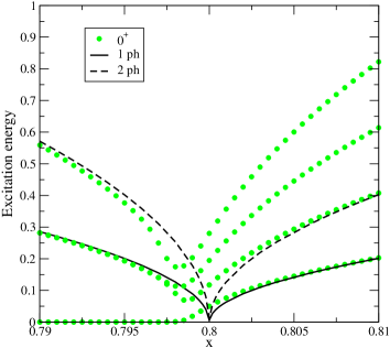
First, we plot the analytical results corresponding to one and two phonon excitations (Fig. 5). In the deformed phase, the bosons are $\beta$ and $\gamma$ excitations, while in the spherical phase they are spherical harmonic phonons. At the critical point the $\beta$ and the $\beta^{2}$ bands transform into one and two phonon bands, respectively. However, the $\gamma$, $\beta\gamma$, and $\gamma^{2}$ bands apparently disappear when entering in the spherical phase. Indeed, it happens because $\beta$ and $\gamma$ excitations become degenerate for $\beta=0$. The spherical phonon excitation is a five degenerate excitation where the deformed $\beta$ and $\gamma$ excitations collapse together with the Goldstone boson with projection $\pm 1$ (which is at zero energy in the deformed phase).

Figure 6: (Color online) Excitation energies (analytical and numerical), in arbitrary units, of one and two phonon states as a function of $x$ for $L=2$ and $\chi=-\sqrt{7}/2$ in the deformed phase. Lines correspond to analytical an dots to numerical results. The lowest $0^{+}$ state corresponds to $0^{+}_{2}$ and the $2^{+}$ states are respectively $2^{+}_{3}$ and $2^{+}_{5}$.

Figure 7: (Color online) Excitation energies (analytical and numerical), in arbitrary units, of one and two phonon states as a function of $x$ for $L=2$ and $\chi=-\sqrt{7}/2$ in the region around the critical point. The dots correspond to numerical results. The lowest $0^{+}$ state corresponds to $0^{+}_{2}$ and the lowest $2^{+}$ state corresponds to $2^{+}_{1}$.

Figure 8: (Color online) Excitation energies of one and two phonon states, in arbitrary units, as a function of $x$ for $L=2$ and $\chi=-\sqrt{7}/2$. Lines correspond to analytical an dots to numerical results.

In order to compare analytical and numerical results we will split the analysis in three different regions: deformed phase (Fig. 6), critical region (Fig. 7) and spherical phase (Fig. 8). The harmonic character of the results is observed in all these plots.

Figure 9: (Color online) $\langle n_{d}\rangle/N$ as a function of $x$ for $L=2$ and $\chi=-\sqrt{7}/2$, in the deformed phase for one phonon states. Lines correspond to analytical and dots to numerical results.

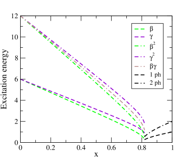
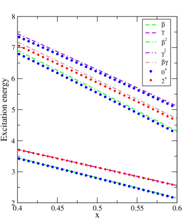
IV.2.1 Deformed phase

In the deformed phase (Fig. 6) one and two phonon excitations are clearly separated in energy. Note that the excitation energy for the $\gamma$ band is higher than the corresponding one for the $\beta$ band, although for $x=0$ ($SU(3)$ limit) they are degenerated. Also note that the $\gamma^{2}$ excitation carries the angular momentum projections $K=0,\pm 4$ which in this approach are degenerated.

Figure 10: (Color online) Excitation energies (numerical) of $2^{+}_{3}$ and $2^{+}_{4}$ states at the region of closest approach (see text) for $L=2$ and $\chi=-\sqrt{7}/2$.

The correspondence between numerical and analytical states is as follows: $\beta$ band is identified with $0^{+}_{2}$, $\gamma$ with $2^{+}_{3}$, $\beta^{2}$ with $0^{+}_{3}$, $\beta\gamma$ with $2^{+}_{5}$ and $\gamma^{2}$ with $0^{+}_{4}$. Note that the state $2^{+}_{2}$ belongs to the $\beta$ band, while $2^{+}_{4}$ to the $\beta^{2}$ band.

The overall agreement between analytical and numerical results is satisfactory and improves the description given in García-Ramos et al. (1998) for single and double phonon excitations, although in the present approach, no mixing between the different kind of excitations appear.

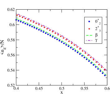
The average number of $d$ bosons in the deformed phase, normalized to the total number of bosons, is depicted in Fig. 9 for one phonon states (the results for two phonon states are not presented for clarity). It can be observed a smooth decrease of $\langle n_{d}\rangle$ when $x$ is increasing as it is expected when approaching the spherical phase.

Figure 11: (Color online) $\langle n_{d}\rangle/N$ (numerical) of $2^{+}_{3}$ and $2^{+}_{4}$ states at the region of closest approach (see text) for $L=2$ and $\chi=-\sqrt{7}/2$.

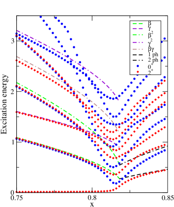
IV.2.2 Critical area

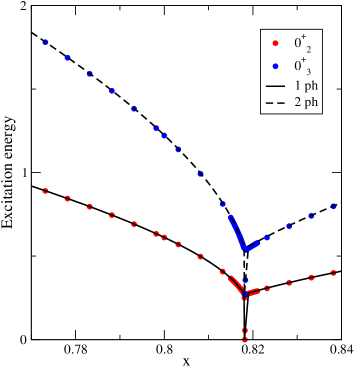
The comparison around the critical area (Fig. 7) becomes complicated because one and two phonon states have comparable energies and there appears interchange of character between states. For example at the critical point, the $\beta^{2}$ is at lower energy than the $\gamma$ excitation.

Starting at $x=0.75$ the correspondence between analytical and numerical states is similar to the one given in preceding section, but already at $x=0.8$ different states interchange its character. The correspondence between states is presented in table 1. From this table it is clear that there exists an interchange of character between the states corresponding to the $\gamma$, $\beta^{2}$, $\beta\gamma$, and $\gamma^{2}$ bands.

	$x=0.75$	$x=9/11$	$x=0.85$
$\beta$	$0^{+}_{2}$,$2^{+}_{2}$	$0^{+}_{2}$,$2^{+}_{2}$
$\gamma$	$2^{+}_{3}$	$2^{+}_{4}$
$\beta^{2}$	$0^{+}_{3}$,$2^{+}_{4}$	$0^{+}_{2}$,$2^{+}_{3}$
$\beta\gamma$	$2^{+}_{5}$	$2^{+}_{6}$
$\gamma^{2}$	$0^{+}_{5}$	$0^{+}_{7}$
$1$ phonon			$2^{+}_{1}$
$2$ phonons			$0^{+}_{2}$,$2^{+}_{2}$

Table 1: Correspondence between analytical and numerical states for three values of $x$: $x=0.75$ deformed phase, $x=9/11$ critical point and $0.75$ spherical phase. Only $0^{+}$ and $2^{+}$ states are indicated explicitly.

Figure 12: (Color online) $\langle n_{d}\rangle/N$ as a function of $x$, for $L=2$ and $\chi=-\sqrt{7}/2$, at the critical area for one phonon states. Lines correspond to analytical and dots to numerical results.

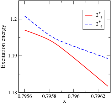
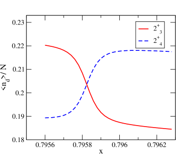
An interesting question that arises is if the interchange of character is due either to level crossing or to level repulsion. We have to take into account that the transition between $SU(3)$ and $U(5)$ is not an integrable path Arias et al. (2003b), i.e. a complete set of mutually commuting Hermitian operators does not exist. This implies that crossings are forbidden and only repulsion is allowed. In particular, in the thermodynamical limit the repulsion becomes anti-crossing, i.e. infinity repulsion. In Fig. 10 we show a zoom of one apparent crossing in Fig. 7 between $2^{+}$ states in the region around $x=0.796$, it is clearly seen that the levels indeed repel each other as expected. In order to illustrate this result and show how the two involved levels interchange their character, we present in Fig. 11 the expectation value of the $d$ boson number in both states. It is clearly observed that the states interchange their properties at the point of closest approach.

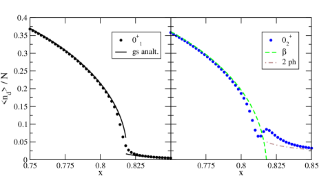
The average number of $d$ bosons, normalized to the total number of bosons, in the region around the critical point is depicted in Fig. 12 for the ground state (left panel) and for the $\beta$ band (right panel). One important feature is the discontinuity appearing at $x_{c}=9/11$ due to the existence of a first order phase transition. In the evolution of the $\beta$ band, it appears a kink in the numerical results at the critical point. This behavior at the critical point has been already observed for other observables such as isomer shifts Iachello and Zamfir (2004), derivative of the ratios of $4_{1}^{+}/2^{+}_{1}$ excitation energies Werner et al. (2002) or $B(E2:4^{+}_{1}\rightarrow 2^{+}_{1})/B(E2:2^{+}_{1}\rightarrow 0^{+}_{1})$ Rosensteel and Rowe (2005). Also note that the $0^{+}_{2}$ state transforms into a two phonon band when passing to the spherical phase.

Figure 13: (Color online) $\langle n_{d}\rangle/N$ as a function of $x$ for $L=2$ and $\chi=-\sqrt{7}/2$, in the spherical phase for one and two phonon states. Lines correspond to analytical and dots to numerical results.

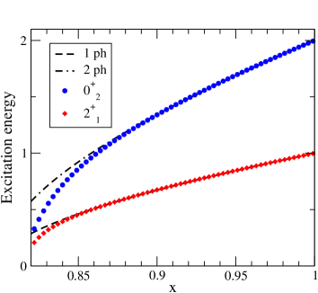
IV.2.3 Spherical phase

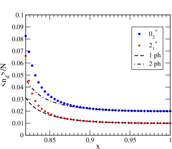
The last region of interest is the spherical phase (Fig. 8). Here, there exist a five degenerated phonon excitation. The correspondence between the analytical and the numerical results is clear: one phonon excitation corresponds to the state $2_{1}^{+}$ while two phonon excitation to the state $0_{2}^{+}$ (also to $2_{2}^{+}$ and $4_{1}^{+}$ states).

The average number of $d$ bosons, normalized to the total number of bosons, in the spherical region is depicted in Fig. 13 for the one and two phonon states. The main discrepancies between numerical and analytical results, as expected, appear close to the critical point. Note that the structure of the states is very simple and already for $x=0.9$ the number of $d$ bosons is fixed to $1$ and $2$ for one and two phonon states, respectively.

V Summary and conclusions

In this paper we have studied two–level boson models characterized by a lowest scalar $s$-boson and an excited $L$ boson through a Holstein-Primakoff transformation that allows to treat explicitly order by order a $N$ expansion. This treatment shows that only the leading $N$ term of the ground state energy is correct in a mean field (or Hartree-Bose) approach. We stress that the equilibrium nuclear shape corresponding to an IBM Hamiltonian should be obtained only considering the leading $N$ term of the ground state energy.

Depending on the value of $L$, models of interest in different fields can be obtained. Thus, $L=0$ is related to the Lipkin model first introduced in Nuclear Physics and then used in many fields, $L=1$ is the vibron model of interest in Molecular Physics, $L=2$ is the Interacting Boson Model of nuclear structure, etc. We have presented a method to go accurately beyond the standard mean field treatment so as to be able to compute finite size corrections to several spectroscopic observables. The model Hamiltonian used is a generalization for arbitrary $L$ of the Consistent Q Hamiltonian in the IBM. This Hamiltonian depends on two control parameters and changes in them allow to explore the full model space and the corresponding phase diagram. Although the formalism is general for any $L$ value, we have concentrated in the cases $L=2$ (IBM) and $L=0$. Both spherical and deformed phases have been studied with special emphasis in the gap for single and double excitations and the expectation values of the number of $L$ bosons in different states. Analytic results have been validated by comparison with full numerical calculations.