Isospin breaking in the vector current of the nucleon

Abstract

Extraction of the nucleon’s strange form factors from experimental data requires a quantitative understanding of the unavoidable contamination from isospin violation. A number of authors have addressed this issue during the past decade, and their work is reviewed here. The predictions from early models are largely consistent with recent results that rely as much as possible on input from QCD symmetries and related experimental data. The resulting bounds on isospin violation are sufficiently precise to be of value to on-going experimental and theoretical studies of the nucleon’s strange form factors.

1 Motivation

Isospin violation is generally a small effect. For example, consider the nucleon mass splitting, $(m_{n}-m_{p})/m_{p}=0.1\%$. One similarly expects isospin violation to have a small impact on the nucleon’s electromagnetic and weak form factors. However, this does not imply that isospin violation must be small relative to strangeness effects. To illustrate, recall that an explicit calculation in the electroweak theory leads to

$$G_{X}^{p,Z}(q^{2})=\hskip 190.63345pt$$

$$(1-4\sin^{2}\theta_{W})G_{X}^{p}(q^{2})-G_{X}^{n}(q^{2})-G_{X}^{s}(q^{2})-G_{X}^{u,d}(q^{2})\hskip 8.53581pt$$ (1)

for electric ($X=E$) and magnetic ($X=M$) form factors. Experimental studiesSAMPLE ; A4a ; A4b ; HAPPEXa ; HAPPEXb ; G0 show that the sum of the last two terms on the right-hand side is small. The size of isospin violation, $G_{X}^{u,d}(q^{2})$, relative to strangeness, $G_{X}^{s}(q^{2})$, is not obtained from these experiments.

In what follows, theoretical studies of $G_{X}^{u,d}(q^{2})$ will be reviewedDP ; Mi ; Ma ; LM ; KL . (Our entire discussion of isospin violation also fits within the more restrictive category called “charge symmetry breaking” and that language is used, for example, in Ref. Mi .) If the current understanding of these isospin violating effects is sufficiently precise, then the data from Refs. SAMPLE ; A4a ; A4b ; HAPPEXa ; HAPPEXb ; G0 allow for a determination of the authentic strange quark effects, $G_{X}^{s}(q^{2})$, which are of great interest to many people at present.

Independent of any chosen theoretical approach, each isospin violating form factor is simply the difference of isoscalar and isovector terms,

$$G_{X}^{u,d}(q^{2})\equiv G_{X}^{s\!\!\!/}(q^{2})-G_{X}^{v\!\!\!/}(q^{2})\,,$$ (2)

where $G_{X}^{s\!\!\!/}$ is obtained from

$$\left<p\left|\bar{u}\gamma_{\mu}u+\bar{d}\gamma_{\mu}d\right|p\right>-\left<n\left|\bar{u}\gamma_{\mu}u+\bar{d}\gamma_{\mu}d\right|n\right>$$ (3)

and $G_{X}^{v\!\!\!/}$ is obtained from

$$\left<p\left|\bar{u}\gamma_{\mu}u-\bar{d}\gamma_{\mu}d\right|p\right>+\left<n\left|\bar{u}\gamma_{\mu}u-\bar{d}\gamma_{\mu}d\right|n\right>$$ (4)

in a straightforward manner (see Refs. DP ; KL for details). Furthermore, we know that all isospin violation is ultimately a consequence of unequal quark masses, $m_{u}\neq m_{d}$, (“strong breaking”) and unequal quark electric charges, $e_{u}\neq e_{d}$ (“electromagnetic breaking”). The task for each theoretical approach is to determine the combinations of nucleon matrix elements shown in Eqs. (3) and (4), with both types of breaking included.

Since the sum of strangeness and isospin violation in Eq. (1) is measured to be a small fraction of the total form factors, and since isospin violation itself is expected to be a small fraction of the total form factors, it is reasonable to neglect contributions containing both strangeness and isospin violation as doubly (i.e. negligibly) small. This allows $G^{u,d}_{X}(q^{2})$ to be calculated without dynamical strange-quark effects. Such an approach is clearly advantageous for chiral perturbation theory, where addition of a dynamical strange quark leads to severe degradation of convergence properties of the chiral expansion. All of the theoretical studies to date have computed isospin violation without dynamical strange quarks.

Our discussion will be approximately chronological. The constituent quark model studies of Dmitrašinović and PollockDP and MillerMi , are discussed in Sec. 2, followed by Ma’s use of a light-cone meson-baryon fluctuation modelMa in Sec. 3. The constraints of chiral symmetry are discussed in Sec. 4, based on a collaboration with MobedLM using chiral perturbation theory. Section 5 reviews the recent results from work with KubisKL that combines chiral perturbation theory with resonance saturation and information from dispersion analyses. The final section, Sec. 6, provides a brief summary.

2 Constituent quark model

In a constituent quark model, we might expect the scale of strong breaking to be set by constituent quark masses, which the authors of Ref. DP take to be $(m_{D}-m_{U})/m_{Q}\sim 1.2\%$, and the scale of electromagnetic breaking to be set by $\alpha\sim 0.7\%$. To do better than this order-of-magnitude guess, an explicit calculation is required.

The first calculation was carried out by Dmitrašinović and PollockDP using oscillator confinement and a Coulomb potential,

$$H = H_{0}+V_{EM}\,,$$ (5)

$$H_{0} = \sum_{i=1}^{3}\frac{{\bf p}_{i}^{2}}{2m_{i}}+\frac{k}{2}\sum_{i<j}^{3}({\bf r}_{i}-{\bf r}_{j})^{2}\,,$$ (6)

$$V_{EM} = \sum_{i<j}^{3}\frac{e_{i}e_{j}}{4\pi\left|{\bf r}_{i}-{\bf r}_{j}\right|}\,.$$ (7)

Recall that this choice for $H_{0}$ produces Gaussian spatial wave functions. With parameters fixed to be $m_{Q}=330$ MeV, $m_{D}-m_{U}=4$ MeV, and $k$ determined from the experimental mass difference between $\Delta(1232)$ and nucleon, Ref. DP finds

$$G_{M}^{s\!\!\!/}(0)=G_{M}^{v\!\!\!/}(0) = \frac{1}{3}\left[\frac{m_{D}}{m_{U}}-\frac{m_{U}}{m_{D}}\right]\approx 0.008\,,$$ (8)

$$G_{M}^{u,d}(0) = G_{M}^{s\!\!\!/}(0)-G_{M}^{v\!\!\!/}(0)=0\,,$$ (9)

$$\frac{\delta\left<r_{E}^{2}\right>}{\left<r_{E}^{2}\right>} = 1.1\%\,,$$ (10)

$$\frac{\delta\left<r_{M}^{2}\right>}{\left<r_{M}^{2}\right>} = 0.4\%\,,$$ (11)

where $r_{X}^{2}$ denotes a squared radius as usual. These estimates are compatible with our order-of-magnitude guesses, but what confidence level should be assigned to the precise values?

Here is a list of some limitations of this model (all of which are mentioned explicitly in Ref. DP ):

• The chosen parameters lead to, $m_{n}-m_{p}=3$ MeV, 230% above experiment.

• The nucleon charge radius, $\sqrt{\left<r_{E}^{2}\right>}=0.62$ fm, is 30% below experiment.

• Gaussian spatial wave functions cause both $G_{E}(q^{2})$ and $G_{M}(q^{2})$ to be unrealistic at large ${\bf q}^{2}$.

• The strong hyperfine interaction is omitted.

• Chiral symmetry is absent.

In Section IV B of Ref. DP , the authors conclude, “…we may expect to have calculated the correct sign and order of magnitude of the effects of interest.”

Subsequently, MillerMi used a more complete constituent quark model and explicitly addressed each of the limitations listed above, except chiral symmetry. (Miller says chiral symmetry is implicit in the charge symmetry conserving pion cloud of this modelprivate .) His Hamiltonian is

$$H = K+V_{\rm con}+V_{\rm em}+V_{g}\,,\hskip 113.81102pt$$ (12)

$$K = \sum_{i=1}^{3}\left(m_{i}+\frac{p_{i}^{2}}{2m_{i}}\right)\,,$$ (13)

$$V_{\rm em}=\alpha\sum_{i<j}q_{i}q_{j}\left(\frac{1}{r_{ij}}-\frac{\pi}{2}\delta(\vec{r}_{ij})\left[\frac{2}{\bar{m}^{2}}+\frac{4}{3}\frac{\vec{\sigma}(i)\cdot\vec{\sigma}(j)}{\bar{m}^{2}}\right]\right)\,,$$ (14)

$$V_{g}=-\alpha_{s}\!\!\sum_{i<j}\lambda_{i}\cdot\lambda_{j}\!\!\left[\frac{\pi}{2}\delta(\vec{r}_{ij})\!\left(\frac{1}{m_{i}^{2}}+\frac{1}{m_{j}^{2}}+\frac{4}{3}\frac{\vec{\sigma}(i)\cdot\vec{\sigma}(j)}{m_{i}m_{j}}\right)\right]\!.$$ (15)

Two options for $V_{\rm con}$ are studied; one gives Gaussian form factors,

$$\Psi(\rho,\lambda) = N\exp{\left(\frac{\rho^{2}+\lambda^{2}}{-2\beta}\right)}\,,$$ (16)

$$\vec{\rho} = \frac{1}{\sqrt{2}}(\vec{r}_{1}-\vec{r}_{2})\,,$$ (17)

$$\vec{\lambda} = \frac{1}{\sqrt{6}}(\vec{r}_{1}+\vec{r}_{2}-2\vec{r}_{3})\,,$$ (18)

and the other gives power-law form factors,

$$\Psi^{2}(R)=\frac{2\sqrt{6}\Lambda^{7}}{\pi^{3}6^{5}}RK_{1}\left(\sqrt{\frac{2}{3}}\Lambda R\right)\,,$$

$$\Rightarrow G_{E}(Q^{2})=\left(\frac{\Lambda^{2}}{Q^{2}+\Lambda^{2}}\right)^{4}\,.$$ (19)

For the Gaussian case, Ref. Mi uses the experimental proton magnetic moment to determine $\bar{m}=337$ MeV, the experimental $m_{\Delta}-m_{N}$ value to fix $\alpha_{s}$ as a function of $\beta$, and then considers three choices for $\beta$ which define three models as shown in Table 1.

Table 1: Parameter values for the three Gaussian models of Ref. Mi .

Model	1	2	3
$\sqrt{\beta}$ (fm)	0.7	0.6	0.5
$\alpha_{s}$	2.3	1.2	0.35
$m_{D}-m_{U}$ (MeV)	5.2	3.8	2.3

Figures 4, 5, 6 and 7 of Ref. Mi display the resulting effects of isospin violation on $G_{E}(q^{2})$ and $G_{M}(q^{2})$, including the separate contributions from $K$, $V_{\rm em}$ and $V_{g}$. In each case, the isospin violating contributions vanish for $q^{2}=0$, and are less than 0.2% in magnitude for a momentum transfer of 0.1 GeV². For power-law form factors, Ref. Mi obtains $\Lambda=5.90$/fm from the experimental value of $\left<r_{E}^{2}\right>$, and all isospin violating effects remain small.

The combined work of Refs. DP ; Mi provides an excellent understanding of isospin violation within the constituent quark model, but we must now ask which features of the results are a true reflection of nature, and which are model-dependent. For example, there are symmetries in these quark models that lead to $G_{M}^{u,d}(0)=0$, recall Eq. (9), but, as we’ll see in Sec. 4, this is not a symmetry of nature. It is therefore interesting to explore other theoretical approaches as well.

3 Light-cone meson-baryon fluctuation model

To discuss the method used by MaMa , we must think at the hadron level rather than the constituent quark level. Fluctuations of a nucleon into a virtual pion-nucleon pair, $p\to\pi^{+}n$ and $n\to\pi^{-}p$, occur commonly. As always, isospin violation arises from strong breaking (at the hadron level, this means $m_{n}-m_{p}\neq 0$) and from electromagnetic breaking (which now means the Coulomb attraction of a charged/charged $\pi^{-}p$ pair is different from the charged/neutral $\pi^{+}n$ pair). The expression for isospin violation in the magnetic form factor at vanishing momentum transfer, is

$$G_{M}^{u,d}(0)=\bigg{(}P(n\to\pi^{-}p)-P(p\to\pi^{+}n)\bigg{)}\bigg{(}\mu^{n}_{\pi^{-}p}-\mu_{n}\bigg{)}\,,$$ (20)

where $P()$ denotes a fluctuation probability, and $\mu^{n}_{\pi^{-}p}$ is the magnetic moment for the neutron’s fluctuation.

To determine $\mu_{\pi^{-}p}^{n}$, begin with the fact that total angular momentum is orbital angular momentum plus proton spin,

$$\left|\frac{1}{2},\frac{1}{2}\right>_{J}=\sqrt{\frac{2}{3}}\bigg{|}1,1\bigg{>}_{L}\left|\frac{1}{2},-\frac{1}{2}\right>_{S}-\sqrt{\frac{1}{3}}\bigg{|}1,0\bigg{>}_{L}\left|\frac{1}{2},\frac{1}{2}\right>_{S}\,.$$ (21)

This leads directly to

$$\mu_{\pi^{-}p}^{n} = -\frac{\mu_{p}}{3}+\frac{\mu_{n}}{3}\left(\frac{2m_{n}}{m_{\pi^{-}}+m_{p}}\right)\left(\frac{m_{\pi^{-}}}{m_{p}}-\frac{m_{p}}{m_{\pi^{-}}}\right)$$ (22)

$$= -4.75~{}~{}~{}~{}~{}~{}\Rightarrow~{}~{}~{}~{}~{}~{}\mu_{\pi^{-}p}^{n}-\mu_{n}=-2.84\,.$$

To determine the difference of fluctuation probabilities needed for Eq. (20), a light-cone Gaussian wave function is used,

$$\psi=Ae^{-({\cal M}^{2}-m_{N}^{2})/(8\alpha^{2})}\,,$$ (23)

where

$${\cal M}^{2}=\sum_{i=1}^{2}\frac{{\bf k}_{\perp\,i}^{2}+m_{i}^{2}}{x_{i}}$$ (24)

is the invariant mass of the meson-baryon state. (Note the implicit assumption that $A$ is independent of which nucleon is fluctuating; Ref. Ma points out that this assumption is not required, but the uncertainties associated with relaxing it are difficult to estimate.) From the experimental Gottfried sum rule, one finds

$$P(p\to\pi^{+}n)\approx P(n\to\pi^{-}p)\approx 0.15\,.$$ (25)

The final remaining parameter is the radius, $\alpha$, and it leads to a large uncertainty. Ref. Ma uses two bounds,

$$\alpha=300{\rm MeV}~{}~{}~{}\Rightarrow~{}~{}~{}P(n=\pi^{-}n)-P(p=\pi^{+}n)=0.2\%\,,$$ (26)

and

$$\left.\begin{array}[]{l}\alpha(n\to\pi^{-}p)=205{\rm MeV}\\ \alpha(p\to\pi^{+}n)=200{\rm MeV}\end{array}\right\}$$

$$\Rightarrow~{}~{}~{}P(n=\pi^{-}n)-P(p=\pi^{+}n)=3\%\,,$$

to arrive at

$$G_{M}^{u,d}(0)\approx 0.006\to 0.088\,.$$ (31)

However, Miller suggests that (205-200)/200=2.5% is too large for a Coulomb effect, and states: “A reasonable estimate of the effect could be 0.03 nuclear magnetons.”Mi .

Thus, the light-cone meson-baryon fluctuation model provides an explicit example of a model that does not lead to $G_{M}^{u,d}(0)=0$. In particular, this model predicts $G_{M}^{u,d}(0)>0$.

4 Chiral perturbation theory

Chiral perturbation theory is not a model; it merely administrates the global symmetries of QCD. This has the advantage of retaining no model dependence in predictions, and it has the disadvantage that quantities not determined by global symmetries remain completely unknown. In Ref. LM , isospin violation in the nucleon’s vector form factors is studied within chiral perturbation theory to leading order for the electric case, and to next-to-leading order for the magnetic case.

Because isospin violation arises from both strong breaking and electromagnetic breaking, our chiral perturbation theory must include dynamical photons as well as dynamical pions. A single baryon will flow through the process, though its identity may change from proton to neutron or even to $\Delta(1232)$ by absorbing or emitting a pion (recall the fluctuations discussed in Sec. 3). Ref. LM uses the formalism of heavy baryon chiral perturbation theoryJM ; BKM , and the perturbative expansion is defined in powers of electric charge $e$, momentum $q/\Lambda$, pion mass $m_{\pi}/\Lambda$, and mass difference $(m_{\Delta}-m_{N})/\Lambda$, where $\Lambda$ denotes either $4\pi F_{\pi}$ or $m_{N}$. Writing the Lagrangian in standard notation,

$${\cal L}_{\rm ChPT}={\cal L}^{(1)}+{\cal L}^{(2)}+{\cal L}^{(3)}+{\cal L}^{(4)}+{\cal L}^{(5)}+\ldots\,,$$ (32)

Ref. LM shows that the isospin violating form factors begin in ${\cal L}^{(4)}$ (plus the corresponding loop diagrams), and next-to-leading effects are in ${\cal L}^{(5)}$ (plus the corresponding loop diagrams). For a general observable at this high order, two-loop diagrams routinely appear and the most general effective Lagrangian contains literally hundreds of low-energy constants (i.e. parameters whose numerical values are not constrained by global symmetries, and hence unknown to chiral perturbation theory).

For the specific case of $G_{M}^{u,d}(q^{2})$, Ref. LM shows that the situation is much simpler than for a general observable due to five key observations:

• $G_{M}^{u,d}(q^{2})$ receives no two-loop contributions up to next-to-leading order. (In particular, “photon+photon” loop diagrams lack the required spin operators, “photon+ pion” loop diagrams sum to anticommutators of Pauli-Lubanski operators, and “pion+pion” loop diagrams have only higher-order isospin violation.)

• All one-loop photon effects in $G_{M}^{u,d}(q^{2})$ can be absorbed into the physical value of $m_{n}-m_{p}$.

• Explicit $\Delta(1232)$ effects are found, numerically, to be smaller than systematic uncertainties.

• $G_{M}^{u,d}(q^{2})$ contains just one combination of low-energy constants at leading order — it’s a simple additive constant — and no additional low-energy constants at next-to-leading order. (The fact that no global symmetry forces this constant to vanish is not realized in some constituent quark models, as discussed in Sec. 2.)

• All isospin breaking in loops, up to next-to-leading order, is ultimately due to $m_{n}-m_{p}$.

Based on these observations, a parameter-free prediction for the difference $G_{M}^{u,d}(q^{2})-G_{M}^{u,d}(0)$ is obtained in Ref. LM .

Isospin violation in the electric form factor is discussed in Ref. MENU99 , but only to leading order because in this case there are two-loop contributions and additional unknown constants at next-to-leading order.

Though it is useful to have these “pion cloud contributions” computed within chiral perturbation theory, the missing combination of low-energy constants indicates that chiral perturbation theory alone will not meet all of our goals, and we must turn our attention to a method for understanding the physics that resides within the low-energy constants.

5 Chiral perturbation theory with resonance saturation

The chiral perturbation theory calculations of Ref. LM were reproduced in Ref. KL using two separate formalisms: a repeat of the heavy baryon calculation, and a newer method known as infrared regularizationBL . This newer approach is simpler to manage and needs fewer Feynman diagrams, but physical results must be identical. Ref. KL finds and corrects some errant factors of 2 in Ref. LM , and confirms all of the features mentioned in Sec. 4.

With the results of chiral perturbation theory now firmly in hand, Ref. KL addresses the issue of unknown low-energy constants. They are not constrained by chiral symmetry, nor by any other global symmetry of QCD. Since chiral perturbation theory is the low-energy effective theory of QCD, where pions (and in our case, photons too) are dynamical, the low-energy constants must account for all of the higher-energy QCD dynamics. Most important would be the exchange of the lightest resonances that are too heavy to appear explicitly in the effective theory: for vector form factors, these are the $\rho$ and $\omega$. Figure 1 sketches this notion of resonance saturation.

Figure 1: The basic idea of resonance saturation for a nucleon’s vector form factor.

Mathematically, it is easy to see that the exchange of a heavy particle is a low-energy constant at leading order,

$${\rm propagator}\sim\frac{1}{M^{2}-q^{2}}=\frac{1}{M^{2}}+O\left(\frac{q^{2}}{M^{2}}\right)\,.$$ (33)

Of course these resonances have to be coupled in a way consistent with chiral symmetry.

This type of resonance saturation was shown long ago to work very well in the meson chiral Lagrangianressat1 ; ressat2 ; ressat3 , though it has been shown that the nucleon’s vector form factors require inclusion of extra resonances beyond merely the $\rho$ and $\omega$KM . Nevertheless, our present goal is only to compute the isospin violating pieces of these form factors; they come from $\rho-\omega$ mixing, and Ref. KL points out that any effects of higher resonances are more severely suppressed in this case.

The contributions of resonance saturation to the isospin violating form factors are shown diagrammatically in Fig. 2.

Figure 2: Resonance saturation contributions to isospin violation in the nucleon’s vector form factors.

The corresponding equations are

$$\delta G_{E}^{u,d}(q^{2}) = \frac{\Theta_{\rho\omega}}{M_{V}(M_{V}^{2}-q^{2})^{2}}\left[\left(1+\frac{\kappa_{\omega}M_{V}^{2}}{4m_{N}^{2}}\right)g_{\omega}F_{\rho}q^{2}\right.$$ (34)

$$\left.-\left(1+\frac{\kappa_{\rho}M_{V}^{2}}{4m_{N}^{2}}\right)g_{\rho}F_{\omega}q^{2}\right]\,,$$

$$\delta G_{M}^{u,d}(q^{2}) = \frac{\Theta_{\rho\omega}}{M_{V}(M_{V}^{2}-q^{2})^{2}}\left[\left(q^{2}+\kappa_{\omega}M_{V}^{2}\right)g_{\omega}F_{\rho}\right.$$ (35)

$$\left.-\left(q^{2}+\kappa_{\rho}M_{V}^{2}\right)g_{\rho}F_{\omega}\right]\,,$$

where $M_{V}$, $F_{\rho}$ and $F_{\omega}$ are the vector meson mass and decay constants, and the $\rho-\omega$ mixing parameter has been determined from experimental masses and branching ratios to beKucM

$$\Theta_{\rho\omega}=(-3.75\pm 0.36)\times 10^{-3}{\rm GeV}^{-2}\,.$$ (36)

If we had numerical values for the couplings of vector mesons to nucleons, $g_{\rho}$, $\kappa_{\rho}$, $g_{\omega}$ and $\kappa_{\omega}$, then Eq. (35) could be expanded in powers of $q^{2}$ to obtain the desired low-energy constant (at $q^{2}=0$) as well as additional contributions that are technically of higher order in the chiral expansion. We immediately see that Eq. (34) vanishes at $q^{2}=0$ as required by global symmetries, but nonzero contributions from higher orders in the chiral expansion would be obtained.

Figure 3: Isospin violation in the electromagnetic form factors, as obtained from Ref. KL .

In principle, there is a wide assortment of techniques for attempting to quantify $g_{\rho}$, $\kappa_{\rho}$, $g_{\omega}$ and $\kappa_{\omega}$, but finding an approach with rigorously-quantifiable uncertainties is difficult. In an attempt to rely as directly as possible on experimental data rather than models, Ref. KL uses values extracted from dispersive analyses of nucleon electromagnetic form factors. For the $\rho$ couplings, these analyses must account for the non-resonant two-pion continuum in addition to the Breit-Wigner $\rho$ resonance. Data from Refs. MMD ; BHM lead to the ranges

$$4.0< g_{\rho} <6.2\,,$$ (37)

$$5.1< \kappa_{\rho} <6.8\,.$$ (38)

For the $\omega$ couplings, it is sufficient to consider only pure zero-width resonance pole residues, and Refs. MMD ; HM ; BHM2 produce the ranges

$$41.8< g_{\omega} <43.0\,,$$ (39)

$$-0.16< \kappa_{\omega} <0.57\,.$$ (40)

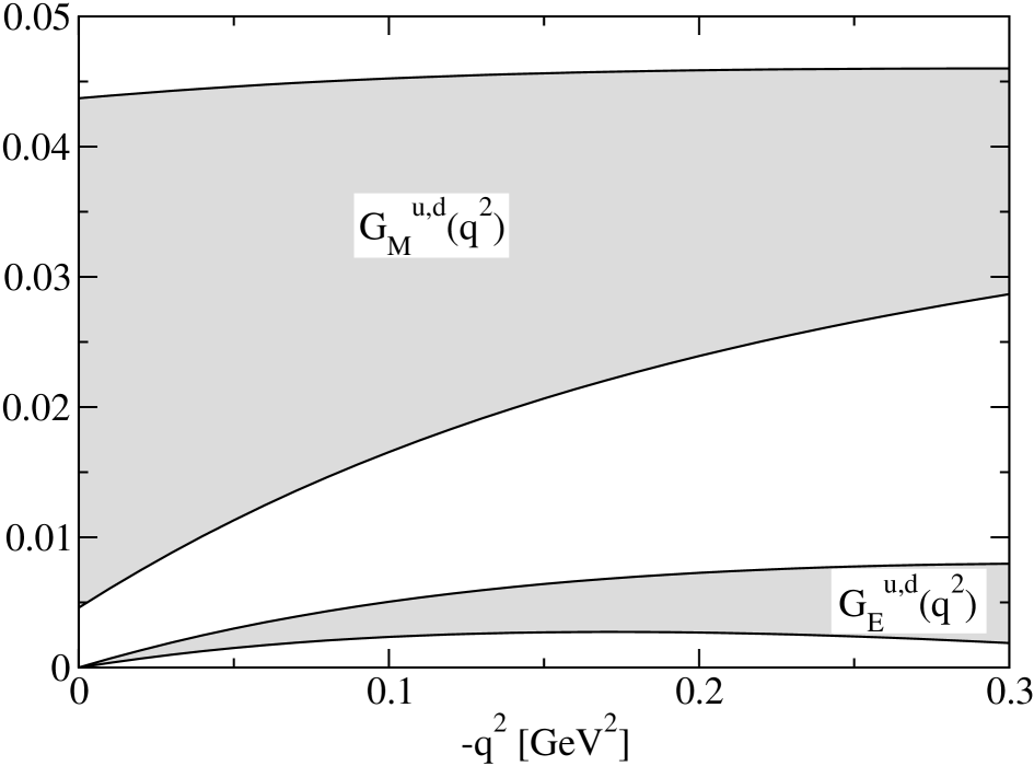
The final results of Ref. KL , reproduced in Fig. 3, include the worst-case errors bars obtained from spanning the ranges in Eqs. (37-40) above; the poorly-known $\kappa_{\omega}$ dominates the uncertainties. Notice that the range of $G_{M}^{u,d}(0)$ does not include zero, while $G_{E}^{u,d}(0)=0$ is required. Both form factors are positive over the momentum range considered.

6 Summary

Early studies of isospin violation in the nucleon’s vector form factors led to a clear understanding within specific quark models. Use of chiral perturbation theory avoids all model dependence, but leaves some parameters undetermined. Phenomenologically, those parameters are saturated by resonances, and numerical values are obtained with minimal model-dependence by using dispersive analyses. The results in Fig. 3 represent a conservative determination of isospin violation, as obtained from worst-case error bars.

Because it is the sum $G_{X}^{s}(q^{2})+G_{X}^{u,d}(q^{2})$ from Eq. (1) that is measured in experiments, Fig. 3 provides a theoretical error bar for the extraction of $G_{X}^{s}(q^{2})$. As shown explicitly in Table III of Ref. KL , modern experiments are already approaching this level of precision.

References

- (1) D. T. Spayde et al. (SAMPLE), Phys. Lett. B583, 79 (2004).
- (2) F. E. Maas et al. (A4), Phys. Rev. Lett. 93, 022002 (2004).
- (3) F. E. Maas et al., Phys. Rev. Lett. 94, 152001 (2005).
- (4) K. A. Aniol et al. (HAPPEX), Phys. Rev. Lett. 96, 022003 (2006).
- (5) K. A. Aniol et al. (HAPPEX), Phys. Lett. B635, 275 (2006).
- (6) D. S. Armstrong et al. (G0), Phys. Rev. Lett. 95, 092001 (2005).
- (7) V. Dmitrašinović and S. J. Pollock, Phys. Rev. C52, 1061 (1995).
- (8) G. A. Miller, Phys. Rev. C57, 1492 (1998).
- (9) B.-Q. Ma, Phys. Lett. B408, 387 (1997).
- (10) R. Lewis and N. Mobed, Phys. Rev. D59, 073002 (1999).
- (11) B. Kubis and R. Lewis, Phys. Rev. C74, 015204 (2006).
- (12) G. A. Miller, private communication.
- (13) E. Jenkins and A. V. Manohar, Phys. Lett. B255, 558 (1991).
- (14) V. Bernard, N. Kaiser and U.-G. Meißner, Int. J. Mod. Phys. E4, 193 (1995).
- (15) R. Lewis and N. Mobed, PiN Newslett. 15, 144 (1999).
- (16) T. Becher and H. Leutwyler, Eur. Phys. J. C9, 643 (1999).
- (17) G. Ecker, J. Gasser, A. Pich and E. de Rafael, Nucl. Phys. B321, 311 (1989).
- (18) G. Ecker, J. Gasser, H. Leutwyler, A. Pich and E. de Rafael, Phys. Lett. B223, 425 (1989).
- (19) J. F. Donoghue, C. Ramirez and G. Valencia, Phys. Rev. D39, 1947 (1989).
- (20) B. Kubis and U.-G. Meißner, Nucl. Phys. A679, 698 (2001).
- (21) A. Kucurkarslan and U.-G. Meißner, Mod. Phys. Lett. A21, 1423 (2006).
- (22) P. Mergell, U.-G. Meißner, Eur. Phys. J. A20, 469 (2004).
- (23) M. A. Belushkin, H.-W. Hammer and U.-G. Meißner, Phys. Lett. B633, 507 (2006).
- (24) H.-W. Hammer and U.-G. Meißner, Eur. Phys. J. A20, 469 (2004).
- (25) M. A. Belushkin, H.-W. Hammer and U.-G. Meißner, hep-ph/0608337. (Ref. KL used preliminary results.)