address=Departament de Estructura i Constituents de la Materia,
Diagonal 647, Universitat de Barcelona, 08028 Spain
Phenomenological hadron form factors: shape and relativity
Abstract
The use of relativistic quark models with simple parametric wave functions for the understanding of the electromagnetic structure of nucleons together with their electromagnetic transition to resonances is discussed. The implications of relativity in the different ways it can be implemented in a simple model are studied together with the role played by mixed symmetry s-state and D-state deformations of the rest frame wave functions of the nucleon and resonance.
Keywords:
relativistic quark models, nucleon form factors, nucleon-delta transition:
12.39.Ki, 14.20.Gk, 13.40.Gp, 14.20.Dh1 Introduction
Understanding the structure of hadrons from the underlying theory of the strong interaction, QCD, has proved to be a quite demanding task from the theoretical point of view. The most promising approach which claims to have more solid connections to the theory is lattice-QCD where the electromagnetic structure of hadrons is beginning to be unveiled as the computational power keeps increasing.
We are confronted during the last years with a very interesting situation: experiments keep improving precision on hadronic observables and also keep providing finer and finer databases for electromagnetic observables, both for elastic processes and for transitions. As of today, we are not able to compute those observables from QCD and are still far from being able to do so in a well grounded lattice-QCD computation. Thus it becomes necessary to resort to models which should enable us to get a partial understanding of the processes at hand and which should above all serve to guide experiments.
Quark models are an ideal tool for that purpose, they incorporate part of the symmetries and the degrees of freedom of the original problem and permit to analyze the importance of some of them, namely the relevance of relativity and of the different configurations in the rest frame wave functions. The use of quark models to study electromagnetic form factors of nucleons and transitions to resonances has some history to which we cannot do justice in these proceedings. The reader may check Refs. Chung ; simula ; Eli ; boffi ; mauro ; julia04 and references therein if he is interested in following the quark model path along these last years. Many of the fine details of the results shown here are given in Refs. julia04 ; dstate .
The contribution is organized as follows, in the next section a formal description of the quark model and of the way electromagnetic form factors are extracted from matrix elements of the electromagnetic current is given for the elastic case. Then in section III the elastic electromagnetic form factors are considered and explored in detail. Section IV is devoted to the transition to the resonance, exploring the effect of D-state configuration on the rest frame wave functions, Section V contains a final summary and discussion.
2 The baryon model
A simple way to build a descriptive phenomenological model is by constructing a mass operator in its spectral representation, being the different states of the representation the physical states. The ground state wave functions are built with a set of parameters which can be fitted to reproduce part of the known experimental data. This approach, in a more rigorous rendition, is explained in Ref. julia04 .
Considering the , and , their wave functions are constructed in the SU(6) symmetric quark model. The is built as the ground state, the as the spin-flip excitation of the ground state, and the as a radial excitation. This assumption is of course restrictive with respect to further components in the wave functions. The main improvement to these is the consideration of components. This is out of the scope of this contribution, advances in this direction have been reported in Ref. RiskaLi .
Those symmetric components can be written as:
| (1) |
where , , , and stand for spatial, color, spin and flavor respectively. Other symmetry components which we will consider are mixed symmetry s-state ones, written as:
| (2) |
and state ones, which for the nucleon and the read:
| (3) |
The spin-flavor components are written explicitly:
| (4) | |||||
| (5) | |||||
| (6) |
and the spatial wave functions are written in momentum space as:
| (7) | |||||
| (8) |
using the following momenta for the three quark system: , and The radial ground state wave function contains 2 parameters, which are fixed together with the constituent quark mass to reproduce the magnetic form factor of the proton in each of the forms of kinematics, which will be shown in the following section. The parameter values obtained for each of the forms are given in Table 1.
| (MeV) | (MeV) | (fm) | ||
|---|---|---|---|---|
| point form | 350 | 640 | 9/4 | 0.19 |
| front form | 250 | 500 | 4 | 0.55 |
| instant form | 140 | 600 | 6 | 0.63 |
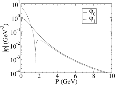
The spatial wave function of the first radial excitation is given explicitly in Ref. julia04 . It is constructed from the ground state one by imposing both orthogonality and the presence of a node in a simple way. In Fig. 1 the ground state () and first radial excitation () are plotted.
2.1 Relativity and quark currents
From a practical point of view, and due to the space constraints of these proceedings, let us explain in words the use of the different forms of relativistic kinematics. The main reason why relativity needs to be accounted for can be seen in a rough estimate of the quark velocity inside a proton. Once this is agreed there are in the literature three main ways of building relativity into a hamiltonian formalism, first discussed by Dirac dirac and later well developed in Refs. polyzou ; coe92 . In a non rigorous way which is well suited for explaining our procedure let us present the following rendition of the different forms.
The three forms differ among themselves in the kinematical group of the Poincarè group, that is, the subgroup whose commutator relations are not affected by the interactions. According to this classification we have: instant form, where the subgroup is made of rotations and translations at a fixed time, point form, where boosts and rotations are kinematic, and front form, where, for example, boosts along the light cone are kinematical.
For each form of kinematics the dynamics generates the current-density operator from a kinematic current, which is specified by the expression:
| (9) |
in the case of Lorentz kinematics, and:
| (10) | |||
| (11) |
for light-front kinematics and finally by:
| (12) |
for instant kinematics. and are initial and final momenta of quark . and are initial and final velocities of quark respectively. In each case only covariance under the kinematic subgroup is required.
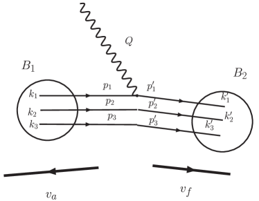
In Fig. 2 the role played by the form of kinematics which relates the variables at rest and the ones at the vertex is pictured graphically. These relations between both the rest frame spins and momenta to those of the moving frame depend on the form at use, their explicit formulae are given in Ref. julia04 . Here it suffices to be aware that in those relations is where the relativistic nature of the computation enters.
3 Nucleon form factors
The cross section for the elastic electron-nucleon scattering may be written in terms of two form factors. In the literature there are two usual sets, Pauli and Dirac form factors, and or Sachs form factors, and . Both sets are related by kinematical factors.
The elastic form factors can be extracted from the electromagnetic current taking appropriate matrix elements of spin states. They can be defined through the following matrix elements of the current operator for the case of instant and point form:
| (13) |
with .
In the front form case, the form factors are extracted from matrix elements of the component of the current, defined as :
| (14) |
As an explicit example, one can evaluate the matrix elements of Eq. (13) with the antisymmetric nucleon wave function and the quark current (9) multiplied by 3 (the number of constituent quarks). After summing over spin and isospin indices we arrive to the explicit expressions of the form factors in instant and point form:
| (15) | |||||
| (18) |
The Jacobian factor ,
| (20) |
where are given explicitly in Ref. julia04 . The jacobians differ in instant and point form.
The coefficient is determined by the spectator Wigner rotations:
| (21) | |||||
| (23) |
The boost velocities , are , in point form and , with instant kinematics. is defined as . The corresponding expressions for front form kinematics can be obtained using the explicit Melosh rotations given in Ref. julia04 .
3.1 Numerical results
The three parameters of the model in each of the forms of kinematics are fitted to achieve a good reproduction of both the dependence of the magnetic form factor of the proton and of its magnetic moment. The three forms accommodate the experimental data for the form factor and the pursued agreement is found with each of them. This was not guaranteed as we cannot assess apriori the importance of higher contributions, such as exchange currents, which may in each of the forms have a different relative importance. This happens for example when studying the form factor of a quark-antiquark pair which are bound to form a low mass system, e.g. a pion, there the point form has been proved to be unable to get close to the data desplanques ; junheplb ; junheepja .
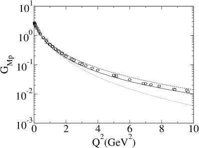
The description of the magnetic form factor can be seen in Fig. 3. The low domain is essentially well reproduced irrespective of the form at use. The high data, on the contrary is better understood when instant and front form are considered, point form underestimates the experimental data above 3 GeV2. This behavior at high was already reported by the Graz group boffi .
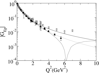
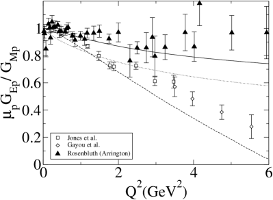
Once the parameters are fixed in each of the forms the remaining form factors of the nucleon were explored. The electric form factor of the proton is plotted in Fig. 3. At low all forms reproduce the experimental data, giving an accurate description of the charge radius of the proton, given in Table 2. This fall-off at low is in fact very close to the magnetic form factor one, both approximately dropping as the standard dipole. The differences found in this form factor above 3 GeV2 are already quite interesting as can be seen in the figure. First of all, an abrupt qualitative difference among the forms can be noticed, while point and instant forms remain positive up to GeV2 in front form the electric form factor of the proton becomes negative at around 6 GeV2. This was already in the light-front computations of Chung and Coester Chung although there and are plotted instead of and . This would be mostly anecdotical if it was not from the fact that the recent form factor data measured at JLAB using polarization transfer techniques exhibit a similar trend jones . The expected zero crossing appearing at 7.5 GeV2 arrington .
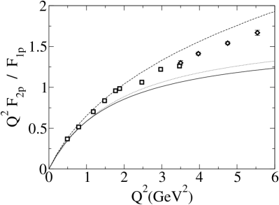
This dependence of the electric form factor, the accessible quantity is in fact the ratio , was not expected in the first pQCD predictions where it was believed that the ratio would be flat at high enough . The new experimental data however would rather be closer to . In Fig. 4 both the ratio and are depicted for the three different forms as compared to the new data. As before (this is nothing more than a different view at the same information contained in and ) front form gets closer to the high- tendency of the data.
Finally the values for the magnetic moments and proton charge radii are given in Table 2. Instant and Front form get values for the magnetic moments which are in close agreement with the experimental data, while point form underestimates the value by 10 %.
3.2 Electromagnetic form factors of the neutron: mixed symmetry components
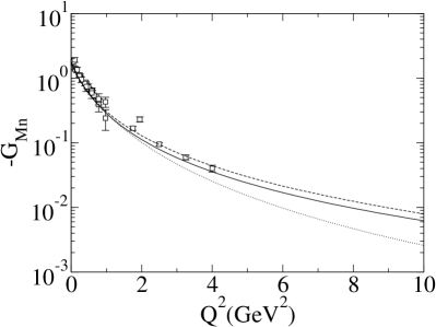
The neutron magnetic form factor comes out mostly in agreement with the experimental data as can be seen in Fig. 5. Similar features as for the proton case are found, instant and front forms provide similar descriptions in the considered domain while point form tends to predict a lower value at high .
The neutron magnetic moment is given in table 2. The values are in all cases smaller (in magnitude) than the experimental value, with point form giving the poorest number. In front form, the value is better but is still 10% off. This is similar to what was found in Ref. Chung . There the possibility of anomalous magnetic moments for the quarks is also explored, and with that extra freedom the magnetic moments of both neutron and proton are reproduced precisely. It may be worth noting that in front form it is not possible, without anomalous magnetic moments, to get as happens experimentally coesterpriv .
In a symmetric non-relativistic quark model the electric form factor of the neutron is zero. Relativistic effects, which could in a sense deform the original symmetric shape in the rest frame, produce already non-zero values and a non-zero charge radius with the experimental sign. This is clear in Fig. 6, there the electric neutron form factor is plotted in all forms of kinematics. Noticeably, although non-zero, the values obtained with point and instant form are an order of magnitude lower than the experimental ones. The front form one is better, but still off the experimental data.
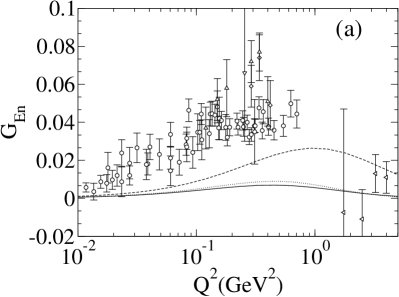
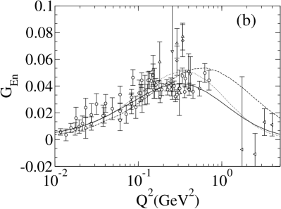
The point form result differs with what was already known from Ref. boffi . The only difference between both calculations being the wave functions employed, in our case simple 2 parametric symmetric wave functions, while in their case complicated wave functions obtained from the solution of their quark-quark hamiltonian. We noted the fact that in their wave functions there was a small admixture of mixed-symmetry s-state whose origin was the interaction between quarks. Thus, a phenomenological admixture was included in our wave function as described in section II. The results obtained with a 1% admixture are given in Fig. 6. The small admixture completely resolves the discrepancy in all the forms. The physical origin of such admixture must be sought in the quark-quark interaction.
4 transition in relativistic quark models
The electromagnetic transition is closely related to the presence of D-state components on both the and rest frame wave functions. A vast number of experiments have been dedicated to explore this transition and to extract model independent data for this reaction papanicolas ; cole .
The physical questions at hand are many, first, it is an appropriate place to study the effect of the so-called pion cloud satolee , which in the quark model picture would correspond to exploring the effects of including more fock space configurations in the wave function, e.g. RiskaLi ; ZouRiska .
Second, this transition is sensitive to the presence of components on the and wave function. The presence of such components is what is pursued when we talk about “Shape of Hadrons” (which is the title of this workshop). Several authors have discussed the issue of shape in the quark model framework in the recent years Miller ; Gross , although it seems at times that there is no clear meaning to the word “shape”. In the work of Miller Miller single quark spin dependent distribution functions are plotted as a proof of the existence of multiple shapes in the proton, in the work of Gross and Agbakpe Gross , on the contrary, it is stated explicitly that even the presence of D-state components on the proton would still render a symmetric charge distribution.
Formally the transition, can be characterized by the following set of form factors,
| (24) |
with,
| (25) |
where and are the nucleon and resonance masses respectively. The Sachs like magnetic dipole, electric quadrupole and Coulomb form factors are defined as in Ref. Scad ,
| (26) |
The relation between the three form factors and and the corresponding electric, magnetic and Coulomb form factors are Scad :
| (27) |
In instant and point form kinematics the relation between the different spin state matrix elements of the electromagnetic current and the form factors, , is finally:
| (28) |
Here the 4-momentum transfer is taken as , with , and
| (29) |
The and ratios for the transition are defined as:
| (30) |
Here .
4.1 Difficulties in the front form formulation
In the application of front form kinematics it has been conventional to adopt a reference frame in which . However, as explored in detail in Ref. dstate even if one works in such frame the equivalent to the angular condition is widely violated. That is, in front form there are four spin amplitudes which are linear combinations of only three form factors, , therefore they must be linearly dependent. This has also been studied by Cardarelli et al. simula ; simula2 for the same process, showing that in the single quark current approximation being used the angular condition cannot be fulfilled, implying that relativity is not correctly implemented. The reader is referred to those references for a deeper understanding of this point and we proceed to explore point and instant form calculations in our adopted single quark current approximation.
4.2 Results for instant and point form
Ratios of these form factors are commonly named and . There are definite pQCD predictions for them, at , . The non-relativistic quark model predictions at yield . Already 20 years ago, Ref. Weber studied the variation of in a relativistic quark model (front form) with symmetric rest frame wave functions. They found that would indeed become non-zero but extremely small, lower than .
Here their result is extended to the other forms of kinematics making use of the ground state wave functions found in the elastic case. Then, the simpler way to phenomenologically obtain structure in those ratios is by considering a D-state configuration in the rest frame wave function of both the and the as shown above. To explore all the possibilities the following wave functions for the and are considered:
with . In this exploratory study we are interested in the effect of state configurations in the wave functions. The following cases are considered: (,)= (0,0), (0.2,0), (0.2,0), (0,0.2) and (0,0.2).
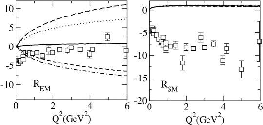
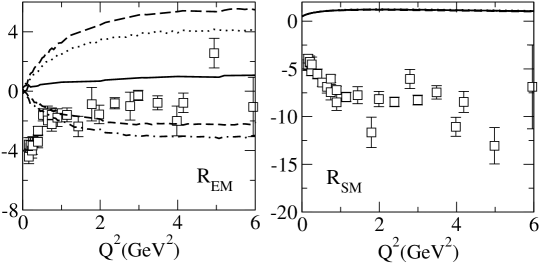
In figures 7 and 8 plots for the obtained results for instant and point form kinematics are given. The main features of the results are shared by both implementations of relativity, essentially when no state configuration is considered both the and ratios are small and quite different from the experimental data. The inclusion of a state configuration affects mainly the electric form factor and thus shows up abruptly in the ratio. The relative sign of the state configuration is relevant, it is found that a negative sign would be in line with the experimental data. This is so irrespective of whether it is the or the which contains the D-state configuration.
The situation is completely different for the ratio, there, the inclusion of such configuration does not give any seizable effect in either form.
Concerning the values at it becomes apparent from the figures that although they are not zero, due to the relativistic nature of the calculations, they are far from the few percent experimental values. Thus, the findings of Ref. Weber are confirmed also for instant and point form.
5 Summary and conclusion
Nucleons and low lying resonances in the energy domain of a few GeV are the perfect laboratory to study low energy QCD. There is a rich variety of resonances, meson-baryon states and maybe more exotic structures which coexist and which cannot yet be understood from the successful theory. The use of lattice QCD is a very promising one, and a great effort is being devoted to its implementation. At the same time, the effective field theory of the has also been presented (see Ref. pascalutsa ; gail ) and in its range of validity tends to agree with the experimental data. This effective theory, on the contrary, is only valid on a very narrow range.
Quark models, on the other hand, provide a organizational tool which allows to explore several relevant issues in strong physics. Here the way a quark model, which uses a simple spectral representation of the mass operator, is able to accommodate to a great extend the experimental form factors of the nucleon has been explained. Further refinements of the model in each of the forms could of course be pursued and a finer agreement with the data could most likely be achieved. An improvement which has been studied is the inclusion of anomalous magnetic moments for the constituent quarks, this of course would help resolve some of the discrepancies with the experimental data. On the other hand, up to now mostly three quark configurations have been considered when exploring the electromagnetic structure of hadrons and also in most studies of the baryon spectrum in quark models. The inclusion of higher components, both from a phenomenological point of view, and also from the solution of dynamical equations for the multiquark system needs to be further investigated. Small percentages of such higher configurations could play important roles in photoproduction and also in meson decays of resonances RiskaLi . This is to say, all the sensible configurations need to be exhausted before actually going into more complicated microscopic assumptions, such as the anomalous magnetic moments. In fact, the consideration of higher fock states is the natural step in the quark model in view of the recent dynamical studies which explain, to a certain extend, some resonances as molecular meson-baryon states. As an example, the dynamical model of Sato and Lee satolee , is able to reproduce the quotients and , being able to track down this success to their account of the so-called meson cloud effects.
Our study was aimed at exploring both the consequences of the different implementations of relativity and at the same time of the incorporation of non-S wave configurations on the wave functions.
With that in mind, the main learnings are:
-
•
The three forms of kinematics are able to describe the elastic form factors of the nucleon in a very reasonable way after fitting 2 parameters in the wave function plus the constituent quark mass. The fit is only constraint by the magnetic form factor of the proton. The higher tail of the form factors was however systematically underestimated by the point form calculation. The neutron electric form factor requires the inclussion of a small mixed-symmetry component on the rest frame wave function.
-
•
The only qualitative difference between the three forms appears in the presence of a node in the electric form factor of the proton. This node only appears, with the pointless quarks used here, in the front form calculation. The inclusion of mixed-symmetry components or state configurations would not change this picture. The node is in better agreement with the expected behavior after the recent JLAB measurements. The presence of nodes in front form form factors occurs also in the case of the rho and kaon form factors, see Ref. junheplb ; junheepja .
-
•
The issue of shape, phrased as importance of D-state components, has been addressed for the transition. There the results are both encouraging and not so. First, none of the forms is able to account for the structure present in the quotients, and , even when a D-state configuration is considered. Consideration of other fock state components, exchange currents and possibly resorting to anomalous magnetic moments for the constituent quarks could help resolve the problem. Front form calculations using single quark currents are of no interest for this transition as they are not fully relativistic.
References
- (1) P. L. Chung and F. Coester, Phys. Rev. D 44, 229 (1991).
- (2) F. Cardarelli, E. Pace, G. Salme and S. Simula, Phys. Lett. B 357, 267 (1995).
- (3) A. J. Buchmann, E. Hernandez and A. Faessler, Phys. Rev. C 55, 448 (1997).
- (4) S. Boffi, L. Y. Glozman, W. Klink, W. Plessas, M. Radici and R. F. Wagenbrunn, Eur. Phys. J. A 14, 17 (2002).
- (5) M. M. Giannini, these proceedings.
- (6) B. Julia-Diaz, D. O. Riska and F. Coester, Phys. Rev. C 69 (2004) 035212.
- (7) B. Julia-Diaz and D. O. Riska, Nucl. Phys. A 757 (2005) 441.
- (8) Q. B. Li and D. O. Riska, Nucl. Phys. A 766, 172 (2006); Q. B. Li and D. O. Riska, Phys. Rev. C 73, 035201 (2006).
- (9) P. A. M. Dirac, Rev. Mod. Phys., 49, 392 (1949).
- (10) B. D. Keister and W. N. Polyzou, Adv. Nucl. Phys. 20, 225 (1991).
- (11) F. Coester, Progress in Nuclear and Particle Physics 29, 1 (1992).
- (12) A. Amghar, B. Desplanques and L. Theussl, Phys. Lett. B 574, 201 (2003).
- (13) J. He, B. Julia-Diaz and Y. b. Dong, Phys. Lett. B 602, 212 (2004).
- (14) J. He, B. Julia-Diaz and Y. b. Dong, Eur. Phys. J. A 24, 411 (2005).
- (15) P. Mergell, U.-G. Meißner, D. Drechsel, Nucl. Phys. A 596, 367 (1996).
- (16) Jones et al., Phys Rev Lett 84, 1398 (2000); O. Gayou et al., Phys. Rev. Lett. 88, 092301 (2002).
- (17) J. Arrington, Phys. Rev. C69 022201 (2004).
- (18) K. Hagiwara et al., Phys. Rev. D 66, 010001 (2002).
- (19) F. Coester, private communication.
- (20) C. L. Smith, these proceedings.
- (21) C. Papanicolas, these proceedings.
- (22) T. Sato and T. S. H. Lee, Phys. Rev. C 54 (1996) 2660.
- (23) B. S. Zou and D. O. Riska, Phys. Rev. Lett. 95, 072001 (2005)
- (24) V. Pascalutsa, these proceedings.
- (25) T.A. Gail and T.R. Hemmert, these proceedings.
- (26) G. A. Miller and M. R. Frank, Phys. Rev. C 65, 065205 (2002)
- (27) F. Gross and P. Agbakpe, Phys. Rev. C 73, 015203 (2006).
- (28) H. F. Jones and M. D. Scadron, Ann. Phys. 81, 1 (1973).
- (29) F. Cardarelli, E. Pace, G. Salme and S. Simula, Nucl. Phys. A 623 (1997) 361C; F. Cardarelli, E. Pace, G. Salme and S. Simula, Phys. Lett. B 371 (1996) 7; E. Pace, G. Salme, F. Cardarelli and S. Simula, Nucl. Phys. A 666 (2000) 33.
- (30) J. Bienkowska, Z. Dziembowski and H. J. Weber, Phys. Rev. Lett. 59 (1987) 624 [Erratum-ibid. 59 (1987) 1790].
- (31) V. D. Burkert and T. S. H. Lee, Int. J. Mod. Phys. E 13 (2004) 1035.