Extended-soft-core baryon-baryon model
III. $S=-2$ hyperon-hyperon/nucleon interaction

Abstract

This paper presents the Extended-Soft-Core (ESC) potentials ESC04a-ESC04d for baryon-baryon channels with total strangeness $S=-2$. For these channels no experimental scattering data exist, and also the information from hypernuclei is very limited. The potential models for $S=-2$ are based on SU(3) extensions of potential models for the $S=0$ and $S=-1$ sectors, which are fitted to experimental data. Flavor SU(3)-symmetry is broken ’kinematically’ by the masses of the baryons and the mesons. Moreover, in ESC04a,b also the coupling constants are broken, albeit in a well defined way using the ${}^{3}P_{0}$ quark-antiquark pair creation model as a guidance. But, the fit to the $S=0$ and $S=-1$ sectors provides the necessary constraints to fix all free parameters. Therefore, the potentials for the $S=-2$ sectors do not contain additional free parameters, which situation is similar to the soft-core one-boson-exchange NSC97-models. Various properties of the potentials are illustrated by giving results for scattering lengths, bound states, phase-parameters, and total cross sections.

The features of $\Xi$ hypernuclei predicted by ESC04d are studied on the basis of the G-matrix approach.

I Introduction

In this paper the Extended-Soft-Core (ESC) potentials ESC04a-ESC04d, described in the companion nucleon-nucleon (N​N) Rij05 and the hyperon-nucleon (Y​N) paper RY05 , for baryon-baryon channels with total strangeness $S=-2$. These papers will be referred to as paper I and II respectively. In SR99 the Nijmegen soft-core one-boson-exchange (OBE) interactions NSC97a-f for baryon-baryon (BB) systems for $S=-2,-3,-4$ were presented.

For these channels hardly any experimental scattering information is available, and also the information from hypernuclei is very limited. There are data on double $\Lambda\Lambda$-hypernuclei, which recently became very much improved by the observation of the Nagara-event Tak01 . This event indicates that the $\Lambda\Lambda$-interaction is rather weak, in contrast to the estimates based on the older experimental observations Dan63 ; Pro66 .

In the virtual absense of experimental information, we assume that the potentials obey (broken) flavor SU(3) symmetry. As in I and II, the potentials are parametrized in terms of meson-baryon-baryon, and meson-pair-baryon-baryon couplings and gaussian form factors. This enables us to include in the interaction one-boson-exchange (OBE), two-pseudoscalar-exchange (TME), and meson-pair-exchange (MPE), without any new parameters. All parameters have been fixed by a simultaneous fit to the N​N and Y​N data, described in I and II. Each ${\it N\!N}\oplus{\it YN}$-model leads to a Y​Y-model in a well defined way. In II we have introduced four different models, called ESC04a-d, based on the options: SU(3)-symmetry breaking/ no-breaking of coupling constants, and pure pv/ pv-ps mixture for the pseudoscalar meson couplings. Then, SU(3)-symmetry allows us to define all coupling constants needed to describe the multi-strange interactions in the baryon-baryon channels occurring in $\{8\}\otimes\{8\}$. Most of the details on the SU(3) description are well known, and in particular for baryon-baryon scattering they can be found in papers I, II, and e.g. MRS89 ; RSY99 ; SR99 . So, here we restrict ourselves to a minimal exposition of these matters, necessary for the readability of this paper. Therefore, in Sec. II we first review for $S=-2$ the baryon-baryon multi-channel description, and present the SU(3)-symmetric interaction Lagrangian describing the interaction vertices between mesons and members of the $J^{P}={\textstyle(1/2)}^{+}$ baryon octet, and define their coupling constants. We then identify the various channels which occur in the $S=-2$ baryon-baryon systems. In appendix A the potentials on the isospin basis are given in terms of the SU(3)-irreps. In most cases, the interaction is a multi-channel interaction, characterized by transition potentials and thresholds. Details were given in SR99 ; RSY99 . For the details on the pair-interactions, we refer to II RY05 . In Sec. III we give a general treatment of the problem of flavor-exchange forces, which is very helpful to understand the proper treatment of exchange forces and the treatment of baryon-baryon channels with identical particles. In Sec. IV we describe briefly the treatment of the multi-channel threshods in the potentials. In Sec. V we present the results of the ESC04 potentials for all the sectors with total strangeness $S=-2$. We give the couplings and $F/(F+D)$-ratio’s for OBE-exchanges of ESC04a,d. Similarly, tables with the pair-couplings are shown in appendix B. We give the $S$-wave scattering lengths, discuss the possibility of bound states in these partial waves. Also, we give the S-matrix information for the elastic channels in terms of the Bryan-Klarsfeld-Sprung (BKS) phase parameters Bry81 ; Kla83 ; Spr85 , or in the Kabir-Kermode (KK) Kab87 format. Tables with the BKS-phase parameters are displayed in appendix C. Such information is very usefull for example for the construction of the $\Lambda$-, $\Sigma$-, and $\Xi$-nucleus potentials. We also give results for the total cross sections for all leading channels.

Important differences among the four versions ESC04a,b,c,d appear in their $\Xi N$ sectors. Table XXV in Ref. RY05 demonstrates that ESC04a,b (ESC04c,d) lead to repulsive (attractive) $\Xi$ potentials in nuclear matter. Especially, the $\Xi N$ interaction of ESC04d is attractive enough to produce various $\Xi$ hypernuclei. It is very interesting to study their features on the basis of the G-matrix approach. In Sec. VI, we represent the $\Xi N$ G-matrix interactions derived from ESC04d as density-dependent local potentials. In Sect. VII, structure calculations for $\Xi$ hypernuclei are performed with use of $\Xi$-nucleus folding potentials obtained from the G-matrix interactions. It is discussed how the features of ESC04d appear in the level structure of $\Xi$ hypernuclei. We conclude the paper with a summary and some final remarks in Sec. VIII.

II Channels, Potentials, and SU(3) Symmetry

II.1 Multi-channel Formalism

In this paper we consider the baryon-baryon reactions with $S=-2$

$$A_{1}(p_{a},s_{a})+B_{1}(p_{b},s_{b})\rightarrow A_{2}(p^{\prime}_{a},s^{\prime}_{a})+B_{2}(p^{\prime}_{b},s^{\prime}_{b})$$ (1)

Like in Ref.’s MRS89 ; RSY99 we will for the YN-channels also refer to $A_{1}$ and $A_{2}$ as particles 1 and 3, and to $B_{1}$ and $B_{2}$ as particles 2 and 4. For the kinematics and the definition of the amplitudes, we refer to paper I Rij05 of this series. Similar material can be found in MRS89 . Also, in paper I the derivation of the Lippmann-Schwinger equation in the context of the relativistic two-body equation is described.

On the physical particle basis, there are four charge channels:

$$q=+2:\ \ \Sigma^{+}\Sigma^{+}\rightarrow\Sigma^{+}\Sigma^{+},$$

$$q=+1:\ \ (\Xi^{0}p,\Sigma^{+}\Lambda,\Sigma^{0}\Sigma^{+})\rightarrow(\Xi^{0}p,\Sigma^{+}\Lambda,\Sigma^{0}\Sigma^{+}),$$

$$q=\ \ 0:\ \ (\Lambda\Lambda,\Xi^{0}n,\Xi^{-}p,\Sigma^{0}\Lambda,\Sigma^{0}\Sigma^{0},\Sigma^{-}\Sigma^{+})\rightarrow$$

$$(\Lambda\Lambda,\Xi^{0}n,\Xi^{-}p,\Sigma^{0}\Lambda,\Sigma^{0}\Sigma^{0},\Sigma^{-}\Sigma^{+}),$$

$$q=-1:\ \ (\Xi^{-}n,\Sigma^{-}\Lambda,\Sigma^{-}\Sigma^{0})\rightarrow(\Xi^{-}n,\Sigma^{-}\Lambda,\Sigma^{-}\Sigma^{0}),$$

$$q=-2:\ \ \Sigma^{-}\Sigma^{-}\rightarrow\Sigma^{-}\Sigma^{-}.$$ (2)

Like in MRS89 ; RSY99 , the potentials are calculated on the isospin basis. For $S=-2$ hyperon-nucleon systems there are three isospin channels:

$$I={\textstyle 0}:\ \ (\Lambda\Lambda,\Xi N,\Sigma\Sigma\rightarrow\Lambda\Lambda,\xi N,\Sigma\Sigma),$$

$$I={\textstyle 1}:\ \ (\Xi N,\Sigma\Lambda,\Sigma\Sigma\rightarrow\Xi N,\Sigma\Lambda,\Sigma\Sigma),$$

$$I={\textstyle 2}:\ \ \Sigma\Sigma\rightarrow\Sigma\Sigma.$$ (3)

Figure 1: Thresholds in YN- and YY-channels for $S=-2$.

For the kinematics of the reactions and the various thresholds, see RSY99 . In this work we do not solve the Lippmann-Schwinger equation, but the multi-channel Schrödinger equation in configuration space, completely analogous to MRS89 . The multi-channel Schrödinger equation for the configuration-space potential is derived from the Lippmann-Schwinger equation through the standard Fourier transform, and the equation for the radial wave function is found to be of the form MRS89

$$u^{\prime\prime}_{l,j}+(p_{i}^{2}\delta_{i,j}-A_{i,j})u_{l,j}-B_{i,j}u^{\prime}_{l,j}=0,$$ (4)

where $A_{i,j}$ contains the potential, nonlocal contributions, and the centrifugal barrier, while $B_{i,j}$ is only present when non-local contributions are included. The solution in the presence of open and closed channels is given, for example, in Ref. Nag73 . The inclusion of the Coulomb interaction in the configuration-space equation is well known and included in the evaluation of the scattering matrix.

Obviously, the potential on the particle basis for the $q=2$ and $q=-2$ channels are given by the $I={\textstyle 2}$ $\Sigma\Sigma$ potential on the isospin basis. For $q=0$ and $q=\pm 1$, the potentials are related to the potentials on the isospin basis by an isospin rotation. Using the indices $a,b,c,d$ for $\Lambda\Lambda,\Xi N,\Lambda\Sigma$, and $\Sigma\Sigma$ respectively, we have Mae95

$$V(q=0)=\left(\begin{array}[]{cccccc}V_{aa}&\sqrt{\textstyle\frac{1}{2}}V_{ba}&-\sqrt{\textstyle\frac{1}{2}}V_{ba}&0&-\sqrt{\textstyle\frac{1}{3}}V_{ad}&\sqrt{\textstyle\frac{1}{3}}V_{ad}\\[5.69054pt] \cdot&{\textstyle\frac{1}{2}}\left[V_{bb}(1)+V_{bb}(0)\right]&{\textstyle\frac{1}{2}}\left[V_{bb}(1)-V_{bb}(0)\right]&\sqrt{\textstyle\frac{1}{2}}V_{bc}&-\sqrt{\textstyle\frac{1}{6}}V_{bd}(0)&\sqrt{\textstyle\frac{1}{6}}V_{bd}(0)-{\textstyle\frac{1}{2}}V_{bd}(1)\\[5.69054pt] \cdot&\cdot&{\textstyle\frac{1}{2}}\left[V_{bb}(1)+V_{bb}(0)\right]&\sqrt{\textstyle\frac{1}{2}}V_{bc}&\sqrt{\textstyle\frac{1}{6}}V_{bd}(0)&-\sqrt{\textstyle\frac{1}{6}}V_{bd}(0)-{\textstyle\frac{1}{2}}V_{bd}(1)\\[5.69054pt] \cdot&\cdot&\cdot&V_{cc}&0&-\sqrt{\textstyle\frac{1}{2}}V_{cd}\\[5.69054pt] \cdot&\cdot&\cdot&\cdot&{\textstyle\frac{1}{3}}\left[2V_{dd}(2)+V_{dd}(0)\right]&{\textstyle\frac{1}{3}}\left[2V_{dd}(2)-V_{dd}(0)\right]\\[5.69054pt] \cdot&\cdot&\cdot&\cdot&\cdot&{\textstyle\frac{1}{6}}\left[V_{dd}(2)+3V_{dd}(1)+2V_{dd}(0)\right]\end{array}\right)\ ,$$ (5)

and for $q=+1$ we have

$$V(q=+1)=\left(\begin{array}[]{ccc}V_{bb}(1)&V_{bc}&-\sqrt{\textstyle\frac{1}{2}}V_{bd}\\[5.69054pt] V_{bc}&V_{cc}&-\sqrt{\textstyle\frac{1}{2}}V_{cd}\\[5.69054pt] -\sqrt{\textstyle\frac{1}{2}}V_{bd}(1)&-\sqrt{\textstyle\frac{1}{2}}V_{cd}&{\textstyle\frac{1}{2}}\left[V_{dd}(1)+V_{dd}(2)\right]\end{array}\right)\ ,$$ (6)

Here, when necessary an isospin label is added in parentheses.

The momentum space and configuration space potentials for the ESC04-model have been described in paper I Rij05 for baryon-baryon in general. Therefore, they apply also to hyperon-nucleon and we can refer for that part of the potential to paper I. Also in the ESC-model, the potentials are of such a form that they are exactly equivalent in both momentum space and configuration space. The treatment of the mass differences among the baryons are handled exactly similar as is done in MRS89 ; RSY99 . Also, exchange potentials related to strange meson exchanhe $K,K^{*}$ etc. , can be found in these references.

The baryon mass differences in the intermediate states for TME- and MPE- potentials has been neglected for YN-scattering. This, although possible in principle, becomes rather laborious and is not expected to change the characteristics of the baryon-baryon potentials.

II.2 Potentials and SU(3) Symmetry

We consider all possible baryon-baryon interaction channels, where the baryons are the members of the $J^{P}={\textstyle\frac{1}{2}}^{+}$ baryon octet

$$B=\left(\begin{array}[]{ccc}{\displaystyle\frac{\Sigma^{0}}{\sqrt{2}}+\frac{\Lambda}{\sqrt{6}}}&\Sigma^{+}&p\\[5.69054pt] \Sigma^{-}&{\displaystyle-\frac{\Sigma^{0}}{\sqrt{2}}+\frac{\Lambda}{\sqrt{6}}}&n\\[5.69054pt] -\Xi^{-}&\Xi^{0}&{\displaystyle-\frac{2\Lambda}{\sqrt{6}}}\end{array}\right).$$ (7)

The baryon masses, used in this paper, are given in Table 2. The meson nonets can be written as

$$P=P_{\rm sin}+P_{\rm oct},$$ (8)

where the singlet matrix $P_{\rm sin}$ has elements $\eta_{0}/\sqrt{3}$ on the diagonal, and the octet matrix $P_{\rm oct}$ is given by

$$P_{\rm oct}=\left(\begin{array}[]{ccc}{\displaystyle\frac{\pi^{0}}{\sqrt{2}}+\frac{\eta_{8}}{\sqrt{6}}}&\pi^{+}&K^{+}\\[5.69054pt] \pi^{-}&{\displaystyle-\frac{\pi^{0}}{\sqrt{2}}+\frac{\eta_{8}}{\sqrt{6}}}&K^{0}\\[5.69054pt] K^{-}&\overline{{K}^{0}}&{\displaystyle-\frac{2\eta_{8}}{\sqrt{6}}}\end{array}\right),$$ (9)

and where we took the pseudoscalar mesons with $J^{P}=0^{+}$ as a specific example. Introducing the following notation for the isodoublets,

$$N = \left(\begin{array}[]{c}p\\ n\end{array}\right),\ \ \ \Xi=\left(\begin{array}[]{c}\Xi^{0}\\ \Xi^{-}\end{array}\right),\ \ \ {\rm and}\$$ (14)

$$K = \left(\begin{array}[]{c}K^{+}\\ K^{0}\end{array}\right),\ \ \ K_{c}=\left(\begin{array}[]{c}\overline{K^{0}}\\ -K^{-}\end{array}\right),$$ (19)

the most general, SU(3) invariant, interaction Hamiltonian is then given by Swa63

$${\cal H}_{\rm pv}^{\rm oct} = g_{N\!N\pi}(\overline{N}\bm{\tau}N)\!\cdot\!\bm{\pi}-ig_{\Sigma\Sigma\pi}(\overline{\bm{\Sigma}}\!\times\!\bm{\Sigma})\!\cdot\!\bm{\pi}+g_{\Lambda\Sigma\pi}(\overline{\Lambda}\bm{\Sigma}+\overline{\bm{\Sigma}}\Lambda)\!\cdot\!\bm{\pi}+g_{\Xi\Xi\pi}(\overline{\Xi}\bm{\tau}\Xi)\!\cdot\!\bm{\pi}+$$ (20)

$$g_{\Lambda N\!K}\left[(\overline{N}K)\Lambda+\overline{\Lambda}(\overline{K}N)\right]+g_{\Xi\Lambda K}\left[(\overline{\Xi}K_{c})\Lambda+\overline{\Lambda}(\overline{K_{c}}\Xi)\right]+$$

$$g_{\Sigma N\!K}\left[\overline{\bm{\Sigma}}\!\cdot\!(\overline{K}\bm{\tau}N)+(\overline{N}\bm{\tau}K)\!\cdot\!\bm{\Sigma}\right]+g_{\Xi\Sigma K}\left[\overline{\bm{\Sigma}}\!\cdot\!(\overline{K_{c}}\bm{\tau}\Xi)+(\overline{\Xi}\bm{\tau}K_{c})\!\cdot\!\bm{\Sigma}\right]+$$

$$g_{N\!N\eta_{8}}(\overline{N}N)\eta_{8}+g_{\Lambda\Lambda\eta_{8}}(\overline{\Lambda}\Lambda)\eta_{8}+g_{\Sigma\Sigma\eta_{8}}(\overline{\bm{\Sigma}}\!\cdot\!\bm{\Sigma})\eta_{8}+g_{\Xi\Xi\eta_{8}}(\overline{\Xi}\Xi)\eta_{8}+$$

$$g_{N\!N\eta_{0}}(\overline{N}N)\eta_{0}+g_{\Lambda\Lambda\eta_{0}}(\overline{\Lambda}\Lambda)\eta_{0}+g_{\Sigma\Sigma\eta_{0}}(\overline{\bm{\Sigma}}\!\cdot\!\bm{\Sigma})\eta_{0}+g_{\Xi\Xi\eta_{0}}(\overline{\Xi}\Xi)\eta_{0},$$

where we again took the pseudoscalar mesons as an example, dropped the Lorentz character of the interaction vertices, and introduced the charged-pion mass to make the pseudovector coupling constant $f$ dimensionless. All coupling constants can be expressed in terms of only four parameters. The explicit expressions can be found in Ref. RSY99 . The $\Sigma$-hyperon is an isovector with phase chosen such Swa63 that

$$\bm{\Sigma}\!\cdot\!\bm{\pi}=\Sigma^{+}\pi^{-}+\Sigma^{0}\pi^{0}+\Sigma^{-}\pi^{+}.$$ (21)

This definition for $\Sigma^{+}$ differs from the standard Condon and Shortley phase convention Con35 by a minus sign. This means that, in working out the isospin multiplet for each coupling constant in Eq. (20), each $\Sigma^{+}$ entering or leaving an interaction vertex has to be assigned an extra minus sign. However, if the potential is first evaluated on the isospin basis and then, via an isospin rotation, transformed to the potential on the physical particle basis (see below), this extra minus sign will be automatically accounted for.

In appendix A, Table 17 and Table 18 we give the relation between the potentials on the isospin-basis, see (5)-(6), and the SU(3)-irreps.

Given the interaction Lagrangian (20) and a theoretical scheme for deriving the potential representing a particular Feynman diagram, it is now straightforward to derive the one-meson-exchange baryon-baryon potentials. We follow the Thompson approach Tho70 ; Rij91 ; Rij92 ; Rij96 and expressions for the potential in momentum space can be found in Ref. MRS89 . Since the nucleons have strangeness $S=0$, the hyperons $S=-1$, and the cascades $S=-2$, the possible baryon-baryon interaction channels can be classified according to their total strangeness, ranging from $S=0$ for $N\!N$ to $S=-4$ for $\Xi\Xi$. Apart from the wealth of accurate $N\!N$ scattering data for the total strangeness $S=0$ sector, there are only a few, and not very accurate, $Y\!N$ scattering data for the $S=-1$ sector, while there are no data at all for the $S<-1$ sectors. We therefore believe that at this stage it is not yet worthwhile to explicitly account for the small mass differences between the specific charge states of the baryons and mesons; i.e., we use average masses, isospin is a good quantum number, and the potentials are calculated on the isospin basis. The possible channels on the isospin basis are given in (3).

However, the Lippmann-Schwinger or Schrödinger equation is solved for the physical particle channels, and so scattering observables are calculated using the proper physical baryon masses. The possible channels on the physical particle basis can be classified according to the total charge $Q$; these are given in (2). The corresponding potentials are obtained from the potential on the isospin basis by making the appropriate isospin rotation. The matrix elements of the isospin rotation matrices are nothing else but the Clebsch-Gordan coefficients for the two baryon isospins making up the total isospin. (Note that this is the reason why the potential on the particle basis, obtained from applying an isospin rotation to the potential on the isospin basis, will have the correct sign for any coupling constant on a vertex which involves a $\Sigma^{+}$.)

In order to construct the potentials on the isospin basis, we need first the matrix elements of the various OBE exchanges between particular isospin states. Using the iso-multiplets (9) and the Hamiltonian (19) the isospin factors can be calculated. The results are given in Table 1, where we use the pseudoscalar mesons as a specific example. The entries contain the flavor-exchange operator $P_{f}$, which is $+1$ for a flavor symmetric and $-1$ for a flavor anti-symmetric two-baryon state. Since two-baryons states are totally anti-symmetric, one has $P_{f}=-P_{x}P_{\sigma}$. Therefore, the exchange operator $P_{f}$ has the value $P_{f}=+1$ for even-$L$ singlet and odd-$L$ triplet partial waves, and $P_{f}=-1$ for odd-$L$ singlet and even-$L$ triplet partial waves. In order to understand Table 1 fully, we have given in the following section Sec. III a general treatment of exchange forces. This treatment shows also how to deal with the case where the initial/final state involves identical particles and the final/inition state does not.

Second, we need to evaluate the TME and the MPE exchanges. The method we used for these is the same as for hyperon-nucleon, and is described in RY05 , Sec. IID.

III Exchange Forces

The proper treatment of the flavor-exchange forces is for the $S<-2$-channels more difficult than for the $S=0,1$-channels. The extra complication is the occurrence of coupling between channels with identical and non-identical particles. In order to understand the several $\sqrt{2}$-factors, see SR99 , we give here a systematic treatment of the flavor-exchange potentials. The method followed is using a multi-channel framework, which starts starts by ordering the two-particle states by assigning $A_{i}$ and $B_{i}$ for the channel labeled with the index $i$, like in eq. (1). The particles $A_{i}$ and $B_{i}$ have CM-momenta $p_{i}$ and $p_{i}^{\prime}$, spin components $s_{i}$ and $s_{i}^{\prime}$. The two-baryon states $|A_{i}B_{i}\rangle$ and $|B_{i}A_{i}\rangle$ are considered to be distinct, leading to distinct two-baryon channels. The ’direct’ and the ’exchange’ T-amplitudes are given by the T-matrix elements

$$\langle A_{j}B_{j}|T_{d}|A_{i}B_{i}\rangle,\ \ \langle B_{j}A_{j}|T_{e}|A_{i}B_{i}\rangle\ ,$$ (22)

and similarly for the direct and flavor-exchange potentials $V_{d}$ and $V_{e}$. It is obvious from rotation invariance that

$$\langle A_{j}B_{j}|T_{d}|A_{i}B_{i}\rangle = \langle B_{j}A_{j}|T_{d}|B_{i}A_{i}\rangle\ ,$$

$$\langle B_{j}A_{j}|T_{e}|A_{i}B_{i}\rangle = \langle A_{j}B_{j}|T_{e}|B_{i}A_{i}\rangle\ .$$ (23)

A similar definition (22) and relation (23) apply for the direct and flavor-exchange potentials $V_{d}$ and $V_{e}$.

We notice that there is here no exchange of momenta or spin-components. So, the momentum transfer for $V_{d}$ and $V_{e}$ is the same. Viewed from the coupled-channel scheme this is the normal situation.

The integral equations with two-baryon unitarity, e.g. the Thompson-, Lippmann-Schwinger-equation etc., reads for the $T_{d}$- and $T_{e}$-operator

$$\langle A_{j}B_{j}|T_{d}|A_{i}B_{i}\rangle = \langle A_{j}B_{j}|V_{d}|A_{i}B_{i}\rangle+\sum_{k}\left[\langle A_{j}B_{j}|V_{d}|A_{k}B_{k}\rangle\ G_{k}\ \langle A_{k}B_{k}|T_{d}|A_{i}B_{i}\rangle\right.$$ (24a)

$$\left.+\langle A_{j}B_{j}|V_{e}|A_{k}B_{k}\rangle\ G_{k}\ \langle A_{k}B_{k}|T_{e}|A_{i}B_{i}\rangle\ \right]\ ,$$

$$\langle B_{j}A_{j}|T_{e}|A_{i}B_{i}\rangle = \langle B_{j}A_{j}|V_{e}|A_{i}B_{i}\rangle+\sum_{k}\left[\langle B_{j}A_{j}|V_{d}|B_{k}A_{k}\rangle\ G_{k}\ \langle B_{k}A_{k}|T_{e}|A_{i}B_{i}\rangle\right.$$ (24b)

$$\left.+\langle B_{j}A_{j}|V_{e}|A_{k}B_{k}\rangle\ G_{k}\ \langle A_{k}B_{k}|T_{d}|A_{i}B_{i}\rangle\ \right]\ .$$

These coupled equations can be diagonalized by introducing the T- and V-operators

$$T^{\pm}=T_{d}\pm T_{e}\ ,\ \ V^{\pm}=V_{d}\pm V_{e}\ .$$ (25)

which satisfy separate integral equations

$$\langle A_{j}B_{j}|T^{\pm}|A_{i}B_{i}\rangle = \langle A_{j}B_{j}|V^{\pm}|A_{i}B_{i}\rangle+\sum_{k}\langle A_{j}B_{j}|V^{\pm}|A_{k}B_{k}\rangle\ G_{k}\ \langle A_{k}B_{k}|T^{\pm}|A_{i}B_{i}\rangle\ .$$ (26)

Notice that on the basis of states with definite flavor symmetry

$$|A_{i}B_{i}\rangle_{\pm}=\frac{1}{\sqrt{2}}\left[|A_{i}B_{i}\rangle\pm|B_{i}A_{i}\rangle\right]\ ,$$ (27)

the $T^{\pm}$ and $V^{\pm}$ matrix elements are also given by

$$T^{\pm}_{ij}=_{\pm}\!\!\langle A_{i}B_{i}|T|A_{j}B_{j}\rangle_{\pm}\ ,\ \ V^{\pm}_{ij}=_{\pm}\!\!\langle A_{i}B_{i}|V|A_{j}B_{j}\rangle_{\pm}\ .$$ (28)

III.1 Identical Particles

Sofar, we considered the general case where $A_{i}\neq B_{i}$ for all channels. In the case that $A_{i}=B_{i}$ for some $i$, one has $\langle B_{i}A_{i}|V_{e}|A_{i}B_{i}\rangle=0$, because there is no distinct physical state corresponding to the ’flavor exchange-state’. For example for a flavor single channel like $pp$ one deduces from (24b) that then also $T_{e}=0$, and one has in this case the integral equation

$$\langle A_{j}B_{j}|T_{d}|A_{i}B_{i}\rangle=\langle A_{j}B_{j}|V_{d}|A_{i}B_{i}\rangle+$$

$$\sum_{k}\langle A_{j}B_{j}|V_{d}|A_{k}B_{k}\rangle\ G_{k}\ \langle A_{k}B_{k}|T_{d}|A_{i}B_{i}\rangle\ ,$$ (29)

where the labels $i$ and $j$ now denote e.g. the spin-components.

III.2 Coupled $\Lambda\Lambda$ and $\Xi N$ system

This multi-channel system represents the case where there is mixture of channels with identical and with non-identical particles. The three states we distinguish are $|\Lambda\Lambda\rangle,|\Xi N\rangle$, and $|N\Xi\rangle$. Choosing the same ordering, the potential written as a $3x3$-matrix reads

$$V=\left(\begin{array}[]{ccc}(\Lambda\Lambda|V|\Lambda\Lambda)&(\Lambda\Lambda|V|\Xi N)&(\Lambda\Lambda|V|N\Xi\\ (\Xi N|V|\Lambda\Lambda)&(\Xi N|V|\Xi N)&(\Xi N|V|N\Xi\\ (N\Xi|V|\Lambda\Lambda)&(N\Xi|V|\Xi N)&(N\Xi|V|N\Xi\end{array}\right)\ .$$ (30)

With a similar notation for the T-matrix, the Lippmann-Schwinger equation can be written compactly as a $3x3$-matrix equation:

$$T=V+V\ G\ T\ ,\ {\rm with}\ G_{ij}=G_{i}\ \delta_{ij}\ .$$ (31)

Next, we make a transformation to states, which are either symmetric or anti-symmetric for particle interchange. Then, according to the discussion above, we can separate them in the Lippmann-Schwinger equation. This is achieved by the transformation

$$\left(\begin{array}[]{c}\Lambda\Lambda\\ \Xi N\\ N\Xi\end{array}\right)\Rightarrow\left(\begin{array}[]{c}\Lambda\Lambda\\ (\Xi N+N\Xi)/\sqrt{2}\\ (\Xi N-N\Xi)/\sqrt{2}\end{array}\right)=\left(\begin{array}[]{ccc}1&0&0\\ 0&1/\sqrt{2}&1/\sqrt{2}\\ 0&1/\sqrt{2}&-1/\sqrt{2}\end{array}\right)\left(\begin{array}[]{c}\Lambda\Lambda\\ \Xi N\\ N\Xi\end{array}\right)\ .$$ (32)

one gets in the transformed basis for the potential

$$UVU^{-1}=\left(\begin{array}[]{cll}V_{\Lambda\Lambda;\Lambda\Lambda}&(V_{\Lambda\Lambda;\Xi N}+V_{\Lambda\Lambda;N\Xi})/\sqrt{2}&(V_{\Lambda\Lambda;\Xi N}-V_{\Lambda\Lambda;N\Xi})/\sqrt{2}\\ (V_{\Xi N;\Lambda\Lambda}+V_{N\Xi;\Lambda\Lambda})/\sqrt{2}&(V_{\Xi N;\Xi N}+V_{\Xi N;N\Xi})&\hskip 40.68723pt0\\ (V_{\Xi N;\Lambda\Lambda}-V_{N\Xi;\Lambda\Lambda})/\sqrt{2}&\hskip 40.68723pt0&(V_{\Xi N;\Xi N}-V_{\Xi N;N\Xi})\\ \end{array}\right)\ ,$$ (33)

and of course, a similar form is obtained for the T-matrix on the transformed basis. Now, obviously we have that $V_{\Lambda\Lambda;\Xi N}=V_{\Lambda\Lambda;N\Xi}$ and $V_{\Xi N;\Lambda\Lambda}=V_{N\Xi;\Lambda\Lambda}$. Therefore, one sees that the even and odd states under particle exchange are decoupled in (33). Also $V_{\Xi N;\Lambda\Lambda}+V_{N\Xi;\Lambda\Lambda}=\sqrt{2}V_{\Xi N;\Lambda\Lambda}$, etc. showing the appearance of the $\sqrt{2}$-factors, mentioned before. Indeed, they appear in a systematic way using the multi-channel framework.

III.3 The K-exchange Potentials

Consider for example the $(\Lambda\Lambda,\Xi N)$-system, having $I=0$. Mesons with strangeness, $K(495)$, $K^{*}(892)$, $\kappa(900)$, $K_{1}(1270)$, are obviously the only ones that can give transition potentials, i.e. $V_{\Lambda\Lambda;\Xi N}\neq 0$ and $V_{\Xi N;\Lambda\Lambda}\neq 0$. The $\Xi N(I=0)$-states anti-symmetric and symmetric in flavor are respectively:

$$P_{f}=-1:\ \frac{1}{\sqrt{2}}\left[|\Xi N(I=0)\rangle-|N\Xi(I=0)\rangle\right]\ ,$$ (34a)

$$P_{f}=+1:\ \frac{1}{\sqrt{2}}\left[|\Xi N(I=0)\rangle+|N\Xi(I=0)\rangle\right]\ .$$ (34b)

Analyzing the ${}^{1}S_{0}$-state one has because of the anti-symmetry of the two-fermion state w.r.t. the exchange of all quantum labels, $P_{f}=-P_{\sigma}P_{x}=+1$, where $P_{f}$ denotes the flavor-symmetry. Taking here the $K(495)$ as a generic example, and using (19) and (20), one finds that

$$\langle\Xi^{0}n|V(K)|\Lambda\Lambda\rangle=+g_{K\Lambda N}g_{K\Xi N},\ \ \langle\Xi^{-}p|V(K)|\Lambda\Lambda\rangle=-g_{K\Lambda N}g_{K\Xi N}\ .$$ (35)

Taking here the $K(495)$ as a generic example, Then, since $|\Xi N(I=0)\rangle=\left[|\Xi^{0}n\rangle-|\Xi^{-}p\rangle\right]/\sqrt{2}$, one obtains for the ’direct’ potential the coupling

$$V_{\Xi N;\Lambda\Lambda}=\langle\Xi N(I=0)\rangle|V_{d}(K)|\Lambda\Lambda\rangle\Leftarrow\sqrt{2}g_{K\Lambda N}g_{K\Xi N}\ .$$ (36)

The same result is found for the ’exchange’ potential $V_{N\Xi;\Lambda\Lambda}$. Therefore

$$\frac{1}{\sqrt{2}}\left(V_{\Xi N;\Lambda\Lambda}+V_{N\Xi;\Lambda\Lambda}\right)=\langle\Xi N(I=0)|V(K)|\Lambda\Lambda\rangle\Leftarrow 2g_{K\Lambda N}g_{K\Xi N}\ ,$$ (37)

which has indeed the $(1+P_{f})$-factor given in Table 1, and is identical to Table IV in SR99 , for $(\Lambda\Lambda|K|\Xi N)$.

For $\langle\Xi N|K|\Sigma\Lambda\rangle$ the entry for $I=1$ consists of two parts. These correspond to $V_{d}\propto g_{\Lambda NK}g_{\Xi\Sigma K}$ and $V_{e}\propto g_{\Sigma NK}g_{\Xi\Lambda K}$ respectively, i.e. the direct and exchange contributions involve different couplings. Therefore, they are not added together.

III.4 The $\eta$- and $\pi$-exchange Potentials

Next, we discuss briefly the computation of the entries for $\eta$- and $\pi$-exchange in Table 1. First, the entries with — indicate that the corresponding physical state does not exist. Next we give further specific remarks and calculations:

1. For $\eta,\eta^{\prime}$-exchange one has that $V_{e}=0$. The matrix elements for the $\Lambda\Lambda$- and $\Xi N$-state are easily seen to be correct. For the $\Sigma\Sigma$-states one has $P_{f}=1$ for $I_{\Sigma\Sigma}=0,2$, and $P_{f}=-1$ for $I_{\Sigma\Sigma}=1$. This explains the $\Sigma\Sigma$ matrix element.

2. For $\langle\Xi N|\pi|\Xi N\rangle$ the computation is identical to that for NN, in particular $pn$.

3. For $\langle\Sigma\Sigma|\pi|\Sigma\Sigma\rangle$ consider the $I=0,I_{3}=0$ and $I=1,I_{3}=0$ matrix elements. In these cases one has $V_{e}=0$ as one can easily check. Then, using the cartesian base, we have for $\langle\Sigma_{i}\Sigma_{m}|\pi|\Sigma_{j}\Sigma_{n}\rangle\Rightarrow-g_{\Sigma\Sigma\pi}^{2}\sum_{p=1}^{3}\epsilon_{jip}\epsilon_{nmp}=-g_{\Sigma\Sigma\pi}^{2}(\delta_{jn}\delta_{im}-\delta_{jm}\delta_{in})$. Employing the states $|I=0,I_{3}=0\rangle\sim-\sum_{i,m=1}^{3}\delta_{im}|\Sigma_{i}\Sigma_{m}\rangle/\sqrt{3}$ and $|I=1,I_{3}=0\rangle\sim-i\sum_{i,m=1}^{3}\epsilon_{im3}|\Sigma_{i}\Sigma_{m}\rangle/\sqrt{2}$, one obtains the results in Table 1.

With the ingredients given above one can easily check the other entries in Table 1.

Table 1: Isospin factors for the various meson exchanges in the different total strangeness and isospin channels. $P_{f}$ is the flavor-exchange operator. The $I=2$ case only contributes to $S=-2$ $\Sigma\Sigma$ scattering, where the isospin factors can collectively be given by $(\Sigma\Sigma|\eta,\eta^{\prime},\pi|\Sigma\Sigma)={\textstyle\frac{1}{2}}(1+P_{f})$, and so they are not separately displayed in the table. Non-exixisting channels are marked by a long-dash.

$S=-2$	$I=0$	$I=1$
$(\Lambda\Lambda|\eta,\eta^{\prime}|\Lambda\Lambda)$	${\textstyle\frac{1}{2}}(1+P_{f})$	—
$(\Xi N|\eta,\eta^{\prime}|\Xi N)$	${\textstyle\frac{1}{2}}(1+P_{f})$	1
$(\Sigma\Sigma|\eta,\eta^{\prime}|\Sigma\Sigma)$	${\textstyle\frac{1}{2}}(1+P_{f})$	${\textstyle\frac{1}{2}}(1-P_{f})$
$(\Sigma\Lambda|\eta,\eta^{\prime}|\Sigma\Lambda)$	—	1
$(\Xi N|\pi|\Xi N)$	$-3$	1
$(\Sigma\Sigma|\pi|\Sigma\Sigma)$	$-(1+P_{f})$	$-{\textstyle\frac{1}{2}}(1-P_{f})$
$(\Lambda\Lambda|\pi|\Sigma\Sigma)$	$-{\textstyle\frac{1}{2}}\sqrt{3}(1+P_{f})$	—
$(\Sigma\Lambda|\pi|\Lambda\Sigma)$	—	$P_{f}$
$(\Sigma\Sigma|\pi|\Sigma\Lambda)$	—	$(1-P_{f})$
$(\Lambda\Lambda|K|\Xi N)$	$1+P_{f}$	—
$(\Sigma\Sigma|K|\Xi N)$	$\sqrt{3}(1+P_{f})$	$\sqrt{2}(1-P_{f})$
$(\Xi N|K|\Sigma\Lambda)$	—	$\sqrt{2};-P_{f}\sqrt{2}$

IV Multi-channel Thresholds and Potentials

IV.1 Thresholds

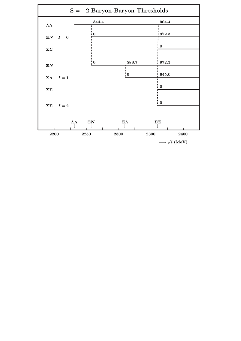
Clearly, the $S=-2$ two-baryon channels represent a number of separate coupled-channel systems, separated by the charge, see (2). A further subdivision is according to the total isospin. The different thresholds have been discussed in detail in SR99 , and we show them here in Fig. 1 for the purpose of general orientation. Their presence turns the Lippmann-Schwinger and Schrödinger equation into a coupled-channel matrix equation, where the different channels open up at different energies. In general one has a combination of ’open’ and ’closed’ channels. For a discussion of the solution of such a mixed system, we refer to Swa71 .

IV.2 Threshold- and Meson-mass corrections in Potentials

As discussed in SR99 , the one-meson-exchange Feynman-graph consists actually of two three-dimensional time-ordered graphs. The energy denominator from these two diagrams reads

$$D(\omega)=\frac{1}{2\omega}\left[\frac{1}{E_{2}+E_{3}-W+\omega}+\frac{1}{E_{1}+E_{4}-W+\omega}\right],$$ (38)

where, $W=\sqrt{s}$ is the total energy and $\omega^{2}={\bf k}^{2}+m^{2}$, with $m$ the meson mass and ${\bf k}={\bf p}^{\prime}-{\bf p}$ the momentum transfer. From (38) it is clear that the potential is energy dependent. We use the static approximation $E_{i}\rightarrow M_{i}$ and $W\rightarrow M^{0}_{1}+M^{0}_{2}$, where the superscript 0 refers to the masses of the lowest threshold of the particular coupled-channel system q, see (2). They are in general not equal to the masses $M_{1}$ and $M_{2}$ occurring in the time-ordered diagrams. For example, the potential for the $\Sigma\Sigma$ contribution in the coupled-channel $\Lambda\Lambda$ system has $M_{1}=M_{2}=M_{\Sigma}$, but $M^{0}_{1}=M^{0}_{2}=M_{\Lambda}$. Denoting $a\equiv E_{2}+E_{3}-W\approx M_{2}+M_{3}-M^{0}_{1}-M^{0}_{2}>0$, and similarly for $E_{1}+E_{4}-W$, we have for the ’propagators’ Rij92 for $0<a<m$

$$\frac{1}{\omega(\omega+a)}=\frac{2}{\pi}\int_{0}^{\infty}\frac{ad\lambda}{(a^{2}+\lambda^{2})(\omega^{2}+\lambda^{2})}\ .$$ (39)

This integral representation makes it possible to deal with it numerically rather exactly. However, we think that such a sophistication is unnecessary at present nor for a description of the $S=-1$ scattering data, nor for $S=-2$. where there are virtually no data at all. Therefore, we handle with this approximately as follows:

1. Elastic potentials: In this case we use (39), and in (38) one has $E_{1}=E_{3}\approx M_{i}$ and $E_{2}=E_{4}\approx M^{\prime}_{i}$, for the elastic channel, label $i$. Here $a\approx M_{i}+M^{\prime}_{i}-M_{1}^{0}-M_{2}^{0}$. Then,

$$D_{i}(\omega) = \frac{1}{\omega^{2}}+\Delta_{i}(\omega,a),\ \ \Delta_{i}(\omega,a)=\frac{2}{\pi}\int_{0}^{\infty}\frac{d\lambda}{a^{2}+\lambda^{2}}\cdot$$ (40)

$$\times\left[\frac{1}{\omega^{2}}-\frac{1}{\omega^{2}+\lambda^{2}}\right]\ ,$$

for $0<a<m$. Because of this condition we apply this not to the pseudoscalars, but to the vector-, scalar-, and axial-mesons. For example, in the case of the $\Lambda\Lambda$-scattering, the $\Sigma\Sigma$-channel potential is reduced by this effect. Since the $\Sigma\Sigma$-channel is rather far away from the others, we in practice apply (40) only for that channel. In this case $a>0$ and the $\theta(-a)$-term in $D_{i}(\omega)$ vanishes.

2. Inelastic potentials: In this case, like in SR99 and all other papers on the Nijmegen potentials, we use the approximation of Swa62 , using the fact that $M_{1}^{0}+M_{2}^{0}$ is mostly rather close to the average of the initial and final-sate baryon masses. Then, the propagator can be written as

$$D(\omega)\rightarrow\frac{1}{\omega^{2}-{\textstyle\frac{1}{4}}(M_{3}-M_{4}+M_{2}-M_{1})^{2}},$$ (41)

which amounts to introducing an effective meson mass $\overline{m}$

$$m^{2}\rightarrow\overline{m}^{2}=m^{2}-{\textstyle\frac{1}{4}}(M_{3}-M_{4}+M_{2}-M_{1})^{2}.$$ (42)

For more details of this effect on the exchanged meson masses, we refer to SR99 .

Table 2: Baryon masses in MeV/$c^{2}$.

Baryon		Mass
Nucleon	$p$	938.2796
	$n$	939.5731
Hyperon	$\Lambda$	1115.60
	$\Sigma^{+}$	1189.37
	$\Sigma^{0}$	1192.46
	$\Sigma^{-}$	1197.436
Cascade	$\Xi^{0}$	1314.90
	$\Xi^{-}$	1321.32

The used baryon masses are about the same as in SR99 , and are given in Table 2. The used meson masses are the same as in paper II RY05 , as well as the cut-off mases.

V Results

The main purpose of this paper is to present the properties of the four ESC04 potentials for the $S=-2$ sector. We will show the detailed results for ESC04a and ESC04d, which are sufficient to represent the possible kind of results. Model ESC04a is representative for the inclusion of SU(3)-breaking of the couplings, and ESC04d for the case of SU(3)-symmetric couplings. The free parameters in each model are fitted to the $N\!N$ and $Y\!N$ scattering data for the $S=0$ and $S=-1$ sectors, respectively. Given the expressions for the coupling constants in terms of the octet and singlet parameters and their values for the six different models as presented in Ref. RSY99 , it is straightforward to evaluate all possible baryon-baryon-meson coupling constants needed for the $S\leq-2$ potentials. A complete set of coupling constants for models ESC04a and ESC04d is given in Tables 3 and 4, respectively.

In Fig’s 2 and Fig. 3 we display the OBE potentials for the individual pseudoscalar, vector, scalar, and axial mesons in the case of model ESC04d.

Table 3: Coupling constants for model ESC04a, divided by $\sqrt{4\pi}$. $M$ refers to the meson. The coupling constants are listed in the order pseudoscalar, vector ($g$ and $f$), scalar, and diffractive.

Type	$M$	$N\!N\!M$	$\Sigma\Sigma M$	$\Sigma\Lambda M$	$\Xi\Xi M$		$M$	$\Lambda N\!M$	$\Lambda\Xi M$	$\Sigma N\!M$	$\Sigma\Xi M$
$f$	$\pi$	0.2631	0.2456	0.1620	–0.0175		$K$	–0.2179	0.0977	0.0130	–0.1951
$g$	$\rho$	0.7800	1.5600	0.0000	0.7800		$K^{*}$	–1.0022	1.0022	–0.5786	–0.5786
$f$		3.4711	1.9177	2.9009	–1.5535			–2.3080	0.1560	1.1524	–2.5750
$g$	$a_{1}$	2.5426	1.1922	2.2477	–1.3505		$K_{1}$	–1.1597	–0.0492	0.7263	–1.3675
$g$	$a_{0}$	0.9251	1.5562	0.1698	0.6311		$\kappa$	–1.0506	0.9261	–0.4628	–0.6785
$g$	$a_{2}$	0.00000	0.00000	0.00000	0.00000		$K^{**}$	0.00000	0.00000	0.00000	0.00000
Type	$M$	$N\!N\!M$	$\Lambda\Lambda M$	$\Sigma\Sigma M$	$\Xi\Xi M$		$M$	$N\!N\!M$	$\Lambda\Lambda M$	$\Sigma\Sigma M$	$\Xi\Xi M$
$f$	$\eta$	0.1933	–0.0203	0.2153	–0.1161		$\eta^{\prime}$	0.1191	0.1421	0.1167	0.1525
$g$	$\omega$	3.0135	2.2104	2.2104	1.4073		$\phi$	–0.3849	–0.9611	–0.9611	–1.5372
$f$		0.4467	–1.4028	2.0461	–1.5278			–0.0502	–1.3771	1.0973	–1.4667
$g$	$f_{1}$	1.0190	0.7973	1.2595	0.8067		$f^{\prime}_{1}$	1.0352	–0.2915	2.4744	–0.2352
$g$	$\varepsilon$	3.4635	2.5842	2.7926	1.8090		$f_{0}$	–0.8162	–1.3699	–1.2387	–1.8580
$g$	$P$	1.9651	1.9651	1.9651	1.9651		$f_{2}$	0.0000	0.0000	0.0000	0.0000

Table 4: Coupling constants for model ESC04d, divided by $\sqrt{4\pi}$. $M$ refers to the meson. The coupling constants are listed in the order pseudoscalar, vector ($g$ and $f$), scalar, and diffractive.

Type	$M$	$N\!N\!M$	$\Sigma\Sigma M$	$\Sigma\Lambda M$	$\Xi\Xi M$		$M$	$\Lambda N\!M$	$\Lambda\Xi M$	$\Sigma N\!M$	$\Sigma\Xi M$
$f$	$\pi$	0.2599	0.2592	0.1505	–0.0008		$K$	–0.2997	0.1492	0.0008	–0.2599
$g$	$\rho$	0.7038	1.4076	0.0000	0.7038		$K^{*}$	–1.2190	1.2190	–0.7038	–0.7038
$f$		3.2909	2.8332	2.1642	–0.4577			–3.5357	1.3715	0.4577	–3.2909
$g$	$a_{1}$	2.4310	1.1398	2.1490	–1.2912		$K_{1}$	–2.0616	–0.0874	1.2912	–2.4310
$g$	$a_{0}$	1.0303	1.7331	0.1891	0.7028		$\kappa$	–1.5955	1.4064	–0.7028	–1.0303
$g$	$a_{2}$	0.00000	0.00000	0.00000	0.00000		$K^{**}$	0.00000	0.00000	0.00000	0.00000
Type	$M$	$N\!N\!M$	$\Lambda\Lambda M$	$\Sigma\Sigma M$	$\Xi\Xi M$		$M$	$N\!N\!M$	$\Lambda\Lambda M$	$\Sigma\Sigma M$	$\Xi\Xi M$
$f$	$\eta$	0.2125	–0.0634	0.2137	–0.2007		$\eta^{\prime}$	0.1188	0.2359	0.1183	0.2942
$g$	$\omega$	3.0366	2.2944	2.2944	1.5523		$\phi$	–0.7935	–1.7606	–1.7606	–2.7277
$f$		0.0052	–2.1472	0.4878	–2.9822			1.7248	–1.0803	2.3537	–2.1684
$g$	$f_{1}$	1.7228	2.5283	0.8489	2.4941		$f^{\prime}_{1}$	0.6363	–1.2614	2.6950	–1.1810
$g$	$\varepsilon$	3.5434	3.2267	3.3017	2.9475		$f_{0}$	0.7172	–0.8465	–0.4759	–2.2249
$g$	$P$	2.3532	2.3532	2.3532	2.3532		$f_{2}$	0.0000	0.0000	0.0000	0.0000

In the following we will present the model predictions for scattering lengths, bound states, and cross sections.

Figure 2: ESC04d: OBE contributions to the $(^{1}S_{0},I=0)$ potentials for the PS, V, S, and A meson nonets.

Figure 3: ESC04d: OBE contributions to the $(^{3}S_{1},I=0)$ potentials for the PS, V, S, and A meson nonets.

Figure 4: ESC04d $(^{1}S_{0},I=0)$ $\Lambda\Lambda$-phases. The dashed curve n.c. is the case with no coupling to the $\Xi N,\Sigma\Sigma$ channels.

Figure 5: ESC04d $I=0$ $\Xi N$-phases.

Figure 6: ESC04d $I=1$ $\Xi N$-phases. The dashed curve n.c. is the case with no coupling to the $\Sigma\Lambda,\Sigma\Sigma$ channels.

Figure 7: ESC04d $I=1$ $\Sigma\Lambda$-phases.

V.1 Effective-range parameters

For ESC04a the $I=0$ low-energy parameters are

$$a_{\Lambda\Lambda}(^{1}S_{0}) = -3.804\ [fm]\ ,\ \ r_{\Lambda\Lambda}(^{1}S_{0})=2.420\ [fm]\ .$$

$$a_{\Xi N}(^{3}S_{1}) = -1.672\ [fm]\ ,\ \ r_{\Xi N}(^{3}S_{1})=2.704\ [fm]\ .$$

For ESC04d the $I=0$ low-energy parameters are

$$a_{\Lambda\Lambda}(^{1}S_{0}) = -1.555\ [fm]\ ,\ \ r_{\Lambda\Lambda}(^{1}S_{0})=3.617[fm]\ .$$

$$a_{\Xi N}(^{3}S_{1}) = +122.5\ [fm]\ ,\ \ r_{\Xi N}(^{3}S_{1})=2.083\ [fm]\ .$$

Table 5: $I=0$: Inverse-scattering-length and effective-range matrices at the $\Xi N$ threshold. The order of the states (1-2) reads $\Lambda\Lambda(^{1}S_{0}),\Xi N(^{1}S_{0})$. The dimension of the matrix elements are in [fm]${}^{-1}(A^{-1}$ and [fm]$(R)$.

	ESC04a		ESC04d
	$A^{-1}$	$R$	$A^{-1}$	$R$
11	–0.929	4.114	–0.584	3.484
12	0.667	–0.318	0.840	–1.666
22	1.108	1.494	0.470	1.626

Table 6: $I=1$: Inverse-scattering-length and effective-range matrices at the $\Xi N$ threshold. The order of the states (1-2) reads $\Lambda\Lambda(^{1}S_{0}),\Xi N(^{1}S_{0})$. The dimension of the matrix elements are in [fm]${}^{-1}(A^{-1}$ and [fm]$(R)$.

	ESC04a		ESC04d
	$A^{-1}$	$R$	$A^{-1}$	$R$
11	0.281	2.752	–0.121	4.878
12	–4.067	–1.643	–0.977	1.851
22	–1.603	2.888	–0.380	2.028

Table 7: $I=1$: Inverse-scattering-length and effective-range matrices at the $\Xi N$ threshold. The order of the states (1-2) reads $\Lambda\Lambda(^{3}S_{1}),\Lambda\Lambda(^{3}D_{1}),\Xi N(^{3}S_{1})$. The dimension of the matrix elements are in [fm]${}^{-1-l-l^{\prime}}(A^{-1}$ and [fm]${}^{1-l-l^{\prime}}(R)$.

	ESC04a		ESC04d
	$A^{-1}$	$R$	$A^{-1}$	$R$
11	1.484	4.896	0.021	139.289
12	–0.856	–11.999	0.015	–517.222
13	1.621	–8.293	–0.046	–160.711
22	270.392	–422.973	–0.009	5933.937
23	0.348	36.874	0.045	1471.645
33	–2.156	15.785	–0.274	382.035

For $I=1$ we have for ESC04a:

$$a_{\Xi N}(^{1}S_{0}) = 0.491\ [fm]\ ,\ \ r_{\Xi N}(^{1}S_{0})=-0.421\ [fm]\ .$$

For $I=1$ we have for ESC04d:

$$a_{\Xi N}(^{1}S_{0}) = 0.144\ [fm]\ ,\ \ r_{\Xi N}(^{1}S_{0})=4.670\ [fm]\ .$$

For the $S=-2$ sector the results are given in Table 5-7. The $\Lambda\Lambda(^{1}S_{0})$ scattering lengths are found to be larger than in the NSC97 models, indicating an attractive $\Lambda\Lambda$ interaction, which is strongest in ESC04a.

The old experimental information seemed to indicate a separation energy of $\Delta B_{\Lambda\Lambda}=4-5$ MeV, corresponding to a rather strong attractive $\Lambda\Lambda$ interaction. As a matter of fact, an estimate for the $\Lambda\Lambda$ ${}^{1}S_{0}$ scattering length, based on such a value for $\Delta B_{\Lambda\Lambda}$, gives $a_{\Lambda\Lambda}(^{1}S_{0})\approx-2.0$ fm Tan65 ; Bod65 . However, in recent years the experimental information and interpretation of the ground state levels of ${}_{\Lambda\Lambda}^{\,\ 6}$He, ${}_{\Lambda\Lambda}^{\;10}$Be, and ${}_{\Lambda\Lambda}^{\;13}$B Dal89 , has been changed drastically. This because of the Nagara-event Tak01 , identified uniquely as ${}_{\Lambda\Lambda}^{\,\ 6}$He Tak01 , which established that the $\Lambda\Lambda$-interaction is weaker ($\Delta B_{\Lambda\Lambda}\approx 1$ MeV).

In NSC97 RSY99 we could only increase the attraction in the $\Lambda\Lambda$ channel by modifying the scalar-exchange potential. If the scalar mesons are viewed as being mainly $q\bar{q}$ states, one finds that the (attractive) scalar-exchange part of the interaction in the various channels satisfies

$$|V_{\Lambda\Lambda}|<|V_{\Lambda N}|<|V_{N\!N}|,$$ (43)

suggesting indeed a rather weak $\Lambda\Lambda$-potential. The NSC97 fits to the $Y\!N$ scattering data RSY99 give values for the scalar-meson mixing angle which seem to point to almost ideal mixing for the scalars as $q\bar{q}$ states, and we found that an increased attraction in the $\Lambda\Lambda$ channel would give rise to (experimentally unobserved) deeply bound states in the $\Lambda N$ channel. On the other hand, in the ESC04 models we have in principle more possibilities because of the presence of meson-pair poteials. As one sees from the values of the $a_{\Lambda\Lambda}(^{1}S_{0})$ in the ESC04 models of this paper we can produce the apparently required attraction in the $\Lambda\Lambda$ interaction without giving rise to $\Lambda N$ bound states (see below). Notice that also in ESC04 we have scalar mixings close to ideal ones, akin to NSC97. The large values for the triplet effective range $r_{t}$ in $\Xi N$ is a simple reflection of the fact that the ${}^{3}S_{1}$ phase shift at small laboratory momenta is very small and only very slowly increases in magnitude.

V.2 Bound states in $\bm{S}$ waves

A discussion of the possible bound-states, using the SU(3) content of the different $S=0,-1,-2$ channels is given in RSY99 . As in RSY99 , for a general orientation, we list in Table 8 all the irreps to which the various baryon-baryon channels belong. In contrast to the NSC97 models, we find almost no bound states in the ESC04a-d models. An exception is model ESC04d, where there occurs a $\Xi N$ bound state in the ${}^{3}S_{1}$-${}^{3}D_{1}$ coupled partial wave. From Table 8 one sees that this is a $\{8_{a}\}$-state, which is a little bit surprising. This because the OBE-potential one expects to be rather repulsive in the irrep $\{8_{a}\}$, see MRS89 . However, in the ESC04 models this situation is changed because of the contribution of the axial-vector-mesons, and the meson pairs, cfrm. Fig. 8. The differences between ESC04a and ESC04d for this channel are in the OBE and MPE, and accidentally there is a bound-state in ESC04d but not in ESC04a.

Figure 8: ESC04d: $\Xi N(^{3}S_{1},I=0)$-potentials. The solid-, dashed-, and short-dashed-line are respectively the total-, central-, and spin-spin-potentials.

Table 8: SU(3) content of the different interaction channels. $S$ is the total strangeness and $I$ is the isospin. The upper half refers to the space-spin symmetric states ${}^{3}S_{1}$, ${}^{1}P_{1}$, ${}^{3}D$, …, while the lower half refers to the space-spin antisymmetric states ${}^{1}S_{0}$, ${}^{3}P$, ${}^{1}D_{2}$, …

Space-spin symmetric
$S$	$I$	Channels	SU(3)-irreps
0	0	$N\!N$	$\{10^{*}\}$
–1	1/2	$\Lambda N$, $\Sigma N$	$\{10^{*}\}$, $\{8\}_{a}$
	3/2	$\Sigma N$	$\{10\}$
–2	0	$\Xi N$	$\{8\}_{a}$
	1	$\Xi N$, $\Sigma\Sigma$	$\{10\}$, $\{10^{*}\}$, $\{8\}_{a}$
		$\Sigma\Lambda$	$\{10\}$, $\{10^{*}\}$
Space-spin antisymmetric
$S$	$I$	Channels	SU(3)-irreps
0	1	$N\!N$	$\{27\}$
–1	1/2	$\Lambda N$, $\Sigma N$	$\{27\}$, $\{8\}_{s}$
	3/2	$\Sigma N$	$\{27\}$
–2	0	$\Lambda\Lambda$, $\Xi N$, $\Sigma\Sigma$	$\{27\}$, $\{8\}_{s}$, $\{1\}$
	1	$\Xi N$, $\Sigma\Lambda$	$\{27\}$, $\{8\}_{s}$
	2	$\Sigma\Sigma$	$\{27\}$

From Table 8 one notices that this $\Xi N$-channel is not a mixture of different SU(3)-irreps, and so form this point of view simple. The same thing is for $S=-2$ only true for the $\Sigma\Sigma(^{1}S_{0},I=2)$-channel. The other $S=-2$ channels are are mixtures of at least two irreps, which makes an analysis of the presence or absence of bound states more difficult, as pointed out in RSY99 . For the models ESC04a-d we did not find any $S$-wave bound states in these ’mixed’ channels.

V.3 Partial Wave Phase Parameters

For the BB-channels below the inelastic threshold we use for the parametrization of the amplitudes the standard nuclear-bar phase shifts SYM57 . The information on the elastic amplitudes above thresholds is most conveniently given using the BKS-phases Bry81 ; Kla83 ; Spr85 . For uncoupled partial waves, the elastic BB $S$-matrix element is parametrized as

$$S=\eta e^{2i\delta}\ ,\ \ \eta=\cos(2\rho)\ .$$ (44)

For coupled partial waves the elastic BB-amplitudes are $2\times 2$-matrices. The BKS $S$-matrix parametrization, which is of the type-S variety, is given by

$$S=e^{i\delta}e^{i\epsilon}N\ e^{i\epsilon}e^{i\delta}\ ,$$ (45)

where

$$\delta=\left(\begin{array}[]{cc}\delta_{\alpha}&0\\ 0&\delta_{\beta}\end{array}\right)\ ,\ \ \epsilon=\left(\begin{array}[]{cc}0&\epsilon\\ \epsilon&0\end{array}\right)\ ,$$ (46)

and $N$ is a real, symmetric matrix parametrize as

$$N=\left(\begin{array}[]{cc}\eta_{11}&\eta_{12}\\ \eta_{12}&\eta_{22}\end{array}\right)\ .$$ (47)

From the various parametrizations of the $N$-matrix, we choose the Kabir-Kermode parametrization Kab87 to represent the $N$-matrix in the figures. Then, the $N$-matrix is given by the inelasticity parameters $(\alpha,\beta,\varphi)$, called $\rho$-parameters, as follows

$$N=\left(\begin{array}[]{cc}\cos(2\alpha)&\sin(\varphi+\xi)\\ \sin(\varphi+\xi)&\cos(2\beta)\end{array}\right)\ ,$$ (48)

where

$$\alpha=\pm\frac{1}{2}\cos^{-1}(\eta_{11})\ \ ,\ \ \beta=\pm\frac{1}{2}\cos^{-1}(\eta_{22})\ ,$$

$$\varphi=\sin^{-1}(\eta_{12})-sgn(\eta_{12})\sin^{-1}Q\$$

$$\xi=sgn(\eta_{12})\sin^{-1}Q\ .$$ (49)

Here

$$Q^{2}=1-|\eta_{11}+\eta_{22}|+\eta_{11}\eta_{22}\ .$$ (50)

In Fig’s 4-7 the BKS-phases and coupling parameters $(\alpha,\beta,\varphi)$ for ESC04d are shown. In Fig 4 and Fig. 6 we also show the ${}^{1}S_{0}$-phases (n.c.) for the case with no coupling to the other two-particle channels. For $\Lambda\Lambda$ the n.c.-curve shows that the potential is repulsive, which is mainly due to the $\{1\}$-irrep. The attraction comes in particular from the coupling to the $\Xi N$-channel.

In the Tables 21-30, we give for the models ESC04a,d the inelasticity parameters $\rho$ and $\eta_{11},\eta_{12},\eta_{22}$, which enable the reader to construct the $N$-matrix most directly.

V.4 Total cross sections

We next present the predictions for the total cross section for several channels. We suppose always that the beam as well as the target are unpolarized. Therefore, we incuded the statistical factors, which are $1/4$ for the spin-singlet and $3/4$ for the spin-triplet case.

In Fig. 9 we present the elastic $\Lambda\Lambda$ and the inelastic $\Lambda\Lambda\rightarrow\Xi N$ total cross sections. Being dominantly S-wave, there is in principle has a (sharp) cusp at the $\Xi N$-threshold, i.e. $p_{\Lambda}=344.4$ MeV/$c^{2}$.

In Fig. 10 we present the $\Xi N$ and $\Sigma\Lambda$ elastic and the, $\Xi N\rightarrow\Lambda\Lambda$ and $\Sigma\Lambda\rightarrow\Xi N$ inelastic total cross sections.

For those cases where both baryons are charged, we do not include the purely Coulomb contribution to the total cross section, nor do we include the Coulomb interference to the nuclear amplitude. The cross section is calculated by summing the contributions from partial waves with orbital angular momentum up to and including $L=2$. We find this to be sufficient for all the $S\neq 0$ sectors; inclusion of any higher partial waves has no significant effect. Inclusion of higher partial waves will shift the total cross section to slightly higher values without changing the overall shape. Of course, their inclusion would be necessary if a detailed comparison with real experimental data were to be made.

Figure 9: ESC04d $I=0$ $\sigma_{T}(\Lambda\Lambda$) and $\sigma_{T}(\Xi N)$.

Figure 10: ESC04d $I=1$ $\sigma_{T}(\Xi N)$ and $\sigma_{T}(\Sigma\Lambda)$.

In Table 9 we show the $\Lambda\Lambda\rightarrow\Lambda\Lambda,\Xi N$ total X-sections as a function of the laboratory momentum $p_{\Lambda}$. In Table 10 we show the $\Xi N\rightarrow\Xi N,\Lambda\Lambda$ total X-sections as a function of the laboratory momentum $p_{\Xi}$. In Table 11 we show the $\Xi N\rightarrow\Xi N,\Sigma\Lambda$ total X-sections as a function of the laboratory momentum $p_{\Xi}$. In Table 12 we show the $I=1,L=0$ $\Sigma\Lambda\rightarrow\Sigma\Lambda,\Xi N,\Sigma\Sigma$ total X-sections as a function of the laboratory momentum $p_{\Sigma}$.

Table 9: $(I=0,L=0)$ Total X-sections $\Lambda\Lambda\rightarrow\Lambda\Lambda,\Xi N$ in [mb] as a function of the laboratory momentum $p_{\Lambda}$ in [MeV]

	ESC04a		ESC04d
$p_{\Lambda}$	$\Lambda\Lambda$	$\Xi N$	$\Lambda\Lambda$	$\Xi N$
10	447.92	—	75.59	—
50	326.93	—	66.71	—
100	171.59	—	47.39	—
200	50.31	—	18.51	—
300	17.72	—	7.45	—
350	11.30	0.72	6.87	2.56
400	5.90	1.42	2.74	4.37
500	1.50	1.19	0.95	3.44
600	0.22	0.89	1.04	2.57
700	0.07	0.67	1.48	1.99
800	0.34	0.51	1.87	1.60
900	0.73	0.39	2.13	1.33
1000	1.10	0.30	2.34	1.02

Table 10: $(I=0,L=0)$ Total X-sections $\Xi N\rightarrow\Xi N,\Lambda\Lambda$ in [mb] as a function of the laboratory momentum $p_{\Xi}$ in [MeV]

	ESC04a		ESC04d
$p_{\Xi}$	$\Xi N$	$\Lambda\Lambda$	$\Xi N$	$\Lambda\Lambda$
10	184.19	278.99	708.56	187x103
50	35.67	259.62	129.80	8496.85
100	16.84	212.47	57.73	2073.20
200	7.25	118.22	22.73	461.11
300	4.08	63.66	12.12	168.70
400	2.58	36.51	7.48	73.17
500	1.76	22.90	5.07	34.51
600	1.26	15.83	3.68	17.52
700	0.94	12.02	2.81	9.98
800	0.72	9.90	2.23	6.83
900	0.56	8.71	1.83	5.76
1000	0.44	8.06	1.48	5.53

Table 11: $(I=1,L=0)$ Total X-sections $\Xi N\rightarrow\Xi N,\Sigma\Lambda$ in [mb] as a function of the laboratory momentum $p_{\Xi}$ in [MeV]

	ESC04a		ESC04d
$p_{\Xi}$	$\Xi N$	$\Sigma\Lambda$	$\Xi N$	$\Sigma\Lambda$
10	297.54	—-	15.68	—-
50	278.46	—-	15.00	—-
100	233.23	—-	13.11	—-
200	142.04	—-	7.99	—-
300	87.03	—-	3.91	—-
400	57.54	—-	1.77	—-
500	41.08	—-	0.85	—-
600	28.31	2.22	0.98	3.27
700	20.64	3.63	2.55	3.21
800	16.73	3.38	3.19	2.45
900	14.10	3.27	3.62	2.20
950	15.26	1.59	11.88	3.69
1000	12.60	2.34	8.45	1.85

Table 12: $(I=1,L=0)$ Total X-sections $\Sigma\Lambda\rightarrow\Sigma\Lambda,\Xi N,\Sigma\Sigma$ in [mb] as a function of the laboratory momentum $p_{\Sigma}$ in [MeV]

	ESC04a			ESC04d
$p_{\Sigma}$	$\Sigma\Lambda$	$\Xi N$	$\Sigma\Sigma$	$\Sigma\Lambda$	$\Xi N$	$\Sigma\Sigma$
10	671.52	31.36	—-	1406.84	46.55	—-
50	127.24	29.40	—-	223.90	36.19	—-
100	58.38	26.51	—-	84.93	24.49	—-
200	24.24	20.73	—-	26.67	10.17	—-
300	13.63	16.18	—-	12.38	4.87	—-
400	8.92	13.06	—-	6.96	4.26	—-
500	6.56	10.74	—-	4.50	5.50	—-
600	5.86	12.39	—-	4.41	7.13	—-
650	3.70	13.53	2.04	3.85	7.92	0.81
700	3.60	11.00	2.31	2.50	8.35	0.46
800	3.40	9.48	1.82	1.85	9.24	0.17
900	3.24	8.59	1.67	1.56	9.76	0.26
1000	3.03	7.92	1.67	1.36	9.94	0.54

VI $\Xi N$ G-matrix interaction

As demonstrated in our previous works RSY99  RY05 , the G-matrix theory is very convenient to explore the features of YN and YY interaction models in nuclear medium. Table XXV in Ref.RY05 demonstrates the basic features of the $\Xi N$ G-matrix interactions derived from ESC04a,b,c,d. It is important, here, that some versions (ESC04c,d) lead to the attractive $\Xi$-nucleus potentials $U_{\Xi}$, predicting the existence of $\Xi$ hypernuclei owing to their strong ${}^{13}S_{1}$ attractions. (A two-body spin- and isospin-state is represented by ${}^{(2I+1)(2S+1)}L_{J}$.) In the present, the most reliable information for $U_{\Xi}$ is considered to be given by the BNL-E885 experiment E885 , in which they measured the missing mass spectra for the ¹²C$(K^{-},K^{+})$X reaction. Reasonable agreement between this data and theory is realized by assuming a $\Xi$-nucleus potential $U_{\Xi}(\rho)=-V_{0}f(r)$ with well depth $V_{0}\sim 14$ MeV within the Wood-Saxon prescription, named here as WS14.

Table 13: $\Xi$ single particle energies $U_{\Xi}$ and conversion widths $\Gamma_{\Xi}$ at normal density calculated with ESC04d and NHC-D. $S$-state contributions in spin- and isospin- states and total $P$-state contributions are also given. All entries are in MeV.

	${}^{11}S_{0}$	${}^{13}S_{1}$	${}^{31}S_{0}$	${}^{33}S_{1}$	$P$	$U_{\Xi}$	$\Gamma_{\Xi}$
ESC04d($\alpha=0$)	6.4	$-$19.6	6.4	$-$5.0	$-$6.9	$-$18.7	11.4
ESC04d($\alpha=.18$)	6.3	$-$18.4	7.2	$-$1.7	$-$5.6	$-$12.1	12.7
NHC-D	$-$2.6	0.7	$-$2.3	$-$0.4	$-$16.8	$-$21.4	1.1

Among the four versions of ESC04 models, only ESC04d seems to be compatible with WS14. In Table 13, we recapitulate the G-matrix result for ESC04d, where the partial-wave contributions to $U_{\Xi}$ are shown. The most important is here that the attractive values of $U_{\Xi}$ for ESC04d are due to the strong attractions in the ${}^{13}S_{1}$ state. The difference between the two versions of ESC04d specified by values of $\alpha$ is as follows: In Ref.RY05 , the medium-induced repulsion was taken into account by changing masses of vector mesons in medium with use of the parameter $\alpha_{V}$. Then, it was shown that this effect plays important roles to reproduce nuclear saturation and $\Lambda$ well depth. It is quite reasonable to take this effect into account also in $\Xi$ hypernuclear systems: A criterion for $\alpha_{V}$ is the value of 0.18 used successfully in $S=0$ and $-1$ cases. However, we should not stick to this value, because there is no definite information for $\Xi$ hypernuclei experimentally in the present. A reasonable way for us is to consider it as a changeable parameter to study features of $\Xi$ states. Hereafter, the parameter $\alpha_{V}$ is denoted as $\alpha$ simply.

In this work, the imaginary parts of G-matrices in ${}^{11}S_{1}$ and ${}^{13}P_{J}$ states are taken into account together with their real parts. The imaginary parts are due to the energy-conserving transitions from $\Xi N$ to $\Lambda\Lambda$ channels in nuclear medium. For simplicity, we evaluate them in perturbation, the real parts being the same as those in Ref.RY05 . Then, the conversion width $\Gamma_{\Xi}$ is obtained from the imaginary part of $U_{\Xi}$ by multiplying $-2$. The calculated values of $\Gamma_{\Xi}$ are also given in Table 13.

It should be stressed here that the features of the $\Xi N$ interaction in ESC04d are distinctly different from those in OBE models. Among the Nijmegen OBE models, only the Nijmegen hard-core model D (NHC-D) NRS77 is known to give the attractive value of $U_{\Xi}$ adequately owing to its peculiar modeling, where octet scalar mesons are not taken into account. For comparison, the result for NHC-D is also given in Table 13, where the hard-core radii $r_{c}$ are taken so as to reproduce $\Xi$-nucleus interactions compatibly to WS14: The value of $r_{c}$ in ${}^{11}S_{0}$ state is taken as 0.53 fm, and those in the other channels as 0.47 fm. The former value is chosen so that the $\Lambda\Lambda$ interaction in this channel is consistent with the data of ${}^{\ 6}_{\Lambda\Lambda}$He. The features of NHC-D are found to be quite different from those of ESC04d($\alpha$): The attractive value of $U_{\Xi}$ in this case is dominated by the $P$-state contribution, and the calculated value of $\Gamma_{\Xi}$ is far smaller than those of ESC04d($\alpha$).

Table 14: Parameters $c_{ij}$ in Eq.51 for ESC04d($\alpha$).

Real Parts
		$I=0$			$I=1$
	$c_{1j}^{(+)}$	$-$896.7	$-$181.5	$-$1865.	11.10	34.07	$-$50.69
${}^{1}E$	$c_{2j}^{(+)}$	1632.	356.4	3236.	61.19	$-$95.18	115.8
	$c_{3j}^{(+)}$	$-$573.1	$-$153.3	$-$1457.	3.896	83.62	$-$63.83
	$c_{1j}^{(+)}$	$-$641.7	18.39	86.11	$-$35.84	33.02	.8333
${}^{3}E$	$c_{2j}^{(+)}$	582.3	$-$39.56	$-$144.4	20.39	$-$96.59	$-$5.139
	$c_{3j}^{(+)}$	$-$197.9	64.61	63.89	8.864	95.87	4.944
	$c_{1j}^{(-)}$	312.4	$-$13.64	26.39	$-$171.4	23.08	29.17
${}^{1}O$	$c_{2j}^{(-)}$	75.00	13.86	$-$19.58	124.9	$-$79.25	$-$87.50
	$c_{3j}^{(-)}$	20.00	15.24	3.611	$-$21.81	111.7	55.55
	$c_{1j}^{(-)}$	$-$331.4	4.944	580.6	$-$108.2	39.69	43.06
${}^{3}O$	$c_{2j}^{(-)}$	39.75	$-$47.36	$-$1326.	24.25	$-$120.1	$-$113.6
	$c_{3j}^{(-)}$	81.25	98.96	760.4	3.636	127.0	69.78

Imaginary Parts ($I=0$)
	$c_{1j}^{(+)}$	$-$292.0	$-$916.9	569.4
${}^{1}E$	$c_{2j}^{(+)}$	32.47	2096.	$-$1621.
	$c_{3j}^{(+)}$	19.74	$-$1152.	1059.
	$c_{1j}^{(-)}$	$-$10.55	1.619	$-$523.2
${}^{3}O$	$c_{2j}^{(-)}$	3.295	3.817	1178.
	$c_{3j}^{(-)}$	$-$1.242	$-$8.286	$-$655.1

Now, our concern is to investigate how appear the features of ESC04d in level structures of various $\Xi$ hypernuclei. For such an aim, it is convenient to represent $\Xi N$ G-matrix interactions in nuclear matter as density-dependent local potentials Yam94 . Because sophisticated constructions of coordinate-space G-matrices are not necessary under our poor knowledge on $\Xi$ hypernuclei, we adopt here the following simple method: Our G-matrix interaction in each isospin- and spin-state is given in a two-range Gaussian form

$$G^{(\pm)}_{IS}(r,k_{F})=(C_{1}^{(\pm)}+C_{2}^{(\pm)}k_{F}+C_{3}^{(\pm)}k_{F}^{2})\cdot$$

$$\times\exp{(-(r/0.8)^{2})}+C_{0}\,\exp{(-(r/1.6)^{2})}\ ,$$

$$C_{i}^{(\pm)}=\sum^{3}_{j=1}c_{ij}^{(\pm)}\,\alpha^{j-1}\qquad{\rm for}\ \ i=1,2,3$$ (51)

where the density-dependence is represented as a function of a Fermi momentum $k_{F}$. The suffices $(+)$ and $(-)$ specify even and odd states, respectively. Parameters $C_{i}^{(\pm)}$ are determined as follows: First, the outer-range part is fixed so as to simulate the tail part of the bare interaction. The adopted values of $C_{0}$ are $-3.73$ MeV (${}^{11}E$, ${}^{11}O$), $-5.29$ MeV (${}^{13}E$, ${}^{13}O$), $-3.34$ MeV (${}^{31}E$, ${}^{31}O$) and $-4.93$ MeV (${}^{33}E$, ${}^{33}O$). Next, the strengths of the inner-range parts are determined so as to reproduce the partial-wave contributions to $U_{\Xi}$ in $(ISL)$ states. The $k_{F}$ dependence is determined by using the results for the three values of $k_{F}=$ 1.35, 1.00, 0.80 fm^-1. For convenience, the coefficients $C_{i}^{(\pm)}(i=1,2,3)$ in each $(IS)$ state are given as a quadratic function of $\alpha$, which represents all together the G-matrix interactions for ESC04d with various values of $\alpha$. The parameters $c_{ij}^{(\pm)}$ for ESC04d($\alpha$) are listed in Table 14.

VII Applications to $\Xi$ hypernuclei

VII.1 A folding-model

$\Xi$-nucleus potentials in finite systems are constructed by folding our G-matrix interactions $G^{(\pm)}_{IS}(r,k_{F})$ into nuclear-core density distributions with a local density approximation (LDA). Taking into account the Lane term, our potential $U_{\Xi}$ is given by

$$U_{\Xi}({\bf r},{\bf r^{\prime}})=U_{0}({\bf r},{\bf r^{\prime}})+U_{1}({\bf r},{\bf r^{\prime}})\,{\bf t_{\Xi}}\cdot{\bf T_{c}}/A_{c}\ ,$$

$$U_{i}({\bf r},{\bf r^{\prime}})=\delta({\bf r}-{\bf r^{\prime}})\int d{\bf r^{\prime\prime}}\rho({\bf r^{\prime\prime}})\,\left[V_{i}^{(+)}(|{\bf r}-{\bf r^{\prime\prime}}|;k_{F})+\right.$$

$$\left.V_{i}^{(-)}(|{\bf r}-{\bf r^{\prime\prime}}|;k_{F})\right]/2+\rho({\bf r},{\bf r^{\prime}})\left[V_{i}^{(+)}(|{\bf r}-{\bf r^{\prime}}|;k_{F})-\right.$$

$$\left.V_{i}^{(-)}(|{\bf r}-{\bf r^{\prime}}|;k_{F})\right]/2\ ,\quad(i=0,1)\ ,$$ (52)

with $k_{F}({\bf r},{\bf r^{\prime}})=[3\pi^{2}/2\cdot(\rho({\bf r})+\rho({\bf r^{\prime}}))/2]^{1/3}$. The terms $V_{i}^{(\pm)}$ are expressed by combinations of $G^{(\pm)}_{IS}$ as

$$V_{0}^{(\pm)} = (3G^{(\pm)}_{10}+3G^{(\pm)}_{01}+G^{(\pm)}_{00}+9G^{(\pm)}_{11})/16,$$

$$V_{1}^{(\pm)} = (G^{(\pm)}_{10}-3G^{(\pm)}_{01}-G^{(\pm)}_{00}+3G^{(\pm)}_{11})/4,$$ (53)

where ${\bf T_{c}}$ and ${\bf t_{\Xi}}$ are isospins of a core nucleus and a $\Xi$ particle, respectively, and $A_{c}$ is a mass number of a core nucleus. Spin-dependent parts of $\Xi-$nucleus potentials are not considered in our present studies.

Here, we study only the diagonal part of the ${\bf t_{\Xi}}\cdot{\bf T_{c}}$ term, though the $\Xi^{-}-\Xi^{0}$ mixing effect induced by its non-diagonal part is important to specify some feature of an underlying $\Xi N$ interaction Lanskoy . Nuclear cores are assumed to be spherically symmetric, and density $\rho(r)$ and mixed density $\rho(r,r^{\prime})$ are constructed from nuclear wave functions given by the density-dependent Hartree-Fock (DDHF) calculations with the Skyrme-III interaction Skyrme3 . It should be noted here that the $\Xi N$ space-exchange parts are treated accurately in our treatment. In the present modeling, the difference between $\Xi^{-}-$ and $\Xi^{0}-$nucleus potentials comes from the Lane term, when the Coulomb interactions are switched off.

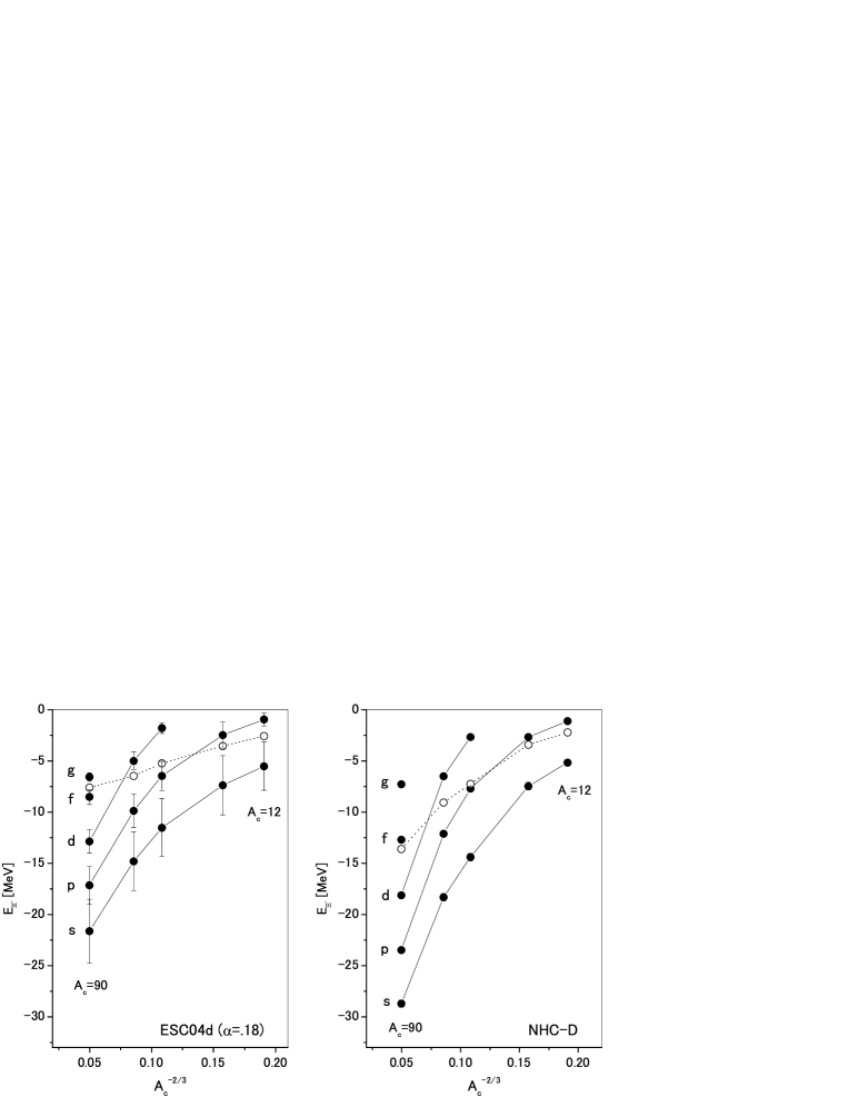
First, let us show the results for simple systems composed of spin- and isospin-saturated nuclear cores attached by a $\Xi^{-}$ particle; ¹²C+$\Xi^{-}$, ¹⁶O+$\Xi^{-}$, ²⁸Si+$\Xi^{-}$, ⁴⁰Ca+$\Xi^{-}$, ⁹⁰Zr+$\Xi^{-}$, where Coulomb interactions between $\Xi^{-}$ and nuclear cores are taken into account. In these systems, there is no contribution from the Lane term except the case of ⁹⁰Zr core. In the left and right sides of Fig.1, full circles connected by solid lines show the single particle (s.p.) energies of $\Xi^{-}$-bound states calculated with G-matrix interactions derived from ESC04d($\alpha=.18$) and NHC-D, respectively, as a function of ${A_{c}}^{-2/3}$. The “error bars” in the figure present the calculated values of conversion widths $\Gamma_{\Xi}$, though they are not visible in the case of NHC-D. The conversion widths for ESC04d are found to be remarkably larger than those for NHC-D, because the $\Xi N$-$\Lambda\Lambda$ coupling interaction in the ${}^{11}S_{0}$ state in the former is far stronger than that in the latter. This feature can be seen in our result for the double-$\Lambda$ nucleus ${}^{\ 6}_{\Lambda\Lambda}$He: As shown in Table XXIV of Ref.RY05 , ESC04d brings about a large value of the $\Xi N$ admixture probability $P_{\Xi N}$ in ${}^{\ 6}_{\Lambda\Lambda}$He due to the strong $\Lambda\Lambda$-$\Xi N$ coupling interaction. If this coupling is switched off in this case, no reasonable $\Lambda\Lambda$ bound state can be obtained.

The open circles connected by dotted lines give the $s$-state energies of $\Xi^{0}$. It is noted that the Coulomb contributions to $\Xi^{-}$ binding energies are substantial in large mass-number systems. Hereafter, when a $\Xi$ particle can be bound without an assist from a $\Xi$-nucleus Coulomb interaction, we call it a $\Xi$-nuclear bound state. In the figure, $p$-states in ¹²C and ¹⁶O, $d$-states in ²⁸Si and ⁴⁰Ca, $f$- and $g$-states in ⁹⁰Zr are so-called Coulomb-assisted states. Namely, these $\Xi$ states become unbound when Coulomb interactions are switched off, though their wave functions deviate substantially from pure Coulomb ones. On the other hand, the $f$-state in ⁹⁰Zr for NHC-D is a $\Xi$-nuclear bound state.

ESC04d and NHC-D give rise to similar values of $\Xi^{-}$ s.p. energies in the ¹²C core. In the large mass-number region, however, the $\Xi^{-}$ s.p. energies for NHC-D are far deeper than those for ESC04d($\alpha=.18$), the reason why is because the $\Xi$-nucleus interaction for NHC-D is dominated by contributions from odd-state attractions. There is no space-exchange term in OBE parts, because strangeness $-2$ cannot be carried by a single boson. This is the reason why the odd-state interactions in NHC-D are so attractive.

In the case of ⁹⁰Zr+$\Xi^{-}$, the contributions from the Lane terms are +1.3 and +0.2 MeV for ESC04d($\alpha=.18$) and NHC-D, respectively. It should be noted that the lane term in ESC04d is far stronger than that in NHC-D.

Next, we study more realistic $\Xi$ hypernuclei produced by $p(K^{-},K^{+})\Xi^{-}$ reactions on available nuclear targets. In Table 15, our results for ESC04d($\alpha=.18$) and ESC04d($\alpha=0$) are listed in some cases of $N=Z$ targets (⁶Li, ¹²C, ¹⁶O, ²⁸Si, ⁴⁰Ca) and $N>Z$ targets (¹¹B, ²⁷Al, ⁴⁸Ca), $Z$ and $N$ being proton and neutron numbers, respectively. Here, we show the calculated values of $\Xi^{-}$ s.p. energies $E_{\Xi^{-}}$, contributions $\Delta E_{L}$ and $\Delta E_{C}$ from Lane terms and Coulomb interactions, respectively, and conversion widths $\Gamma_{\Xi^{-}}$. The obtained values of $\Xi^{-}$ $s$-state energies in ${}^{12}_{\Xi^{-}}$Be, being $-$4.1 and $-$5.5 MeV for ESC04d($\alpha=.18$) and ESC04d($\alpha=0$), respectively, are comparable to the corresponding value $-$4.9 MeV for WS14. The $S$-state interactions in ESC04d are rather attractive in average owing to the strong attraction in the ${}^{13}S_{1}$ state. This feature is demonstrated by the fact that there appear $\Xi$ hypernuclear states such as ${}^{5}_{\Xi^{-}}$H even in light $p$-shell systems. In the other hand, there appears no $\Xi$-hypernuclear state in the light $p$-shell region in the case of using NHC-D.

In the above cases, the Lane terms are in proportion to $(N-Z+1)/4$, and work repulsively. Their contributions are found to be more repulsive in the cases of $N>Z$ targets. Especially, the $\Xi^{-}$ s.p. energies in ${}^{48}_{\Xi^{-}}$Ar are noted to be shallower than those in ${}^{40}_{\Xi^{-}}$Ar because of the large repulsive contributions of the Lane term. On the other hand, the Lane term derived from NHC-D is far smaller than that from ESC04d. In the largest case of the $\Xi^{-}$ state in ${}^{48}_{\Xi^{-}}$Ar, for instance, we obtain the value of $\Delta E_{L}=0.27$ MeV for NHC-D, which should be compared to the values 2.03 MeV ($\alpha=.18$) and 2.16 MeV ($\alpha=0$) ESC04d in Table 15. The strong Lane term in ESC04d is understood from the strong isospin dependence of the partial wave contribution, as seen in Table 13.

If $(K^{-},K^{0})$ reactions are realized in future, we can expect to observe peculiar $\Xi$ hypernuclear states predicted by ESC04d. As an example, the result for ${}^{12}_{\Xi^{-}}$B is given in the bottom of Table 15, which can be produced by the $n(K^{-},K^{0})\Xi^{-}$ reaction on ¹²C target. Here, the Lane terms are found to work attractively. It is interesting that there appears the large difference between $\Xi^{-}$ s.p. energies of ${}^{12}_{\Xi^{-}}$Be and ${}^{12}_{\Xi^{-}}$B produced by $(K^{-},K^{+})$ and $(K^{-},K^{0})$ reactions on ¹²C target, respectively.

Thus, the $\Xi$ hypernuclear states produced by ESC04d turn out to be of peculiar features: The attractive $\Xi$-nucleus interactions are realized by the strong $\Xi N$ attraction in the ${}^{13}S_{1}$ state, which brings about the strong Lane terms and produces $\Xi$-nuclear bound states in $s$- and light $p$-shell regions. The strong $\Xi N$-$\Lambda\Lambda$ coupling interaction, which is responsible to a reasonable $\Lambda\Lambda$ attraction, leads to rather large values of $\Gamma_{\Xi}$.

VII.2 A four-body $\Xi^{0}-\Xi^{-}$ mixed state

The strong ${}^{13}S_{1}$ attraction in ESC04d makes it possible that there appear peculiar bound $\Xi$ states in a few body systems. As an example, let us study the features of the $\Xi$ four-body system on the basis of ESC04d, which is observable in principle through ⁴He$(K^{-},K^{0})$ reactions. We adopt here the coupled-channel model in the charge space, which was formulated for the ${}^{4}_{\Sigma}$He system Yamada92 . In our present case, the mixing is taken into account between $[\Xi^{0}+^{3}$H$]$ and $[\Xi^{-}+^{3}$He$]$ channels. The basic coupled-channel equation given by Eq.(3.5) in Ref.Yamada92 is solved variationally in the Gaussian base. The folding potential between $\Xi$ and $3N$ cluster (³H or ³He) is given as

$$7U_{\Xi-3N}(R)=U_{0}(R)+U_{\tau}(R)({\bf t_{\Xi}}\cdot{\bf t_{3N}})+$$

$$7U_{\sigma}(R)({\bf s_{\Xi}}\cdot{\bf s_{3N}})+U_{\tau\sigma}(R)({\bf t_{\Xi}}\cdot{\bf t_{3N}})({\bf s_{\Xi}}\cdot{\bf s_{3N}})$$ (54)

which is derived from our $\Xi N$ G-matrix interaction under the LDA. Here, it should be noted that the spin dependence is taken into account exactly. For the $3N$ core part we use the theoretical density distribution $\rho(r)$ obtained from the three-body calculation Ishikawa . The space-exchange terms are taken into account by using some approximated expression for the mixed density $\rho(r,r^{\prime})$ Ehime01 .

Figure 11: $\Xi^{-}$ single particle energies for ¹²C+$\Xi^{-}$, ¹⁶O+$\Xi^{-}$, ²⁸Si+$\Xi^{-}$, ⁴⁰Ca+$\Xi^{-}$ and ⁹⁰Zr+$\Xi^{-}$ are shown by full circles in the cases of ESC04d($\alpha=.18$) (left side) and NHC-D (right side). Horizontal axes are for ${A_{c}}^{-2/3}$, $A_{c}$ being a mass number of a core nucleus. The “error bars” show calculated values of conversion widths. Open circles show $\Xi^{0}$ $s$-state energies.

Table 15: Calculated values of $\Xi^{-}$ single particle energies $E_{\Xi^{-}}$ and conversion widths $\Gamma_{\Xi}$. $\Delta E_{L}$ and $\Delta E_{C}$ are contributions from Lane terms and Coulomb interactions, respectively. All entries are in MeV.

			ESC04d($\alpha=.18$)				ESC04d($\alpha=0$)
Target			$E_{\Xi^{-}}$	$\Delta E_{L}$	$\Delta E_{C}$	$\Gamma_{\Xi^{-}}$	$E_{\Xi^{-}}$	$\Delta E_{L}$	$\Delta E_{C}$	$\Gamma_{\Xi^{-}}$
6Li	[${}^{5}_{\Xi^{-}}$H]	$s$	$-$0.6	0.45	$-$0.57	1.4	$-$0.8	0.56	$-$0.69	1.8
12C	[${}^{12}_{\Xi^{-}}$Be]	$s$	$-$4.1	0.51	$-$2.35	4.3	$-$5.5	0.62	$-$2.58	5.2
16O	[${}^{16}_{\Xi^{-}}$C]	$s$	$-$6.1	0.46	$-$3.30	5.5	$-$8.0	0.54	$-$3.60	6.4
28Si	[${}^{28}_{\Xi^{-}}$Mg]	$s$	$-$10.6	0.34	$-$5.83	5.6	$-$13.8	0.38	$-$6.28	6.3
		$p$	$-$5.7	0.22	$-$4.74	2.7	$-$7.4	0.26	$-$5.20	3.4
40Ca	[${}^{40}_{\Xi^{-}}$Ar]	$s$	$-$14.0	0.26	$-$7.94	5.7	$-$17.8	0.28	$-$8.44	6.3
		$p$	$-$9.2	0.19	$-$6.80	3.2	$-$11.5	0.22	$-$7.34	3.8
		$d$	$-$4.4	0.12		1.7	$-$5.7	0.15		2.1
11B	[${}^{11}_{\Xi^{-}}$Li]	$s$	$-$2.7	1.01	$-$1.75	3.6	$-$3.7	1.23	$-$1.96	4.5
27Al	[${}^{27}_{\Xi^{-}}$Na]	$s$	$-$9.6	0.70	$-$5.37	5.4	$-$12.7	0.78	$-$5.83	6.2
		$p$	$-$4.9	0.44	$-$4.29	2.6	$-$6.4	0.53	$-$4.74	3.3
48Ca	[${}^{48}_{\Xi^{-}}$Ar]	$s$	$-$12.7	2.03	$-$7.64	5.3	$-$16.7	2.16	$-$8.21	5.9
		$p$	$-$8.4	1.50	$-$6.46	2.8	$-$10.9	1.74	$-$7.09	3.5
		$d$	$-$4.2	0.99		1.4	$-$5.6	1.24		1.9
12C	[${}^{12}_{\Xi^{-}}$B]	$s$	$-$5.7	$-$0.55	$-$2.97	5.0	$-$7.2	$-$0.65	$-$3.21	5.7

Table 16: Energies $E_{\Xi}$ and conversion widths $\Gamma_{\Xi}$ in the pure $T=0$ states and the $[\Xi^{0}+^{3}$H$]-[\Xi^{-}+^{3}$He$]$ mixed states are shown together with probabilities of $\Xi^{0}$ components and $T=0$ components. Results are given in both cases of $J^{\pi}=0^{+}$, $1^{+}$. The values in parentheses are obtained without the correction to the LDA ($R(A_{c})$=1).

	$J^{\pi}=0^{+}$				$J^{\pi}=1^{+}$
	$E_{\Xi}$	$\Gamma_{\Xi}$	$P_{\Xi^{0}}$	$P_{T=0}$	$E_{\Xi}$	$\Gamma_{\Xi}$	$P_{\Xi^{0}}$	$P_{T=0}$
	(MeV)	(MeV)	(%)	(%)	(MeV)	(MeV)	(%)	(%)
ESC04d($\alpha=0$)
pure $T=0$	$-$4.7	0.0	—	—	$-$2.4	6.7	—	—
	($-$2.9)	(0.0)	—	—	($-$1.0)	(4.1)	—	—
$\Xi^{0}$-$\Xi^{-}$ mixed	$-$2.9	0.1	70.5	94.2	$-$1.4	4.7	93.2	73.6
	($-$1.3)	(0.2)	(77.6)	(88.5)	($-$0.4)	(2.1)	(98.1)	(61.3)
ESC04d($\alpha=.18$)
pure $T=0$	$-$3.9	0.0	—	—	$-$1.6	5.5	—	—
	($-$2.0)	(0.0)	—	—	($-$0.3)	(2.5)	—	—
$\Xi^{0}$-$\Xi^{-}$ mixed	$-$2.2	0.2	73.5	92.1	$-$0.7	3.4	95.1	69.0
	($-$0.6)	(0.2)	(84.3)	(81.3)	($-$0.0)	(0.6)	(99.6)	(53.3)

Because the LDA seems to be rather problematic in our four-body system, let us investigate its reliability in the cases of light $\Lambda$ hypernuclei. The $\Lambda N$ G-matrix interaction is obtained from ESC04d($\alpha=0.1$), and the $\Lambda$-nucleus potentials are derived by folding them into phenomenological density distributions of core nuclei. Then, the experimental value of $B_{\Lambda}(^{13}_{\Lambda}$C) can be reproduced well under the above LDA. When the same treatments are applied to lighter $\Lambda$ hypernuclei such as ${}^{5}_{\Lambda}$He, the LDA turns out to underestimate the $B_{\Lambda}$ values. We find that the experimental values are reproduced well by introducing the following correction factor $R(A_{c})$ into the LDA: The local values of $k_{F}$, included in our G-matrix interactions, are taken as $k_{F}({\bf r},{\bf r^{\prime}})=R(A_{c})\ [3\pi^{2}/2\cdot(\rho({\bf r})+\rho({\bf r^{\prime}}))/2]^{1/3}$ with $R(A_{c})=1.0-0.016\,(12-A_{c})$. In the region of $A_{c}<12$, this correction makes the $\Lambda$-nucleus interactions more attractive than those in the simple LDA case. For instance, the calculated values of $B_{\Lambda}(^{5}_{\Lambda}$He) are 3.0 MeV and 1.8 MeV, respectively, with and without this correction factor. Thus, it is reasonable to use the same correction factor $R(A_{c})$ in our calculations for the $\Xi$ four-body system.

In Table 16, our results are given in the cases of ESC04($\alpha=0$) and ESC04($\alpha=.18$), $T$ being sum of isospins of $\Xi$ and $3N$ clusters. Here, the conversion widths are calculated in perturbation. The values in parentheses here are obtained without introducing the correction factor $R(A_{c}=3)$: Even in this case, our following conclusions are not changed qualitatively. First, let us remark on the fact that $\Xi$-nuclear bound states are obtained clearly in the case of pure $T=0$ states, where the Coulomb interactions are not taken into account. The reason can be understood as follows: The $\Xi-3N$ folding interaction in the $(T,J^{\pi})=(0,0^{+})$ state is related to the $\Xi N$ interaction $G_{IS}$ through $3\cdot(G_{01}+G_{10})/2$. Then, the strong attraction $G_{01}$ in ESC04d gives rise to the substantial $\Xi-3N$ attraction. The $\Xi-3N$ interaction in the $(0,1^{+})$ state given by $3\cdot(3G_{11}+2G_{01}+G_{00})/6$, is less attractive than that in the $0^{+}$ state because of the smaller weight of $G_{01}$. On the other hand, the conversion width $\Gamma_{\Xi}$ is determined dominantly by the imaginary part of $G_{00}$. The reason why the obtained value of $\Gamma_{\Xi}$ in $(0,0^{+})$ state is very small is because the $G_{00}$ component has no contribution to the $\Xi-3N$ interaction in the this state.

Next, let us solve the $[\Xi^{0}+^{3}$H$]\otimes[\Xi^{-}+^{3}$He$]$ coupled-channel problem in the charge-space, where the mass difference between $[\Xi^{0}+^{3}$H$]$ and $[\Xi^{-}+^{3}$He$]$ states and the $\Xi^{-}-^{3}$He Coulomb interaction are taken into account. In the single-channel treatment for $\Xi^{0}+^{3}$H ($\Xi^{-}+^{3}$He), we obtain no $\Xi^{0}$-bound state (only a $\Xi^{-}$ Coulomb-bound state). When the $[\Xi^{0}+^{3}$H$]-[\Xi^{-}+^{3}$He] coupling interaction is switched on, we obtain $\Xi$-nuclear bound state both in the $0^{+}$ and $1^{+}$ channels. As shown by the value of the $\Xi^{0}$ mixing probability $P_{\Xi^{0}}$, this state is dominated by the lower $\Xi^{0}+^{3}$H component. Then, $\Xi^{-}$-dominated states are found in continuum.

It is confirmed that the above $T=0$ bound-state solutions are reproduced by the coupled-channel equation in the charge base, when the mass difference $\Delta$ is taken to be zero and the coulomb interaction is switched off. The probabilities of $T=0$ components in our coupled-channel solutions are also given in the Table. Our solutions turn out to be deviated considerably from isospin eigenstates. This situation is contrastive to the fact that the bound ${}^{4}_{\Sigma}$He system is of almost pure $T=1/2$ component. The reason is mainly because the mass difference 5.9 MeV between $[\Xi^{0}+^{3}$H$]$ and $[\Xi^{-}+^{3}$He$]$ states is considerably larger than the mass difference 2.6 MeV between $[\Sigma^{+}+^{3}$H$]$ and $[\Sigma^{0}+^{3}$He$]$ states.

VIII SUMMARY AND CONCLUSION

The ESC04 models potentials presented here are a major step in constructing the baryon-baryon interactions for scattering and hypernuclei in the context of broken SU(3)_F symmetry using, apart from an extremely simple gaussian repulsion from the Pomeron, only meson-exchange for the dynamics. The potentials are based on (i) One-boson-exchanges, where the coupling constants at the baryon-baryon-meson vertices are restricted by the broken SU(3) symmetry, (ii) Two-pseudoscalar exchanges, (iii) Meson-Pair exchanges. Each type of meson exchange (pseudoscalar, vector, axial-vector, scalar) contains five free parameters: a singlet coupling constant, an octet coupling constant, the $F/(F+D)$ ratio $\alpha$, a meson-mixing angle, and for ESC04a-b a $\Delta_{FSB}$-parameter, which describes an SU(3)-symmetry breaking of the meson couplings. The potentials are regularized with gaussian cut-off parameters, which provide a few additional free parameters.

Although we performed truly simultaneous fits to the N​N and Y​N data, effectively most of these parameters are determined in fitting the rich and accurate N​N scattering data, while the remaining ones are fixed by fitting also the (few) Y​N scattering data. This still leaves enough freedom to construct the different models, ESC04a through ESC04d. The distinction being using the different options w.r.t. $\Delta_{FSB}$ and $a_{PV}$ (see RY05 for the definitions). These options are: (i) $\Delta_{FSB}\neq 0$ (ESC04a,b), or $\Delta_{FSB}=0$ (ESC04c,d); and (ii) $a_{PV}=0.5$ (ESC04a,c), or $a_{PV}=1.0$ (ESC04b,d). They all describe the N​N and Y​N data equally well, but differ on a more detailed level. The assumption of SU(3) symmetry then allows us to extend these models to the higher strangeness channels (i.e., YY and all interactions involving cascades), without the need to introduce additional free parameters. Like the NSC97 models, the ESC04 models are very powerful models of this kind, and the very first realistic ones.

In order to illustrate the basic properties of these potentials, we have presented results for scattering lengths, possible bound states in $S$-waves, and total cross sections.

Although the four versions ESCa,b,c,d reproduce the $NN$ and $YN$ data equally well, there appear considerable differences in hypernuclear structures, especially in $S=-2$ systems. A typical example can be seen in their $\Xi N$ sectors: The derived $\Xi$-nucleus potentials are different from each other even qualitatively. Then, it is quite important that one of the solutions (ESC04d) in the ESC modeling predicts the existence of $\Xi$-hypernuclei consistently with the indication given by the BNL-E885 experiment. The $\Xi$-nucleus attraction derived from ESC04d is owing to the situation that the $\Xi N$ interaction in the ${}^{3}S_{1}$ (${}^{33}S_{1}$) state is substantially attractive (not strongly repulsive). This feature is intimately related to its strong Lane term. The mass dependence of $\Xi$ hypernuclei predicted by ESC04d is rather different from that by the OBE model such as NHC-D. The most striking is that the peculier $\Xi N$ hypernuclear states are obtained by ESC04d even in $s$- and light $p$-shell regions.

We finally mention that these ESC04 potentials also provide an excellent starting point for calculations on multi-strange systems. For that purpose it is necessary that we extend this work to the $S=-3,4$-systems, i.e. comprising all $\{8\}\otimes\{8\}$ baqryon-baryon states.

Appendix A Baryon-baryon channels and SU(3)-irreps

In Table 17 and Table 18 we give the relation between the potentials on the isospin basis and the potentials in the SU(3)-irreps.

Table 17: SU(3)-contents of the various potentials on the isospin basis.

Space-spin antisymmetric states ${}^{1}S_{0},\ ^{3}P,\ ^{1}D_{2},...$
$\Lambda\Lambda\rightarrow\Lambda\Lambda$	$I=0$	$V_{\Lambda\Lambda,\Lambda\Lambda}=\frac{1}{40}\left(27V_{27}+8V_{8_{s}}+5V_{1}\right)$
$\Lambda\Lambda\rightarrow\Xi N$	,,	$V_{\Lambda\Lambda,\Xi N}=\frac{-1}{40}\left(18V_{27}-8V_{8_{s}}-10V_{1}\right)$
$\Lambda\Lambda\rightarrow\Sigma\Sigma$	,,	$V_{\Lambda\Lambda,\Sigma\Sigma}=\frac{\sqrt{3}}{40}\left(-3V_{27}+8V_{8_{s}}-5V_{1}\right)$
$\Xi N\rightarrow\Xi N$	,,	$V_{\Xi N,\Xi N}=\frac{1}{40}\left(12V_{27}+8V_{8_{s}}+20V_{1}\right)$
$\Xi N\rightarrow\Sigma\Sigma$	,,	$V_{\Xi N,\Sigma\Sigma}=\frac{\sqrt{3}}{40}\left(2V_{27}+8V_{8_{s}}-10V_{1}\right)$
$\Sigma\Sigma\rightarrow\Sigma\Sigma$	,,	$V_{\Sigma\Sigma,\Sigma\Sigma}=\frac{1}{40}\left(V_{27}+24V_{8_{s}}+15V_{1}\right)$
$\Xi N\rightarrow\Xi N$	$I=1$	$V_{\Xi N,\Xi N}=\frac{1}{5}\left(2V_{27}+3V_{8_{s}}\right)$
$\Xi N\rightarrow\Lambda\Sigma$	,,	$V_{\Xi N,\Lambda\Sigma}=\frac{\sqrt{6}}{5}\left(V_{27}-V_{8_{s}}\right)$
$\Lambda\Sigma\rightarrow\Lambda\Sigma$	,,	$V_{\Lambda\Sigma,\Lambda\Sigma}=\frac{1}{5}\left(3V_{27}+2V_{8_{s}}\right)$
$\Sigma\Sigma\rightarrow\Sigma\Sigma$	$I=2$	$V_{\Sigma\Sigma,\Sigma\Sigma}=V_{27}$

Table 18: SU(3)-contents of the various potentials
on the isospin basis.

Space-spin symmetric states ${}^{3}S_{1},\ ^{1}P_{1},\ ^{3}D,...$
$\Xi N\rightarrow\Xi N$	$I=1$	$V_{\Xi N,\Xi N}=\frac{1}{3}\left(V_{10}+V_{10^{*}}+V_{8_{a}}\right)$
$\Xi N\rightarrow\Lambda\Sigma$	$,,$	$V_{\Xi N,\Lambda\Sigma}=\frac{\sqrt{6}}{6}\left(V_{10}-V_{10^{*}}\right)$
$\Xi N\rightarrow\Sigma\Sigma$	$,,$	$V_{\Xi N,\Sigma\Sigma}=\frac{\sqrt{2}}{6}\left(V_{10}+V_{10^{*}}-2V_{8_{a}}\right)$
$\Lambda\Sigma\rightarrow\Lambda\Sigma$	$,,$	$V_{\Lambda\Sigma,\Lambda\Sigma}=\frac{1}{2}\left(V_{10}+V_{10^{*}}\right)$
$\Lambda\Sigma\rightarrow\Sigma\Sigma$	$,,$	$V_{\Lambda\Sigma,\Sigma\Sigma}=\frac{\sqrt{3}}{6}\left(V_{10}-V_{10^{*}}\right)$
$\Sigma\Sigma\rightarrow\Sigma\Sigma$	$,,$	$V_{\Sigma\Sigma,\Sigma\Sigma}=\frac{1}{6}\left(V_{10}+V_{10^{*}}+4V_{8_{a}}\right)$
$\Xi N\rightarrow\Xi N$	$I=0$	$V_{\Xi N,\Xi N}=V_{8_{a}}$

Appendix B Meson-pair coupling constants

In Table 19 and Table 20 we give the MPE-couplings for model ESC04a and ESC04d respectively.

Table 19: Pair coupling constants for model ESC04a, divided by $\sqrt{4\pi}$. $I(M)$ refers to the isospin of the pair $M$ with quantum-numbers $J^{PC}$.

Pair	$J^{PC}$	Type	$I(M)$	$N\!N\!M$	$\Sigma\Sigma M$	$\Sigma\Lambda M$	$\Xi\Xi M$		$I(M)$	$\Lambda N\!M$	$\Lambda\Xi M$	$\Sigma N\!M$	$\Sigma\Xi M$
$\pi\eta$	$0^{++}$	$g$	$1$	–0.1860	–0.3720	0.0000	–0.1860		$1/2$	0.3222	–0.3222	0.1860	0.1860
			$0$	–0.3222	0.0000	0.0000	0.3222
$\pi\pi$	$1^{--}$	$g$	$1$	–0.0024	–0.0049	0.0000	–0.0024		$1/2$	0.0042	–0.0042	0.0024	0.0024
			$0$	–0.0042	0.0000	0.0000	0.0042
$\pi\pi$	$1^{--}$	$f$	$1$	0.1310	0.1048	0.0908	–0.0262		$1/2$	–0.1361	0.0454	0.0262	–0.1310
			$0$	0.0454	–0.0908	0.0908	–0.1361
$\pi\rho$	$1^{++}$	$g$	$1$	0.8864	1.1404	0.3651	0.2540		$1/2$	–1.1702	0.8051	–0.2540	–0.8864
			$0$	0.8051	–0.3651	0.3651	–1.1702
$\pi\sigma$	$1^{++}$	$g$	$1$	–0.0241	–0.0310	–0.0099	–0.0069		$1/2$	0.0318	–0.0219	0.0069	0.0241
			$0$	–0.0219	0.0099	–0.0099	0.0318
$\pi\omega$	$1^{+-}$	$g$	$1$	–0.1722	–0.1608	–0.1060	0.0114		$1/2$	0.1923	–0.0862	–0.0114	0.1722
			$0$	–0.0862	0.1060	–0.1060	0.1923

Table 20: Pair coupling constants for model ESC04d, divided by $\sqrt{4\pi}$. $I(M)$ refers to the isospin of the pair $M$ with quantum-numbers $J^{PC}$.

Pair	$J^{PC}$	Type	$I(M)$	$N\!N\!M$	$\Sigma\Sigma M$	$\Sigma\Lambda M$	$\Xi\Xi M$		$I(M)$	$\Lambda N\!M$	$\Lambda\Xi M$	$\Sigma N\!M$	$\Sigma\Xi M$
$\pi\eta$	$0^{++}$	$g$	$1$	–0.0971	–0.1942	0.0000	–0.0971		$1/2$	0.1682	–0.1682	0.0971	0.0971
			$0$	–0.1682	0.0000	0.0000	0.1682
$\pi\pi$	$1^{--}$	$g$	$1$	0.0303	0.0607	0.0000	0.0303		$1/2$	–0.0526	0.0526	–0.0303	–0.0303
			$0$	0.0526	0.0000	0.0000	–0.0526
$\pi\pi$	$1^{--}$	$f$	$1$	0.1390	0.1112	0.0963	–0.0278		$1/2$	–0.1444	0.0481	0.0278	–0.1390
			$0$	0.0481	–0.0963	0.0963	–0.1444
$\pi\rho$	$1^{++}$	$g$	$1$	0.8344	0.9567	0.4111	0.1224		$1/2$	–1.0341	0.6230	–0.1224	–0.8344
			$0$	0.6230	–0.4111	0.4111	–1.0341
$\pi\sigma$	$1^{++}$	$g$	$1$	–0.0411	–0.0471	–0.0202	–0.0060		$1/2$	0.0509	–0.0307	0.0060	0.0411
			$0$	–0.0307	0.0202	–0.0202	0.0509
$\pi\omega$	$1^{+-}$	$g$	$1$	–0.1690	–0.1685	–0.0978	0.0005		$1/2$	0.1948	–0.0970	–0.0005	0.1690
			$0$	–0.0970	0.0978	–0.0978	0.1948

Appendix C BKS-phase parameters

In Tables 21-30 we display the BKS-phase parameters for model ESC04a and ESC04d.

Table 21: ${}^{1}S_{0}(\Lambda\Lambda\rightarrow\Lambda\Lambda)$ BKS-phase parameters in [degrees] as a function of the laboratory momentum $p_{\Lambda}$ in [MeV]

	ESC04a		ESC04d
$p_{\Lambda}$	$\delta(^{1}S_{0})$	$\rho(^{1}S_{0})$	$\delta(^{1}S_{0})$	$\rho(^{1}S_{0})$
10	5.49	—	2.25	—
50	24.12	—	10.64	—
100	36.27	—	18.11	—
200	39.70	—	22.80	—
300	34.47	—	21.53	—
350	31.45	7.71	24.64	15.02
400	25.89	12.58	16.73	24.05
500	16.11	14.40	2.47	27.48
600	6.38	14.81	–10.52	28.69
700	–2.97	14.82	–20.94	29.42
800	–7.43	14.63	–27.66	30.01
900	–19.45	14.20	–29.86	30.80
1000	–26.26	14.99	–27.15	30.39

Table 22: ${}^{1}S_{0}(\Xi N\rightarrow\Xi N,I=0$ BKS-phase parameters in [degrees] as a function of the laboratory momentum $p_{\Lambda}$ in [MeV]

	ESC04a		ESC04d
$p_{\Xi}$	$\delta(^{1}S_{0})$	$\rho(^{1}S_{0})$	$\delta(^{1}S_{0})$	$\rho(^{1}S_{0})$
10	–0.86	2.93	–0.86	5.78
50	–4.31	6.49	–4.32	12.68
100	–8.74	8.98	–8.62	17.42
200	–17.84	11.91	–16.90	22.83
300	–26.52	13.47	–24.08	25.67
350	–30.23	13.95	–26.90	26.57
400	–33.09	14.29	–28.96	27.25
500	–34.57	14.69	–30.33	28.21
600	–30.11	14.84	–27.75	28.69
700	–22.54	14.83	–22.00	29.39
800	–13.98	14.71	–14.36	29.84
900	–5.30	14.47	–6.25	30.30
1000	3.02	14.20	–2.65	30.39

Table 23: ${}^{1}S_{0}(\Xi N\rightarrow\Xi N,I=1)$ BKS-phase parameters in [degrees] as a function of the laboratory momentum $p_{\Xi}$ in [MeV]

	ESC04a		ESC04d
$p_{\Xi}$	$\delta(^{1}S_{0})$	$\rho(^{1}S_{0})$	$\delta(^{1}S_{0})$	$\rho(^{1}S_{0})$
10	–3.65	—	–0.17	—
50	–17.88	—	–0.87	—
100	–34.00	—	–1.80	—
200	–31.27	—	–3.91	—
300	–14.37	—	–6.34	—
400	–2.23	—	–8.60	—
500	6.48	—	–9.23	—
600	8.45	14.50	3.28	25.85
700	19.43	23.36	–19.59	31.54
800	26.84	25.98	–27.01	30.59
900	30.22	27.37	–29.78	29.25
1000	29.77	28.19	–30.40	27.65

Table 24: ${}^{1}S_{0}(\Sigma\Lambda\rightarrow\Sigma\Lambda,I=1)$ BKS-phase parameters in [degrees] as a function of the laboratory momentum $p_{\Sigma}$ in [MeV]

	ESC04a		ESC04d
$p_{\Sigma}$	$\delta(^{1}S_{0})$	$\rho(^{1}S_{0})$	$\delta(^{1}S_{0})$	$\rho(^{1}S_{0})$
10	–1.14	4.85	0.30	9.46
50	–5.74	10.68	1.43	20.08
100	–11.69	14.73	2.58	26.15
200	–22.84	19.76	3.41	30.81
300	–29.83	22.96	0.86	31.57
400	–30.97	25.13	–4.86	31.06
500	–27.57	26.63	–12.01	30.09
600	–21.67	27.65	–19.01	28.82
700	–14.72	28.35	–24.85	27.20
800	–7.58	28.79	–29.05	25.12
900	–0.76	29.06	–31.60	22.40
1000	5.37	29.20	–32.89	18.92

Table 25: ESC04a ${}^{3}S_{1}-^{3}D_{1}(\Xi N\rightarrow\Xi N,I=1)$ BKS-phase parameters in [degrees] as a function of the laboratory momentum $p_{\Xi}$ in [MeV]

$p_{\Xi}$	$\delta(^{3}S_{1})$	$\epsilon_{1}$	$\delta(^{3}D_{1})$	$\eta_{11}$	$\eta_{12}$	$\eta_{22}$
10	–0.43	0.00	0.00	—	—	—
50	–2.14	0.01	0.00	—	—	—
100	–4.30	0.03	0.00	—	—	—
200	–8.70	0.15	–0.03	—	—	—
300	–13.18	0.26	–0.09	—	—	—
400	–17.65	0.29	–0.20	—	—	—
500	–21.92	0.18	–0.36	—	—	—
600	–24.93	–0.13	–0.59	0.97	0.00	1.00
700	–30.37	–0.66	–0.87	0.93	0.02	1.00
800	–34.95	–1.24	–1.22	0.91	0.04	1.00
900	–39.29	–1.76	–1.72	0.89	0.06	0.98
1000	–42.88	–2.58	–2.14	0.92	0.09	0.97

Table 26: ESC04d ${}^{3}S_{1}-^{3}D_{1}(\Xi N\rightarrow\Xi N,I=1)$ BKS-phase parameters in [degrees] as a function of the laboratory momentum $p_{\Xi}$ in [MeV]

$p_{\Xi}$	$\delta(^{3}S_{1})$	$\epsilon_{1}$	$\delta(^{3}D_{1})$	$\eta_{11}$	$\eta_{12}$	$\eta_{22}$
10	0.48	0.00	0.00	—	—	—
50	2.36	0.00	0.00	—	—	—
100	4.39	0.00	0.00	—	—	—
200	6.65	–0.03	0.02	—	—	—
300	6.37	–0.14	0.10	—	—	—
400	4.26	–0.40	0.32	—	—	—
500	1.27	–0.88	0.74	—	—	—
600	–1.76	–1.66	1.40	1.00	0.06	1.00
700	–4.26	–2.58	2.02	0.99	0.09	0.99
800	–4.88	–3.93	2.86	0.98	0.17	0.98
900	2.81	–6.27	3.81	0.95	0.22	0.97
950	38.03	–8.72	3.57	0.78	0.29	0.95
1000	–34.79	–2.95	4.33	0.49	0.07	0.98

Table 27: ESC04a ${}^{3}S_{1}-^{3}D_{1}(\Sigma\Lambda\rightarrow\Sigma\Lambda,I=1)$ BKS-phase parameters in [degrees] as a function of the laboratory momentum $p_{\Xi}$ in [MeV]

$p_{\Sigma}$	$\delta(^{3}S_{1})$	$\epsilon_{1}$	$\delta(^{3}D_{1})$	$\eta_{11}$	$\eta_{12}$	$\eta_{22}$
10	0.40	0.00	0.00	1.00	0.00	1.00
50	1.90	0.00	0.00	0.98	0.00	1.00
100	3.17	0.00	–0.03	0.97	–0.01	1.00
200	3.31	0.02	–0.28	0.94	–0.04	1.00
300	0.99	0.10	–0.63	0.93	–0.05	1.00
400	–2.39	0.27	–0.75	0.92	–0.03	1.00
500	–5.01	0.59	–0.35	0.91	0.02	1.00
600	9.74	1.73	2.79	0.81	0.32	0.93
700	–22.23	1.60	–1.17	0.76	–0.08	0.98
800	–25.56	0.94	0.13	0.76	0.00	0.94
900	–29.18	1.05	0.49	0.74	0.07	0.88
1000	–32.87	1.78	–0.17	0.72	0.13	0.81

Table 28: ESC04d ${}^{3}S_{1}-^{3}D_{1}(\Sigma\Lambda\rightarrow\Sigma\Lambda,I=1)$ BKS-phase parameters in [degrees] as a function of the laboratory momentum $p_{\Xi}$ in [MeV]

$p_{\Sigma}$	$\delta(^{3}S_{1})$	$\epsilon_{1}$	$\delta(^{3}D_{1})$	$\eta_{11}$	$\eta_{12}$	$\eta_{22}$
10	0.38	0.00	0.00	1.00	0.00	1.00
50	1.78	0.00	0.00	1.00	0.00	1.00
100	2.86	0.00	–0.02	1.00	–0.01	1.00
200	2.16	0.00	–0.22	0.99	–0.04	1.00
300	–1.69	–0.02	–0.42	0.99	–0.05	1.00
400	–7.31	–0.08	–0.28	0.99	–0.05	1.00
500	–13.56	–0.16	0.51	0.99	–0.03	0.99
600	–19.45	0.08	2.96	1.00	0.02	0.93
650	–22.61	1.47	–3.08	0.98	–0.02	0.90
700	–25.59	0.86	–1.29	0.98	–0.01	0.96
800	–31.15	0.47	0.43	0.97	0.03	0.98
900	–36.15	0.32	1.67	0.95	0.07	0.96
1000	-40.75	0.56	2.33	0.92	0.12	0.91

Table 29: ESC04a ${}^{3}S_{1}-^{3}D_{1}(\Xi N\rightarrow\Xi N,I=0)$ BKS-phase parameters in [degrees] as a function of the laboratory momentum $p_{\Xi}$ in [MeV]

$p_{\Xi}$	$\delta(^{3}S_{1})$	$\epsilon_{1}$	$\delta(^{3}D_{1})$	$\eta_{11}$	$\eta_{12}$	$\eta_{22}$
10	2.02	0.00	0.00	1.000	0.000	1.000
50	9.75	0.00	0.00	1.000	0.000	1.000
100	17.71	0.00	0.00	1.000	0.004	1.000
200	25.97	0.00	0.06	1.000	0.011	1.000
300	26.67	0.00	0.19	1.000	0.010	1.000
400	23.53	0.00	0.32	1.000	0.001	1.000
500	18.63	0.00	0.31	1.000	–0.010	1.000
550	15.85	0.00	0.21	1.000	–0.015	1.000
600	12.95	0.00	0.04	1.000	–0.020	1.000
700	6.97	0.00	–0.59	1.000	–0.027	1.000
800	0.89	0.00	–1.61	0.999	–0.032	0.999
900	–5.16	0.00	–3.01	0.999	–0.034	0.999
1000	–11.11	0.00	–4.71	0.999	–0.033	0.999

Table 30: ESC04d ${}^{3}S_{1}-^{3}D_{1}(\Xi N\rightarrow\Xi N,I=0)$ BKS-phase parameters in [degrees] as a function of the laboratory momentum $p_{\Xi}$ in [MeV]

$p_{\Xi}$	$\delta(^{3}S_{1})$	$\epsilon_{1}$	$\delta(^{3}D_{1})$	$\eta_{11}$	$\eta_{12}$	$\eta_{22}$
10	110.06	0.00	0.00	1.000	0.000	1.000
50	88.14	0.00	0.00	1.000	0.000	1.000
100	79.61	0.00	0.00	1.000	0.002	1.000
200	66.14	0.00	0.02	1.000	0.006	1.000
300	53.94	0.00	0.14	1.000	0.015	1.000
400	42.57	0.00	0.42	1.000	0.028	1.000
500	31.96	0.00	0.87	0.999	0.046	0.999
550	26.91	0.00	1.13	0.998	0.057	0.998
600	22.04	0.00	1.38	0.998	0.068	0.998
700	12.73	0.00	1.78	0.996	0.092	0.996
800	3.96	0.00	1.92	0.993	0.117	0.993
900	–4.36	0.00	1.69	0.990	0.140	0.990
1000	–12.27	0.00	1.07	0.987	0.161	0.987

References

- (1) Th.A. Rijken, Extended-soft-core Baryon-Baryon Model. I, Nucleon-Nucleon Interactions, Phys. Rev. C73, 044007 (2006) [arXiv:nucl-th/0603041]
- (2) Th.A. Rijken and Y. Yamamoto, Extended-soft-core Baryon-Baryon Model. II, Hyperon-Nucleon Interactions, Phys. Rev. C73, 044008 (2006) [arXiv:nucl-th/0603042]
- (3) V.G.J. Stoks and Th.A. Rijken, Phys. Rev. C 59, 3009 (1999).
- (4) H. Takahashi, et al., Phys. Rev. Lett. 87, 212502 (2001).
- (5) M. Danysz, et al., Nucl. Phys. 49 121 (1963).
- (6) D. J. Prowse, Phys. Rev. Lett. 17 782 (1966).
- (7) Th.A. Rijken, V.G.J. Stoks, and Y. Yamamoto, Phys. Rev. C 59, 1 (1999).
- (8) P.M.M. Maessen, Th.A. Rijken, and J.J. de Swart, Phys. Rev. C 40, 2226 (1989).
- (9) R.A. Bryan, Phys. Rev. C 24, 2659 (1981); 30 305 (1984).
- (10) S. Klarsfeld, Phys. Lett. 126b, 148 (1983).
- (11) D.W.L. Sprung, Phys. Rev. C 32, 699 (1985).
- (12) A. Kabir and M.W. Kermode, J.Phys.G:Nucl.Phys. 13 (1987) 501.
- (13) M.M. Nagels, T.A. Rijken, and J.J. de Swart, Ann. Phys. (N.Y.) 79, 338 (1973).
- (14) P.M.M. Maessen, private communication.
- (15) J.J. de Swart, Rev. Mod. Phys. 35, 916 (1963); 37, 326(E) (1965).
- (16) E.U. Condon and G.H. Shortley, The Theory of Atomic Spectra (Cambridge University Press, Cambridge, England, 1935).
- (17) R.H. Thompson, Phys. Rev. D 1, 110 (1970).
- (18) Th.A. Rijken, Ann. Phys. (N.Y.) 208, 253 (1991).
- (19) Th.A. Rijken and V.G.J. Stoks, Phys. Rev. C 46, 73 (1992); 46, 102 (1992).
- (20) Th.A. Rijken and V.G.J. Stoks, Phys. Rev. C 54, 2851 (1996); 54, 2869 (1996).
- (21) J.J. de Swart, M.M. Nagels, T.A. Rijken, and P.A. Verhoeven, Springer Tracts Mod. Phys. 60, 138 (1971).
- (22) J.J. de Swart and C.K. Iddings, Phys. Rev. 128, 2810 (1962); ibid 130, 319 (1963).
- (23) Y.C. Tang and B.C. Herndon, Phys. Rev. 138, B637 (1965).
- (24) A.R. Bodmer and S. Ali, Phys. Rev. 138, B644 (1965).
- (25) R.H. Dalitz, D.H. Davis, P.H. Fowler, A. Montwill, J. Pniewski, and J.A. Zakrewski, Proc. Roy. Soc. (London) A426, 1 (1989).
- (26) H.P. Stapp, T. Ypsilantis, and N. Metropolis, Phys. Rev. 105,302 (1957).
- (27) P. Khaustov et al., Phys. Rev. C 61, 054603 (2000).
- (28) M.M. Nagels, T.A. Rijken, and J.J. deSwart, Phys. Rev. D 15 (1977) 2547.
- (29) Y.Yamamoto, T.Motoba, H.Himeno, K.Ikeda and S.Nagata, Prog. Theor. Phys. Suppl. No.117 (1994), 361.
- (30) D.E. Lanskoy, private communication.
- (31) M. Beiner, H. Flocard, N.V. Giai, and P. Quentin, Nucl. Phys. A238, 29 (1975)
- (32) T. Yamada and K. Ikeda, Prog. Theor. Phys. 88, 139 (1992)
- (33) S. Ishikawa, M. Tanifuji, Y. Iseri and Y. Yamamoto, Phys. Rev. C72, 027601 (2005).
- (34) M. Yamaguchi, K. Tominaga, Y. Yamamoto, and T. Ueda, Prog. Theor. Phys. 105, 627 (2001)